Article

Application of 3D Embedded Discrete Fracture Model for Simulating CO2-EOR and Geological Storage in Fractured Reservoirs

College of Petroleum Engineering, China University of Petroleum (Beijing), Beijing 102249, China
*
Author to whom correspondence should be addressed.
Atmosphere 2022, 13(2), 229; https://doi.org/10.3390/atmos13020229
Submission received: 2 January 2022 / Revised: 25 January 2022 / Accepted: 27 January 2022 / Published: 29 January 2022
(This article belongs to the Special Issue Advances of Materials and Processes in CO2 Capture and Utilization)

Abstract

:
For greenhouse gas control and environment protection, CO2 emission reduction has become a hot spot in global research. CO2 injection in developed oil reservoirs to enhance oil recovery is widely regarded as one of the most economical and promising measures for reducing anthropogenic CO2 emissions into the atmosphere. In this paper, a three-dimensional embedded discrete fracture model is proposed and applied to simulate CO2 flooding and geological storage processes in hydraulically fractured reservoirs. The gas injection is simplified as a two-phase two-component mathematical model with the varying pressure-related fluid physical properties, and its accuracy is verified by commercial software tNavigator®. The advantage of this model is that it can deal with the complex geological conditions of three-dimensional arbitrary-inclined fracture networks and accurately assess the effects of CO2-EOR and geological sequestration in real reservoirs. Two application cases of CO2 huff-and-puff with a single well and inter-fracture asynchronous injection and production are demonstrated and explained in detail. The optimized technological parameters and CO2 saturation distribution can provide key technical parameters for field operations.

Graphical Abstract

1. Introduction

For more than 30 years, issues such as global climate change and global warming have been emerging in the agenda of national summits from the themes of academic papers and been hot topics in media forms such as newspapers, magazines, radio, television, and the Internet. It is now widely accepted that CO2 is one of the major greenhouse gases that cause global warming, and global climate change is related to CO2 emissions [1,2]. Carbon capture, utilization, and storage (CCUS) are among the key technologies to deal with global climate change, which have been highly valued by countries all over the world [3,4,5]. According to the current development of technologies, reinjection of CO2 produced in the production process into formation is a technically feasible and environmentally safe solution [6,7,8]. Geological bodies that can be selected for utilizing and storing CO2 include depleted oil and gas reservoirs, brine aquifers, deep ocean, coal seams that cannot be mined, and so on [9,10]. CO2-EOR refers to capturing the carbon dioxide emitted in the production process and then injecting it into the reservoirs under development to enhance oil recovery (EOR) rather than simply storing it [11]. Compared with other methods of CO2 geological sequestration, carbon dioxide can be recycled, which can produce economic benefits and has more practical operability. Owing to its advantage in technology and economy, CO2-EOR becomes one of the current ideal storage technologies [12]. It not only has a large demand for CO2 and meets the requirement of CO2 permanent isolation but also can increase oil production. Its certain economic returns can compensate for the cost of CO2 separation, transportation, and injection.
The proportion of low- and ultra-low-permeability reservoirs in the Ordos Basin is increasing year by year. How to develop such reserves economically and effectively has become the focus of most oilfields in China [13]. Although CO2 injection into conventional high-permeability reservoirs has been used for many years to enhance oil recovery, the studies of CO2-EOR and geological sequestration in low-permeability reservoirs are still quite inadequate, especially in complex fault-block reservoirs, which cannot form the regular well pattern [14]. Low-permeability reservoir refers to reservoirs with low porosity, poor fluid seepage capacity, and low natural productivity, which are difficult to develop on a large scale by conventional production approaches [15,16]. Low permeability is a relative concept. There is no unified standard for the classification of low-permeability reservoirs all over the world, which varies due to different national policies, resource status, and economic and technical conditions. For low-permeability oilfields in China, the reservoir rocks are mainly sandstone and siltstone, with porosity less than 15% and permeability less than 20 mD [17]. With the progress of staged-fractured technology of horizontal wells, the production of low-permeability reservoirs has been effectively improved. More than 90% of oil wells have produced industrial oil flow after hydraulic fracturing and other stimulation measures [18]. After hydraulic fracturing, multi-stage fractures are connected to form complex fracture networks, which increases the contact area between reservoir matrix and fractures and improves the overall permeability of reservoirs. Therefore, the precondition work of CO2-EOR and geological sequestration in low-permeability reservoirs is making a detailed description and characterization of complex hydraulic fracture networks.
For conventional commercial numerical software, fractures are represented only through local grid refinement, which is just a simplified approach. At present, the characterization methods of complex fracture networks are mainly divided into the double-medium model and discrete fracture model. From the spatial configuration relationship between fracture and matrix, the dual-media model can be divided into the Warren–Root model [19], Kazemi model [20], and De Swaan model [21]. The second characterization method, represented by the research of Al-Ahmadi [22,23], Jones et al. [24], and Cippola et al. [25,26], explicitly characterizes the fractures and focuses on describing the fracture distribution patterns and determining the geometric morphology of each fracture. Lee et al. [27] first proposed the concept of the embedded discrete fracture model (EDFM). By explicitly embedding fractures into structured grids, the problem caused by unstructured grids is avoided. This method involves flexible mesh generation and has high solving efficiency. In addition, compared with the discrete fracture model (DFM), which uses complex unstructured grids to match the fracture geometry in space, EDFM only adopts a set of fixed structured rectangular grids, and fractures are separated from the grids and explicitly described in the preprocessing, which is the key advantage of EDFM over DFM. Moinfar et al. [28,29] developed EDFM into a three-dimensional (3D) form and considered the influence of fracture dynamic change on oil well productivity. Tene et al. [30] pointed out that EDFM cannot deal with situations in which fracture permeability is lower than matrix permeability and proposed pEDFM to solve this problem. Rao et al. [31] improved pEDFM by making it three-dimensional and improved the accuracy of solving. However, the application of 3D-EDFM for simulating CO2-EOR and geological storage in fractured low-permeability reservoirs is rarely studied.
In this paper, a 3D-EDFM framework is built and deals with complex fracture networks in hydraulically fractured reservoirs. On this basis, a simplified two-phase two-component mathematical model with the varying pressure-related fluid physical properties is adopted to simulate CO2 injection in low-permeability reservoirs. The accuracy of the proposed model is verified by commercial software tNavigator®. This paper is a theoretical attempt to discuss the simulation method of CO2-EOR and geological sequestration by 3D-EDFM. The obtained CO2 reserves and saturation distribution can provide key technical parameters for field operations.

2. Methodology

2.1. Basic Assumptions and Governing Equations

Considering the true formation conditions of fractured reservoirs, in order to better establish the 3D-EDFM, the basic assumptions are as follows: (1) Reservoirs are homogeneous, isotropic, and isopachous; (2) The reservoir fluid flow is isothermal seepage of oil and gas two-phase; (3) Gravity effects are considered; (4) Reservoir boundary is closed; (5) Fractures are finite in conductivity, that is, the discrete fracture is composed of multiple fracture elements, and there is a pressure gradient along the fracture strike.
Oil component governing equation is as follows [32]:
{ k k r o B o μ o [ p o ( γ o D ) ] } + q o = t ( ϕ S o B o )
where γ o = ρ o s i g / B o , and ρ o s i is oil-phase density under standard surface conditions. Therefore, the equation can be rewritten as:
{ k k r o B o μ o [ p o ρ o s i g ( D B o ) ] } + q o = t ( ϕ S o B o )
Similarly, the gas component equation can be written as:
{ k k r g B g μ g [ p g ρ g s i g ( D B g ) ] + R s k k r o B o μ o [ p o ρ o s i g ( D B o ) ] } + q g + R s q o = t ( ϕ S g B g + ϕ R s S o B o )
where γ g = ρ g s i g / B g , and ρ g s i is gas-phase density under standard surface conditions.

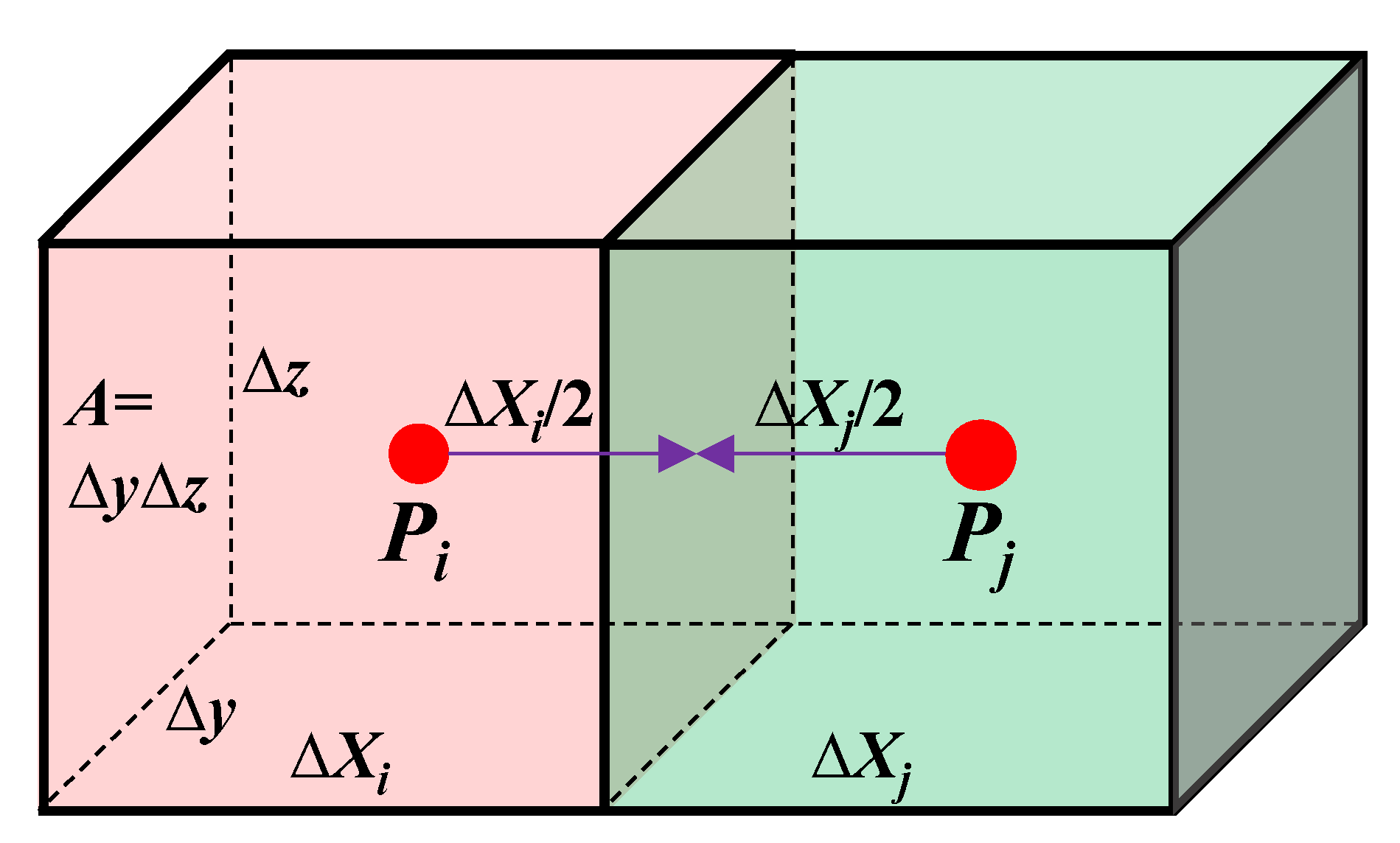
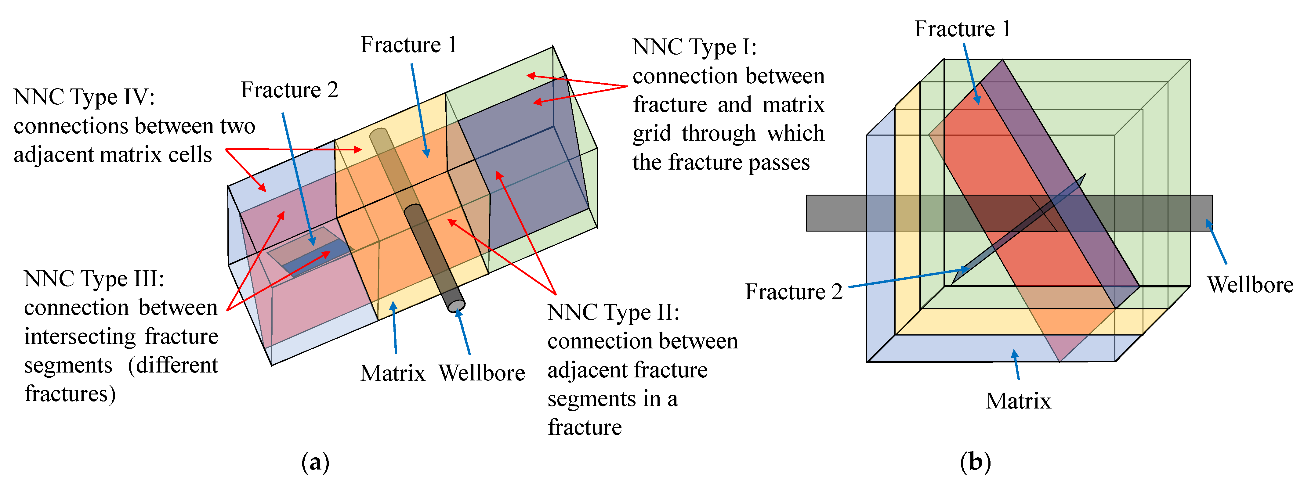
2.2. Finite Volume Discretization of Flow Equations for 3D-EDFM

For 3D-EDFM, rectangular parallelepiped grids are generally chosen to solve the geometrical parameters between the fracture surface and the matrix [33]. In this set of grid systems, the finite volume method that satisfies the local mass balance and has clear physical meaning is the preferred choice. Therefore, the finite volume method is used to discretize the flow equation for the cuboid matrix grid. The details are as follows:
We take the oil component equation as an example to illustrate the finite volume discrete scheme of flow equations. In this paper, the block-center finite volume method is adopted. The block-center control volume is the volume of gridblock where the block center is located. Integrating the time and control volume on both sides of the oil-phase equation above, and using the divergence theorem, the following is obtained:
t t + Δ t { k k r o B o μ o [ p o ( γ o D ) ] } n d s d t + q o = Δ V t t + Δ t [ t ( ϕ S o B o ) ] d t d V
The area integral in the left side of Equation (4) can be approximated by the sum of normal flow rates between adjacent gridblocks that conform to physical significance. For the integration of time on the right side of the above equation, it can be solved accurately, which is why the finite volume method has high precision. Equation (4) can be rewritten as:
j = 1 n { T i j [ ( p o i p o j ) + ( γ o i D o i γ o j D o j ) ] } + q s c n + 1 = Δ V i Δ t [ ( ϕ S o B o ) t + Δ t ( ϕ S o B o ) t ]
where n is the number of other gridblocks adjacent to this gridblock; ΔVi is the volume of the gridblock; Δt is the time interval of two adjacent time steps; and Tij is the transmissibility of adjacent gridblocks, which is the product of the mobility λij and the geometric factor Gij.
The mobility λij can be expressed as:
λ i j = k r o μ o B o
In this equation, the upstream scheme is used for the value of the physical quantity kro subject to saturation. For physical quantities μo and Bo subject to pressure, the values are in the arithmetic average scheme as:
k r o = { ( k r o ) i p o , i p o , j ( k r o ) j p o , i < p o , j
μ o = μ o , i + μ o , j 2
B o = B o , i + B o , j 2
The geometric factor Gij of mass transfer between two adjacent matrix grids is equal to half of the harmonic average of geometric factors Gi and Gj in two separate grids, as shown in Figure 1. For 3D box mesh, taking the X direction as an example, we can obtain:
G i j = ( G i 1 + G j 1 ) 1
G i = k i A 2 Δ x i
G j = k j A 2 Δ x j
Similar to the oil component equation, the block-center finite volume discrete scheme of the gas component flow equation in the matrix grid is:
j = 1 n [ G i j λ g , i j ( p o , i p o , j + p c g o , i p c g o , j ) + R s , i j G i j λ o , i j ( p o , i p o , j ) + ( γ o i D o i γ o j D o j ) ] n + 1 + q g s c n + 1 + R s , i q o s c n + 1 = Δ V i Δ t [ ( ϕ S g , i B g ) n + 1 ( ϕ S g , i B g ) n + ( R s ϕ ( 1 S g , i S w , i ) B o ) t + Δ t ( R s ϕ ( 1 S g , i S w , i ) B o ) t ]
In this paper, for flow between fracture units, the block-center finite volume method is still used to discretize the flow equation. Taking the oil component equation as an example, the discrete scheme can be obtained as follows:
j = 1 n { T f i j [ ( p o f i p o f j ) + ( γ o f i D o f i γ o f j D o f j ) ] } + q o m f = Δ V i Δ t [ ( ϕ f S o f , i B o ) t + Δ t ( ϕ f S o f , i B o ) t ]
where n is the number of fracture units adjacent to the ith fracture unit; Tfij is the transmissibility of the ith and jth fracture units; pofi, pofj are the oil-phase pressure at the center of ith and jth fracture units; γofi, γofj are the oil-phase gravity at the center of ith and jth fracture units; Dofi, Dofj are the depths at which the centers of ith and jth fracture units are located (negative number); qomf is the transfer flux term of the matrix grid to the fracture unit; ΔVi is the volume of the ith fracture unit; Δt is the time increment; φf, Soj,i are the porosity and saturation of the ith fracture unit; and Bo is the oil-phase volume factor corresponding to the ith fracture unit.
It can be seen from Equations (5) and (13) that the key to determining the specific discrete scheme of the flow equation of fracture units is to determine the transmissibility Tfij of fracture units, and the calculation of the geometric factor Gfij in the transmissibility is related to the connection relationship between fracture units. As shown in Figure 2, after dividing the fracture by matrix grid boundary, four types of Non-Neighboring Connection (NNC) in 3D-EDFM are formed, which are the connection between the fracture segment and the matrix grid through which the fracture section passes (NNC Type I), the connection between adjacent fracture segments in a fracture (NNC Type II), the connection between intersecting fracture segments (different fractures, NNC Type III), and the connection between two adjacent matrix cells (NNC Type IV). Introducing NNC pairs enables flow exchange between grids that are not only adjacent in the physical model but also adjacent in the computational model. The general calculation equation of the transmissibility coefficient of NNC is:
T N N C = K N N C A N N C d N N C
where KNNC is the permeability of NNC, i.e., the effective permeability, mD; ANNC is the contact area of NNC, i.e., the open area, m2; and dNNC is the characteristic distance associated with NNC, m.

2.3. Characterization of CO2 Physical Properties Change
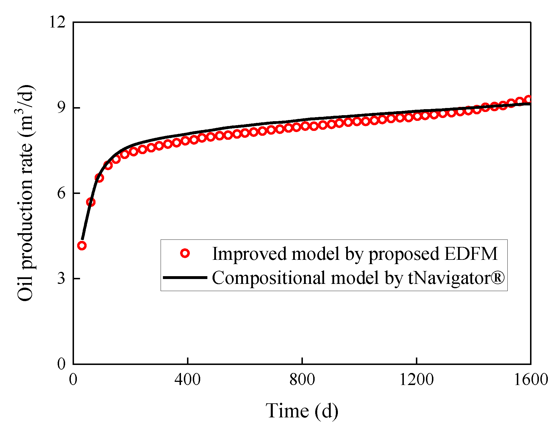
Ordos Basin may be the most favorable and suitable place for CCUS in China. This paper studies the Chang-7 reservoir of Changqing Oilfield, which is located in the south of Ordos Basin, as shown in Figure 3. Due to the low reservoir pressure, it is difficult for oil and gas to reach the miscible state after CO2 injection, and the component change is not violent. Therefore, gas injection into oil reservoirs can be simplified as a two-phase two-component problem, which can be treated by the black oil model.
To evaluate the effect of injected gas, it is necessary to accurately calculate the PVT properties of CO2. The main oil recovery mechanism of CO2 immiscible flooding is to reduce the viscosity of crude oil, expand the volume of crude oil, extract and vaporize light hydrocarbons in crude oil, and reduce interfacial tension. This kind of CO2-EOR is usually characterized by the changing of CO2 physical properties. According to the D-A-K method introduced by Dranchuk et al. [35], the properties of CO2 under different reservoir pressures can be obtained as shown in Equation (16).
B g = V V s c = Z T P s c T s c P = Z 273 + t 273 P s c P
The Lee–Gonzalez–Eakin equations [36], such as Equations (17) and (18), are used for a semi-empirical method to calculate gas viscosity as:
μ g = 10 4 K exp ( X ρ g Y )
K = 10 4 exp ( X ρ g Y ) 209.2 + 19.26 M g + 1.8 T
It is well known that the molecular weight of CO2 is 44. According to the above method, the PVT properties of CO2 are calculated iteratively, and the results are shown in Table 1. With the increase in reservoir pressure, the volume coefficient of CO2 gradually decreases, but the viscosity of CO2 increases. The effect of CO2 injection can be approximated by introducing the pressure-dependent physical properties of CO2 into the black oil model.

3. Model Validation

In our previous research [37], the accuracy of the proposed embedded discrete fracture modeling has been verified. Combined with the varying pressure-related fluid physical properties, the accuracy of the improved black oil model in this paper is compared with the compositional model from the advanced reservoir simulation software named tNavigator® for evaluating the injection of CO2. The values of parameters used in the simulation are shown in Table 2. Based on the physical scenario of one-well injection and one-well production (as shown in Figure 4), the reservoir pressure distribution of the improved model by our EDFM is consistent with that of the compositional model by tNavigator®, as indicated in Figure 5. Similarly, the results of well production performance between the two simulators are remarkably similar, as illustrated in Figure 6. The above verification shows that the model proposed in this paper can reflect dynamic characteristics affected by injecting CO2.

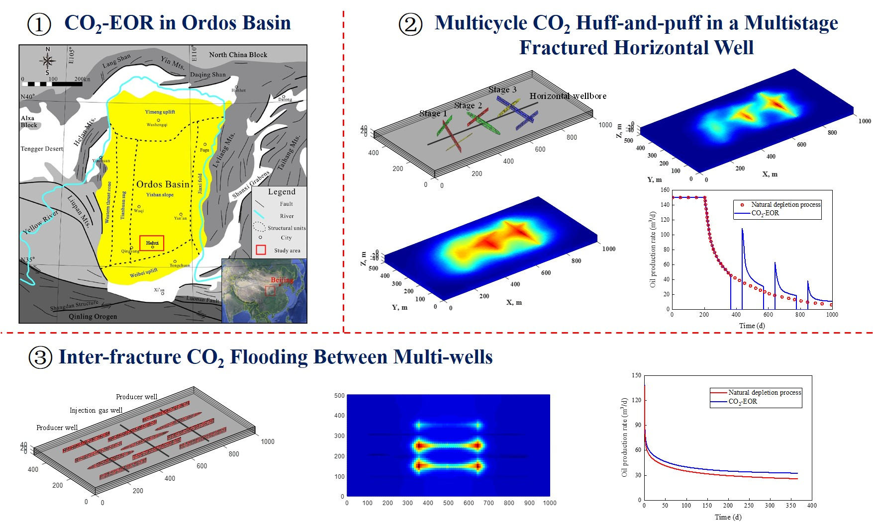
4. Application Cases

In this section, two numerical examples of single-well multicycle CO2 huff-and-puff and multi-well inter-fracture CO2 flooding are introduced to demonstrate the engineering application of the proposed model in CO2-EOR and carbon sequestration. Both examples are aimed at the Chang-7 reservoir in Ordos Basin, and basic parameters are consistent. Table 3 summarizes the model physical properties of the reservoir and fluids, such as rock, fracture, injection gas (CO2), and crude oil. As shown in Figure 7, there are relative permeability and capillary pressure curves in matrix, which reflects the flowability of oil and gas in reservoirs.

4.1. Multicycle CO2 Huff-and-Puff in a Multistage Fractured Horizontal Well

In this example, 3D-EDFM is applied for the production simulation of multicycle CO2 huff-and-puff in a multistage fractured horizontal well. Figure 8 shows the front view, overhead view, and 3D view of the reservoir model for a three-stage fractured horizontal well. The biggest difference between 3D-EDFM and 2D-EDFM is that the 3D model can capture the characteristics of arbitrary-placed inclined fractures with arbitrary shapes. It can be seen that our simulator can efficiently calibrate the hydraulic fracture networks using given information and characterize more complex spatial positions and fracture shapes, which is hardly achieved by commercial software such as tNavigator® that only can handle situations in which fractures are aligned with axes.
The fractured horizontal well of this model is controlled at a fixed oil production of 150 m3/d. When the reservoir pressure is lower than the economic limit pressure, the production well will be transformed into a CO2 huff-and-puff huff working system. The cycle of CO2 huff-and-puff is 135 days, and the interval between cycles is 70 days. The injection pressure of CO2 is set at a fixed 30 MPa. Figure 9 shows the production dynamic curves of multicycle CO2 huff-and-puff with varying matrix permeability. It can be concluded that multicycle CO2 injection can indeed improve oil recovery in low-permeability reservoirs, which is significantly related to the matrix permeability. The higher the matrix permeability, the greater the degree of CO2-EOR. It shows, as another aspect, that hydraulic fracturing is an important prerequisite for CO2-EOR in low-permeability unconventional reservoirs. Figure 10 shows the CO2 saturation distribution map at different stages of multicycle CO2 huff-and-puff. The free CO2 accumulates near the fracture networks and gradually flows from the fracture to the matrix.

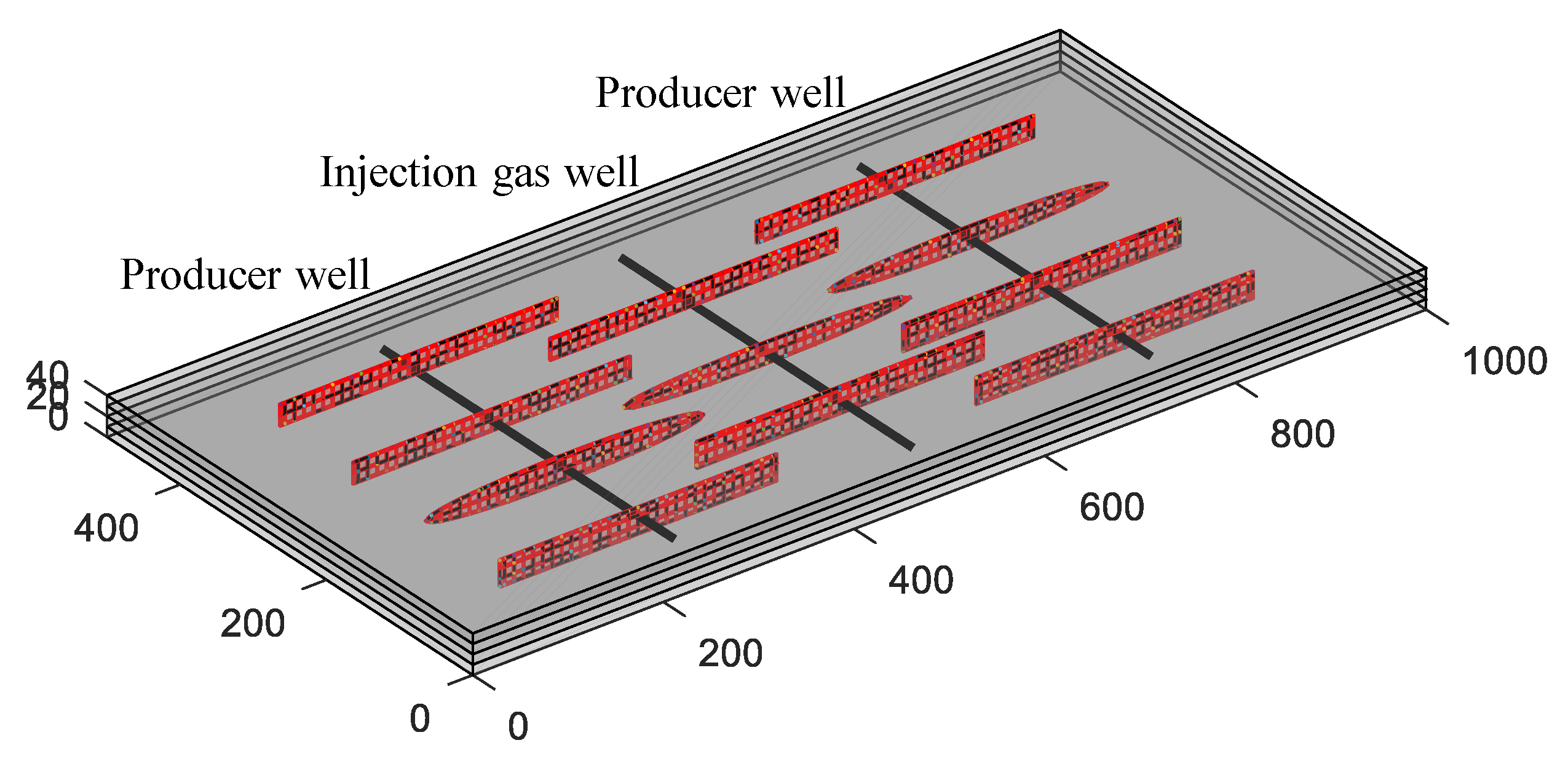
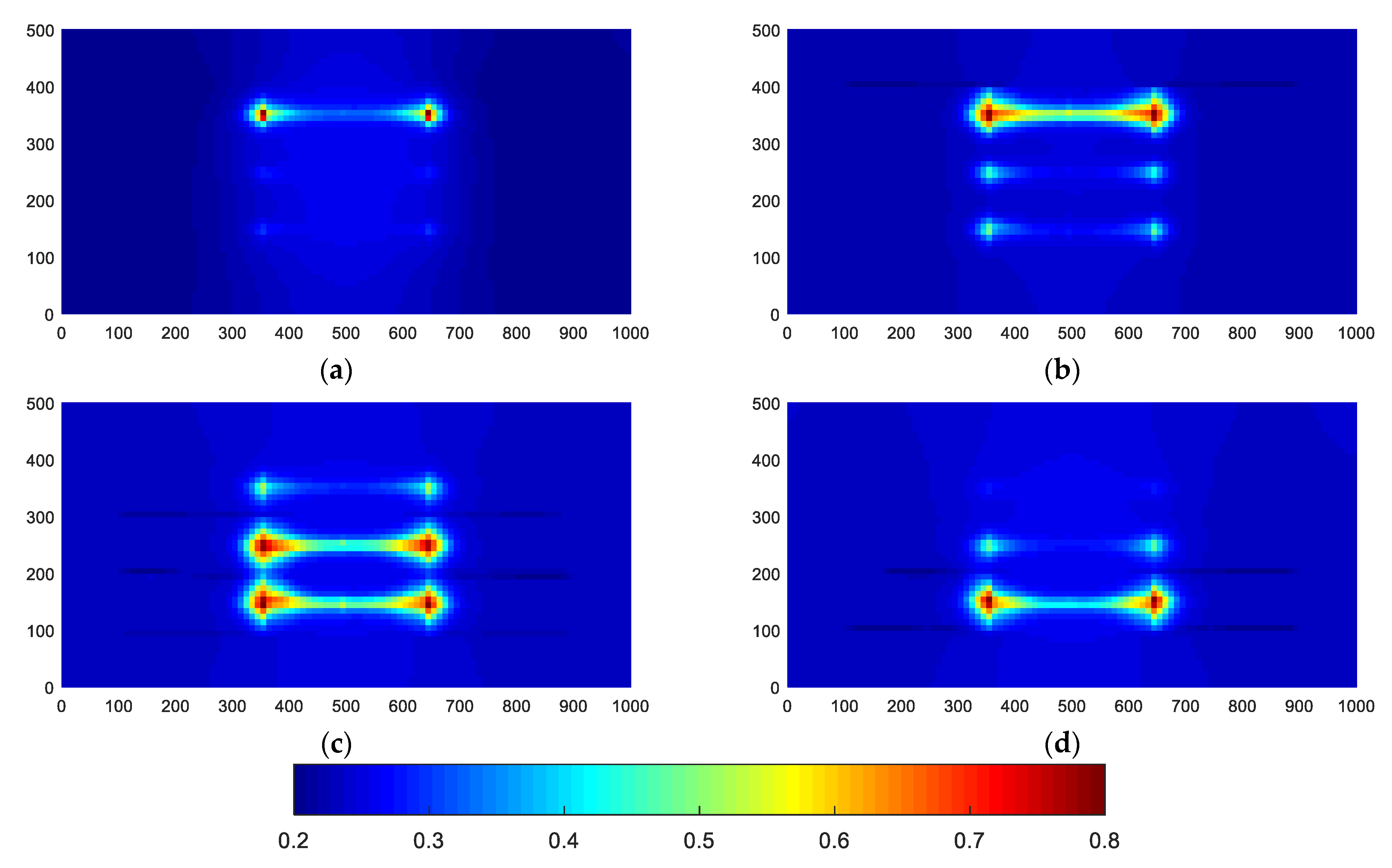
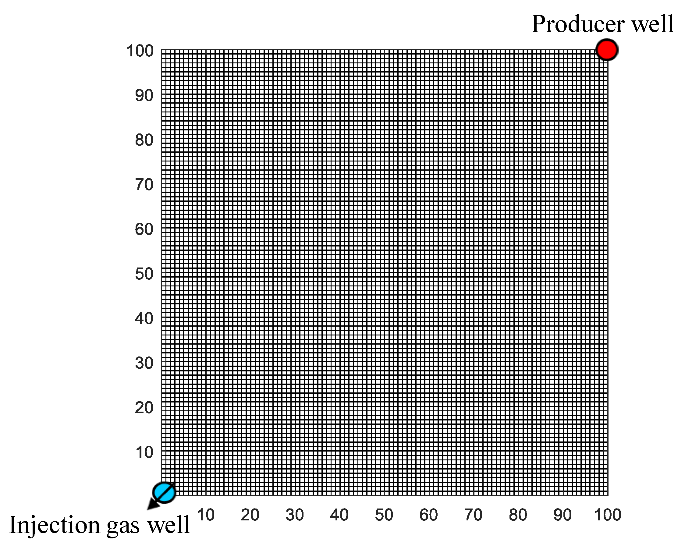
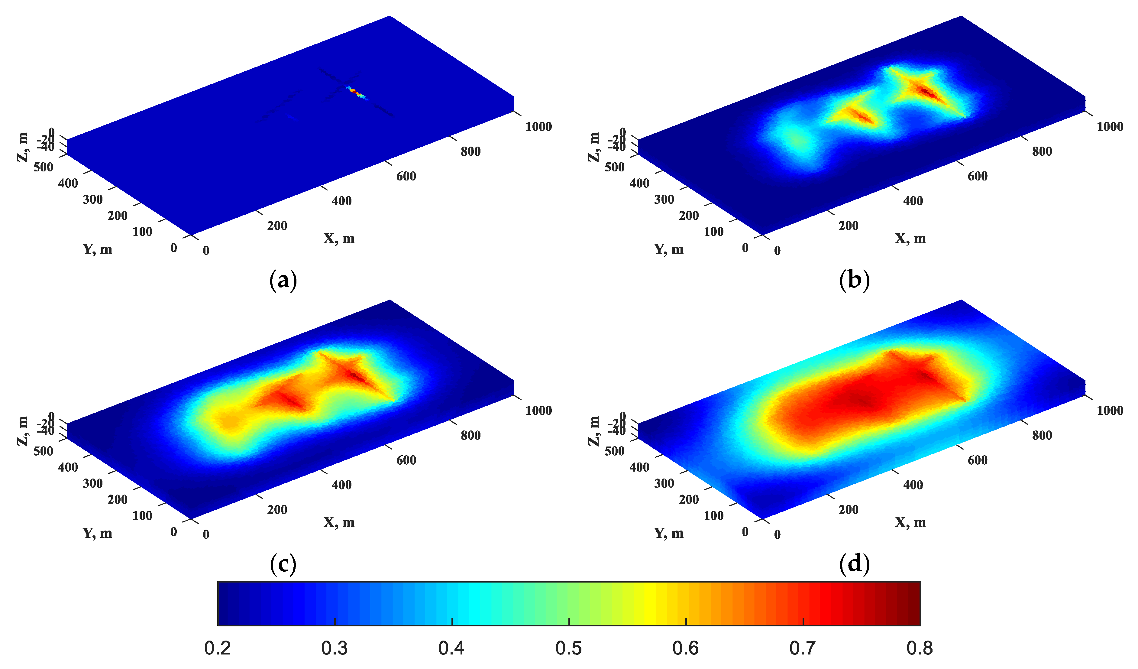
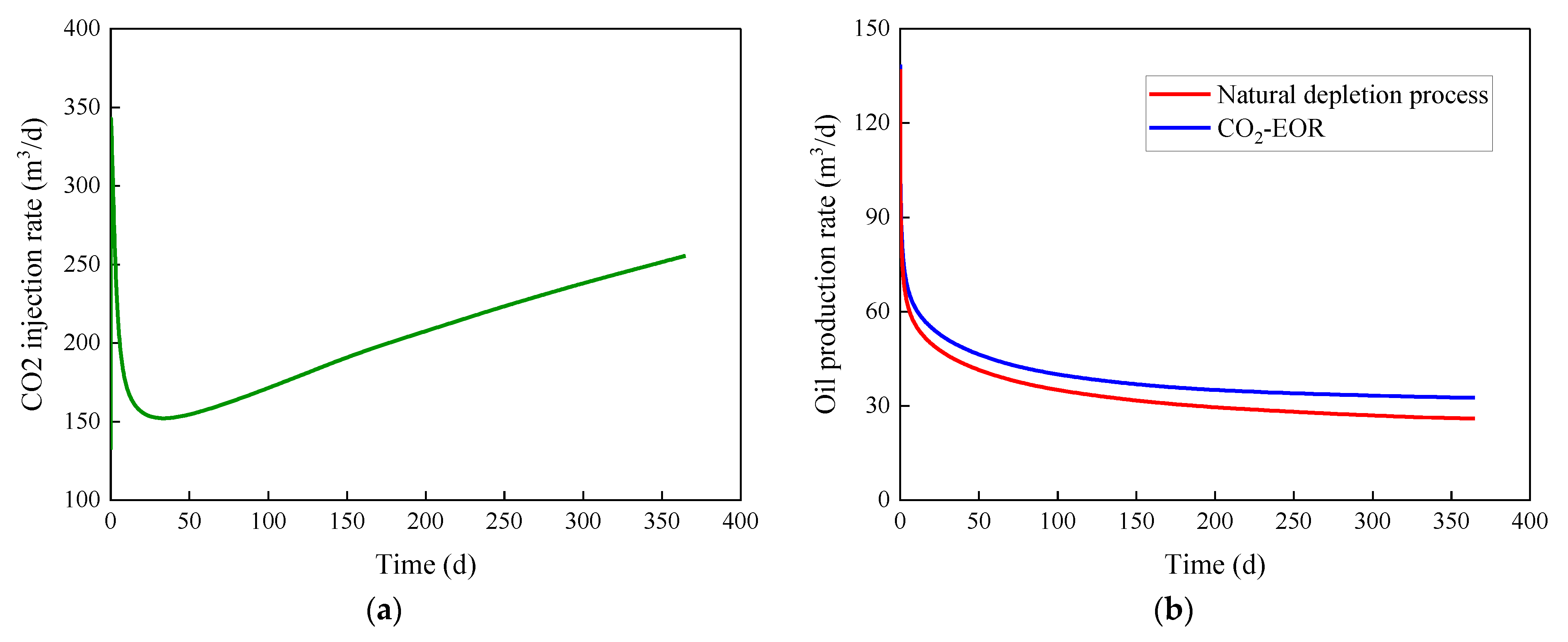
4.2. Inter-Fracture CO2 Flooding between Multi-Wells

In this case, 3D-EDFM is applied for simulating the inter-fracture CO2 flooding between multiple wells. Figure 11 shows the sketch of three horizontal wells, of which one injection well is located in the middle of two production wells. The oil production and gas injection are carried out simultaneously. The bottom hole pressure is constantly controlled at 10 MPa and 30 MPa when it is producing and injecting, respectively. Figure 12 summarizes the plot of production dynamic curves of simulation of 1 year, and Figure 12a shows the dynamic change of gas injection rate. Figure 12b illustrates that the daily oil production considered CO2 flooding is higher than that of the natural depletion process without the effect of CO2 injection. In this model, the first fracture of the injection gas well is located in the first and second layers, and the second and third fractures are located in the third and fourth layers. The proposed 3D-EDFM can also be used to model the location of fractures in different layers, which is more consistent with the actual formation and engineering conditions. Figure 13 shows the CO2 saturation distribution map of simulation of 1 year at different layers. It can be seen that the injected CO2 will preferentially diffuse along the fracture and the diffusion area is not large enough because the simulated production time is relatively short. The effect of CO2 geological sequestration can be assessed by prolonging the production time because it is a long-term process. The extra significance of this model is that the asynchronous injection and production process can be stimulated by further controlling the open–shut time of wells, which is also worthy of attention in engineering applications.

5. Conclusions

This paper presents a CO2-EOR evaluation model based on 3D-EDFM. The model can effectively describe the three-dimensional fractured geological conditions of low-permeability reservoirs, which cannot be effectively handled by general business software. Practical applications of this model in simulating the CO2 huff-and-puff in single-well and inter-fracture CO2 flooding between multi-wells are illustrated. The results of simulations show that the proposed model can handle the complex shapes of fractures and arbitrary spatial positions distribution in 3D reservoirs and can be adopted to evaluate CO2-EOR and geological sequestration problems. This paper is a preliminary theoretical attempt to discuss the modeling techniques for green energy transition, and we will explore more possibilities for this model in the future.

Author Contributions

Conceptualization, X.D.; Investigation, J.Z.; Methodology, X.D.; Software, X.D.; Supervision, L.C. and R.C.; Validation, J.Z.; Visualization, J.Z.; Writing—original draft, X.D. All authors have read and agreed to the published version of the manuscript.

Funding

This work was funded by National Natural Science Foundation of China (No. U1762210, No. 51674273, and No. 52174038), National Science and Technology Major Project of China (No. 2017ZX05069-003), and China Petroleum Science and Technology Program (Major Program, Grant No. ZLZX2020-02-04).

Institutional Review Board Statement

Not applicable.

Informed Consent Statement

Not applicable.

Data Availability Statement

Not applicable.

Acknowledgments

Xulin Du expresses gratitude to Xiang Rao at Yangtze University for his valuable suggestions and discussions on this work.

Conflicts of Interest

The authors declare no conflict of interest.

References

  1. Zhou, Y.B.; Chen, X.; Tan, X.; Liu, C.Y.; Zhang, S.N. Mechanism of CO2 Emission Reduction by Global Energy Interconnection. Glob. Energy Interconnect. 2018, 1, 11–21. [Google Scholar]
  2. Zhang, X.; Geng, Y.; Shao, S.; Dong, H.J.; Wu, R.; Yao, T.L.; Song, J.K. How to Achieve China’s CO2 Emission Reduction Targets by Provincial Efforts?—An Analysis Based on Generalized Divisia Index and Dynamic Scenario Simulation. Renew. Sustain. Energy Rev. 2020, 127, 109892. [Google Scholar] [CrossRef]
  3. Paul, B.; Extavour, M. CCUS: Utilizing CO2 to Reduce Emissions. Chem. Eng. Prog. 2016, 6, 52–59. [Google Scholar]
  4. Yan, Y.L.; Borhani, T.N.; Subraveti, S.G.; Pai, K.N.; Prasad, V.; Rajendran, A.; Nkulikiyinka, P.; Asibor, J.O.; Zhang, Z.E.; Shao, D.; et al. Harnessing the Power of Machine Learning for Carbon Capture, Utilisation, and Storage (CCUS)—A State-of-the-art Review. Energy Environ. Sci. 2021, 14, 6122–6157. [Google Scholar] [CrossRef]
  5. Hasan, M.M.F.; First, E.L.; Boukouvala, F.; Floudas, C.A. A Multi-scale Framework for CO2 Capture, Utilization, and Sequestration: CCUS and CCU. Comput. Chem. Eng. 2015, 81, 2–21. [Google Scholar] [CrossRef] [Green Version]
  6. Ji, L.; Yu, H.; Li, K.K.; Yu, B.; Grigore, M.; Yang, Q.; Wang, X.L.; Chen, Z.L.; Zeng, M.; Zhao, S.F. Integrated Absorption-mineralisation for Low-energy CO2 Capture and Sequestration. Appl. Energy 2018, 225, 356–366. [Google Scholar] [CrossRef]
  7. Akindipe, D.; Saraji, S.; Piri, M. Salt Precipitation during Geological Sequestration of Supercritical CO2 in Saline Aquifers: A Pore-scale Experimental Investigation. Adv. Water Resour. 2021, 155, 104011. [Google Scholar] [CrossRef]
  8. Harris, J.; Kovscek, A. Geological Storage of Carbon Dioxide Technical Report Global Climate and Energy Project (GCEP); Stanford University: Stanford, CA, USA, 2009. [Google Scholar]
  9. Hajiabadi, S.H.; Bedrikovetsky, P.; Borazjani, S.; Mahani, H. Well Injectivity during CO2 Geosequestration: A Review of Hydro-Physical, Chemical and Geomechanical Effects. Energy Fuels 2021, 35, 9240–9267. [Google Scholar] [CrossRef]
  10. Bachu, S. Identification of Oil Reservoirs Suitable for CO2-EOR and CO2 Storage (CCUS) Using Reserves Databases, with Application to Alberta, Canada. Int. J. Greenh. Gas Control. 2016, 44, 152–165. [Google Scholar] [CrossRef]
  11. Welkenhuysen, K.; Rupert, J.; Compernolle, T.; Ramirez, A.; Swennen, R.; Piessens, K. Considering Economic and Geological Uncertainty in the Simulation of Realistic Investment Decisions for CO2-EOR Projects in the North Sea. Appl. Energy 2017, 185, 745–761. [Google Scholar] [CrossRef]
  12. Cai, M.Y.; Su, Y.L.; Elsworth, D.; Li, L.; Fan, L.Y. Hydro-mechanical-chemical Modeling of Sub-nanopore Capillary-confinement on CO2-CCUS-EOR. Energy 2021, 225, 120203. [Google Scholar] [CrossRef]
  13. Zhao, J.Y.; An, X.P.; Wang, J.; Fan, J.M.; Kang, X.M.; Tian, X.Q.; Li, W.Q. A Quantitative Evaluation for Well Pattern Adaptability in Ultra-low Permeability Oil Reservoirs: A Case Study of Triassic Chang 6 and Chang 8 Reservoirs in Ordos Basin. Petrol. Explor. Dev. 2018, 45, 125–132. [Google Scholar] [CrossRef]
  14. Wang, Y.; Hou, J.R.; Song, Z.J.; Yuan, D.Y.; Zhang, J.W.; Zhao, T. Simulation Study of In-Situ CO2 Huff-n-Puff in Low Permeability Fault-Block Reservoirs. In Proceedings of the 2015 SPE Asia Pacific Oil & Gas Conference & Exhibition, Nusa Dua, Bali, Indonesia, 20–22 October 2015; p. 176327. [Google Scholar]
  15. Yang, Z.G.; Yue, X.G.; Shao, M.L.; Yang, Y.; Yan, R.J. Monitoring of Flooding Characteristics with Different Methane Gas Injection Methods in Low-Permeability Heterogeneous Cores. Energy Fuels 2021, 35, 3208–3218. [Google Scholar] [CrossRef]
  16. Shen, H.; Yang, Z.H.; Li, X.C.; Peng, Y.; Lin, M.Q.; Zhang, J.; Dong, Z.X. CO2-responsive Agent for Restraining Gas Channeling during CO2 Flooding in Low Permeability Reservoirs. Fuel 2021, 292, 120306. [Google Scholar] [CrossRef]
  17. Cao, R.Y.; Xu, X.Z.; Cheng, L.S.; Peng, Y.Y.; Wang, Y.; Guo, Z.L. Study of Single Phase Mass Transfer between Matrix and Fracture in Tight Oil Reservoirs. Geofluids 2019, 2019, 1038412. [Google Scholar] [CrossRef]
  18. Jia, P.; Cheng, L.S.; Huang, S.J.; Liu, H.J. Transient Behavior of Complex Fracture Networks. J. Pet. Sci. Eng. 2015, 132, 1–17. [Google Scholar] [CrossRef]
  19. Warren, J.; Root, P. The behavior of Naturally Fractured Reservoirs. SPE J. 1963, 3, 245–255. [Google Scholar] [CrossRef] [Green Version]
  20. Kazemi, H.; Seth, M.S.; Thomas, G.W. The Interpretation of Interference Tests in Naturally Fractured Reservoirs with Uniform Fracture Distribution. SPE J. 1969, 9, 463–472. [Google Scholar]
  21. Swann, A.D. Analytical Solution for Determining Naturally Fractured Reservoir Properties by Well Testing. SPE J. 1976, 16, 117–122. [Google Scholar]
  22. Al-Ahmadi, H.A.; Wattenbarger, R.A. Triple-porosity Models: One Further Step towards Capturing Fractured Reservoirs Heterogeneity. In Proceedings of the 2011 SPE/DGS Saudi Arabia Section Technical Symposium and Exhibition, Al-Khobar, Saudi Arabia, 15–18 May 2011; p. 149054. [Google Scholar]
  23. Al-Ahmadi, H.A. A Triple-Porosity Model for Fractured Horizontal Wells. Ph.D. Thesis, Texas A&M University, College Station, TX, USA, 2010. [Google Scholar]
  24. Jones, J.R.; Volz, R.; Diasmari, W. Fracture Complexity Impacts on Pressure Transient Responses from Horizontal Wells Completed with Multiple Hydraulic Fracture Stages. In Proceedings of the 2013 SPE Unconventional Resources Conference Canada, Calgary, AB, Canada, 5–7 November 2013; p. 167120. [Google Scholar]
  25. Cipolla, C.L. Modeling Production and Evaluating Fracture Performance in Unconventional Gas Reservoirs. J. Pet. Technol. 2009, 61, 84–90. [Google Scholar] [CrossRef]
  26. Cipolla, C.L.; Williams, M.J.; Weng, X.W.; Mack, M.G.; Maxwell, S.C. Hydraulic Fracture Monitoring to Reservoir Simulation: Maximizing Value. In Proceedings of the 2010 SPE Annual Technical Conference and Exhibition, Florence, Italy, 19–22 September 2010; p. 133877. [Google Scholar]
  27. Lee, S.H.; Jensen, C.L.; Lough, M.F. Efficient Finite-Difference Model for Flow in a Reservoir with Multiple Length-Scale Fractures. SPE J. 2000, 5, 268–275. [Google Scholar] [CrossRef]
  28. Moinfar, A.; Varavei, A.; Sepehrnoori, K.; Johns, R. Development of an Efficient Embedded Discrete Fracture Model for 3D Compositional Reservoir Simulation in Fractured Reservoirs. SPE J. 2014, 19, 289–303. [Google Scholar] [CrossRef] [Green Version]
  29. Moinfar, A.; Sepehrnoori, K.; Johns, R.T.; Varavei, A. Coupled Geomechanics and Flow Simulation for An Embedded Discrete Fracture Model. In Proceedings of the 2013 SPE Reservoir Simulation Symposium, Woodlands, TX, USA, 18–20 February 2013; p. 163666. [Google Scholar]
  30. Tene, M.; Bosma, S.B.M.; Al Kobaisi, M.S.; Hajibeygi, H. Projection-based Embedded Discrete Fracture Model (pEDFM). Adv. Water Resour. 2017, 105, 205–216. [Google Scholar] [CrossRef]
  31. Rao, X.; Cheng, L.S.; Cao, R.Y.; Jia, P.; Liu, H.; Du, X.L. A Modified Projection-based Embedded Discrete Fracture Model (pEDFM) for Practical and Accurate Numerical Simulation of Fractured Reservoir. J. Petrol. Sci. Eng. 2020, 187, 106852. [Google Scholar] [CrossRef]
  32. Cao, R.Y.; Fang, S.D.; Jia, P.; Cheng, L.S.; Rao, X. An Efficient Embedded Discrete-fracture Model for 2D Anisotropic Reservoir Simulation. J. Petrol. Sci. Eng. 2019, 174, 115–130. [Google Scholar] [CrossRef]
  33. Rao, X.; Cheng, L.S.; Cao, R.Y.; Jia, P.; Wu, Y.H.; He, Y.M.; Chen, Y. An Efficient Three-dimensional Embedded Discrete Fracture Model for Production Simulation of Multi-stage Fractured Horizontal Well. Eng. Anal. Bound. Elem. 2019, 106, 473–492. [Google Scholar] [CrossRef]
  34. Chen, Y.H.; Wang, Y.B.; Guo, M.Q.; Wu, H.Y.; Li, J.; Wu, W.T.; Zhao, J.Z. Differential Enrichment Mechanism of Organic Matters in the Marine-continental Transitional Shale in Northeastern Ordos Basin, China: Control of Sedimentary Environments. J. Nat. Gas. Sci. Eng. 2020, 83, 103625. [Google Scholar] [CrossRef]
  35. Dranchuk, P.M.; Kassem, H. Calculation of Z Factors for Natural Gases Using Equations of State. J. Can. Petrol. Technol. 1975, 14, 86–91. [Google Scholar] [CrossRef]
  36. Lee, A.L.; Gonzalez, M.H.; Eakin, B.E. The Viscosity of Natural Gases. J. Pet. Technol. 1966, 18, 997–1000. [Google Scholar] [CrossRef]
  37. Du, X.L.; Cheng, L.S.; Chen, J.; Cai, J.C.; Niu, L.Y.; Cao, R.Y. Numerical Investigation for Three-Dimensional Multiscale Fracture Networks Based on a Coupled Hybrid Model. Energies 2021, 14, 6354. [Google Scholar] [CrossRef]
Figure 1. Sketch of discretization for rectangular matrix gridblocks.
Atmosphere 13 00229 g001
Figure 2. The NNCs of three-dimensional embedded discrete fracture model. (a) Front side view of the model. (b) Left side view of the model.
Atmosphere 13 00229 g002
Figure 3. Regional geological map of Ordos Basin and study area (modified after Chen et al. [34]).
Atmosphere 13 00229 g003
Figure 4. The physical scenario of one-well injection and one-well production.
Atmosphere 13 00229 g004
Figure 5. Comparison of pressure distribution maps between two simulators. (a) Compositional model by tNavigator®. (b) Improved model by proposed EDFM.
Atmosphere 13 00229 g005
Figure 6. Comparison of well production performance between two simulators.
Atmosphere 13 00229 g006
Figure 7. The relative permeability and capillary pressure curves in matrix. (a) The relative permeability curves. (b) The capillary pressure curve.
Atmosphere 13 00229 g007
Figure 8. Sketch of 3D reservoir model with fracture cells and the horizontal wellbore. (a) 3D view. (b) Top view. (c) Main view.
Atmosphere 13 00229 g008
Figure 9. Production dynamic curves of multicycle CO2 huff-and-puff with varying matrix permeability. (a) Matrix permeability 10 mD. (b) Matrix permeability 1 mD. (c) Matrix permeability 0.5 mD. (d) Matrix permeability 0.1 mD.
Atmosphere 13 00229 g009
Figure 10. The CO2 saturation distribution map at different stages of multicycle CO2 huff-and-puff. (a) The start time. (b) After the 1st cycle. (c) After the 2nd cycle. (d) After the 3rd cycle.
Atmosphere 13 00229 g010
Figure 11. Sketch of inter-fracture CO2 flooding between multiple wells.
Atmosphere 13 00229 g011
Figure 12. Production dynamic curves of inter-fracture CO2 flooding between multi-wells. (a) CO2 injection rate under constant pressure. (b) Oil production rate under constant pressure.
Atmosphere 13 00229 g012
Figure 13. The CO2 saturation distribution map of simulation of 1 year at different layers. (a) The 1st layer. (b) The 2nd layer. (c) The 3rd layer. (d) The 4th layer.
Atmosphere 13 00229 g013
Table 1. The PVT property of CO2.
Reservoir Pressure, MPaThe Volume Coefficient of CO2, m3/m3The Viscosity of CO2, mPa·s
3.450.0300.012
6.900.0120.016
10.340.0070.026
15.170.0050.041
17.930.0050.047
20.690.0050.052
23.450.0040.057
25.520.0040.061
27.030.0040.063
28.970.0040.066
Table 2. Parameters of the numerical simulation case.
PropertiesValuePropertiesValue
Grid size, m1 × 1 × 10Initial reservoir pressure, MPa14.1
Number of grids100 × 100 × 1CO2 density (SC), g/L1.96
Initial oil saturation, fraction0.8Initial gas–oil ratio, m3/m368.17
Reservoir depth, m1600Oil density (SC), kg/m3820
Layer thickness, m10Rock compressibility, MPa −11.07 × 10⁻⁴
Injection pressure, MPa25Production pressure, MPa10
Table 3. Physical properties of the reservoir and fluids.
PropertiesValuePropertiesValue
Reservoir volume, m1000 × 500 × 30Grid number100 × 50 × 3
Reservoir depth, m1500Initial reservoir pressure, MPa30
Well diameter, m0.178Skin factor, fraction0.1
Rock compressibility, MPa−11.07 × 10⁻⁴Fracture aperture, m0.01
Matrix porosity, fraction0.17Fracture porosity, fraction0.4
Matrix permeability, mD1Fracture permeability, mD20,000
CO2 density (SC), g/L1.96Oil density (SC), kg/m3820
Oil viscosity, mPa·s2Oil compressibility, MPa−13.02 × 10⁻³
Publisher’s Note: MDPI stays neutral with regard to jurisdictional claims in published maps and institutional affiliations.

