Article

Multi-Case Analysis of Ice Particle Properties of Stratiform Clouds Using In Situ Aircraft Observations in Hebei, China

1
College of Global Change and Earth System Science, State Key Laboratory of Earth Surface Processes and Resource Ecology, Beijing Normal University, Beijing 100875, China
2
Key Laboratory for Cloud Physics of China Meteorological Administration, Beijing 100081, China
3
Weather Modification Office of Hebei Province, Shijiazhuang 072150, China
*
Authors to whom correspondence should be addressed.
Atmosphere 2022, 13(2), 200; https://doi.org/10.3390/atmos13020200
Submission received: 14 December 2021 / Revised: 18 January 2022 / Accepted: 25 January 2022 / Published: 26 January 2022
(This article belongs to the Special Issue Feature Papers in Atmosphere Science)

Abstract

:
This study investigates the size distribution, the mean diameter, and the concentration of ice particles within stratiform clouds by using in situ observations from 29 flights in Hebei, China. Furthermore, it examines the empirical fitting of ice particle size distributions at different temperatures using Gamma and exponential functions. Without considering the first three bins of ice particles, the mean diameter of ice particles (size range 100–1550 µm) is found to increase with temperature from −15 to −9 °C but decrease with temperature from −9 to 0 °C. By considering the first three bins of ice particles using the empirical Gamma fitting relationship found in this study, the mean diameter of ice particles (size range 25–1550 µm) shows a similar variation trend with temperature, while the turning point changes from −9 to −10 °C. The ice particle number concentration increases from 13.37 to 50.23 L−1 with an average of 31.27 L−1 when temperature decreases from 0 to −9 °C. Differently, the ice concentration decreases from 50.23 to about 22.4 L−1 when temperature decreases from −9 to −12 °C. The largest mean diameter of ice particles at temperatures around −9 and −10 °C is most likely associated with the maximum difference of ice and water supersaturation at that temperature, making the ice particles grow the fastest. These findings provide valuable information for future physical parameterization development of ice crystals within stratiform clouds.

1. Introduction

Clouds play an important role in the Earth’s radiative energy balance, including ice clouds. Better understanding of ice particle properties is critical for developing parameterizations for mesoscale and climate models [1,2,3,4,5]. Particularly, the improvement in ice particle size distribution (PSD) is extremely useful for simulating ice properties in various models [6,7,8,9,10,11]. However, affected by topography and other factors, the characteristics of ice particles vary a lot among different regions [12,13,14], making it valuable for us to analyze in detail the characteristics of ice particles over different regions.
Rangno and Hobbs [15] investigated the ice particles in stratiform clouds in the Arctic and proposed possible mechanisms for the production of high ice concentrations. They found that ice splinters generated during riming could account for the relatively high concentrations of ice particles in clouds that encompass temperatures between −2.5 and −8 °C. You et al. [16] investigated the ice particles observed by limited aircraft observations in Northeast China. They found that the ice particle concentration decreased with height, with the maximum concentration appearing in the middle and lower parts of clouds. Delanoë et al. [17] analyzed the statistical properties of the normalized ice particle size distribution, and proposed new ice PSD parameterizations, while observations over the China region are not included. Heymsfield et al. [18] summarized the observation data from a wide range of locations, temperatures, and altitudes to parameterize the ice particle size distribution and other properties. Both of these studies have made significant contributions to the science community to parameterize the ice particles from a global view. Actually, these parameterizations are believed to better represent ice PSDs at global scale, owing to a better representativeness of the in situ microphysical database used to derive it. However, these studies include no or few observations from regions over China. Further knowledge about the ice particle size distribution over regions in China is highly demanded.
There are already many studies about the ice particle properties in North China [19,20,21,22,23,24,25], but most of those studies are case studies from very limited aircraft observations. Hou et al. [24] investigated airborne measurements of ice particle properties in three stratiform precipitating clouds over northern China, finding that both exponential and Gamma functions could be used to characterize the PSD parameters. They also found that the slope values of the Gamma fitting size distribution of ice particles vary within a larger range than that of exponential fitting size distribution, and a relationship existed between the dispersion and slope values. Zhu et al. [25] investigated the ice crystal habits and growth processes in two cases of stratiform clouds with embedded convection using data observed simultaneously from three aircrafts on 18 April 2009 and 1 May 2009 as part of the Beijing Cloud Experiment (BCE). The results showed that the majority of ice crystal habits found in the two cases at temperatures between 0 and −16 °C included platelike, needle column, capped column, dendrite, and irregular. A mixture of several ice crystal habits was identified in all clouds studied.
In this study, we aim to combine as many available aircraft observations as possible to investigate the ice particle size distribution from a statistical perspective. Using the data from 29 selected aircraft observations in three years in Hebei Province, China, a multi-case based statistical analysis on the ice PSD is carried out, along with the average diameter and concentration of ice particles. The same as previous studies, we investigated the empirical fitting of ice PSDs using both Gamma and exponential fitting functions. However, different from previous studies, a greater number of aircraft observations allow us to further understand the variations in ice PSD with temperature. After comparing the fitting results between using Gamma and exponential fitting functions, we further use the Gamma fitting results to investigate the ice particle mean diameter at different temperatures with a broad size range from 25 to 1550 µm.
This paper is organized as follows. The observation data and analysis methods used in this study are described in Section 2. Section 3 shows the analysis and results regarding the stratus cloud properties. Finally, Section 4 summarizes the findings of this study.

2. Data and Method

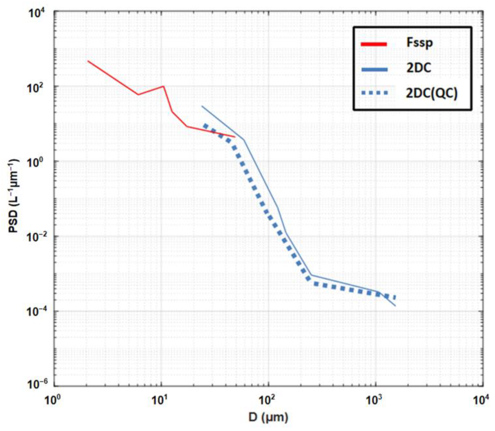
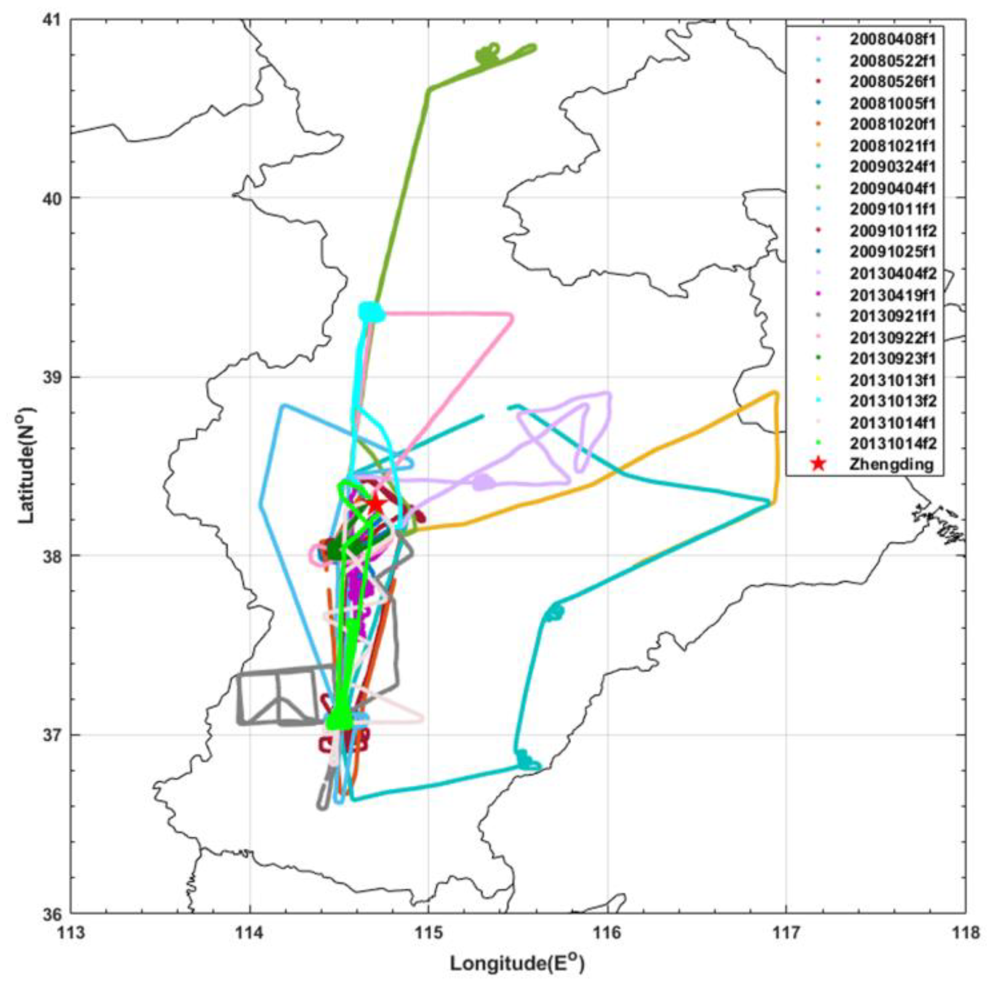
2.1. Instrument and Data

The cloud and aerosol observations from the Cheyenne aircraft, which is operated by the Hebei province Weather Modification Office, were used in this study. The instruments onboard the aircraft have been described by Zhao et al. [26] in detail. Here, we only give a brief summary description about the measurements. The Forward Scattering Spectrometer Probe Model 100 (FSSP) measures the cloud droplets with diameters from 1 to 95 μm and the two-dimensional cloud optical array probe (2DC) measures the cloud particles with a size range of 25–1550 μm (large droplets and ice crystals). The measurement ranges of the instruments onboard the aircraft are adjustable and could be different for different experiments. For example, while the detectable size range of FSSP is 1–95 µm, it has four measurement ranges to set during the experiment, which are 5–59, 2–47, 2–32, and 1–16 µm. The FSSP measurements used in this study have the size range of 2–47 µm. Note that the size range of 2DC is also adjustable and has been set up as 25–1550 µm by the field experiments used in this study. Previous studies [18,27] have explained that FSSP and 2DC data have notable limitations: (1) FSSP sizing is calibrated using spheres, with the result that non-spherical particles are undersized; (2) FSSP requires relatively high sample volumes to detect particles. By adopting the size range of 2–47 µm and considering only spherical liquid droplets, these two limitations should be minimized. In addition, noted in this study is that we only investigate the ice particle size distribution from multiple aircraft observations statistically, which can provide us with a first estimate/understanding. Further investigation about the characteristics and variation in ice particle shapes within clouds will be undertaken in the future. In order to reduce the system errors of the instruments, the first two bins of the FSSP and the first three bins of the 2DC were removed in this study by following previous studies [28,29,30,31,32].
To avoid the influence of shattering ice crystals which mainly affects small size ice crystal amount, we investigated the PSD of ice crystals observed with diameters from 100 to 1550 µm, and further examined the total ice particles within the size range of 25–100 µm based on the fitting PSD. Previous studies [18,33] used the threshold value of 200 µm to minimize the errors caused by shattering issues. Instead of 200 µm, 100 µm was used in our study due to two considerations. One is that we would like to use the direct observations from the instrument as frequently as possible rather than obtaining more from the empirical fitting regression. The other consideration is that we further confirmed the reliability of our selection of 100 µm as the threshold value via quality analysis by using the University of Illinois/Oklahoma Optical Array Probe Processing Software (UIOOPS, McFarquhar et al. [34]) to process the 2DC raw data (2DC(QC)) from limited aircraft observations (only five flights with available 2DC raw data in this study). Figure 1 shows the average spectral distribution of cloud particles with the five available in situ aircraft observations from FSSP, 2DC, and 2DC with quality checking by UIOOPS software. It is clear that the ice particle size distributions are roughly consistent between those from 2DC and 2DC(QC) for size range larger than 100 μm, with the observations from FSSP at the middle of two datasets around 100 μm. Thus, we can roughly conclude that fragmentation has little impact or a slightly overestimated impact on the particle size distribution with sizes larger than 100 μm, while it has considerable impacts for particles with sizes smaller than 100 μm. Thus, the particle observations from 2DC at the size range from 100 to 1550 µm are likely reliable in this study. Note that uncertainties for particles within the size range of 25–100 µm could be introduced by using the fitting PSD instead of observations, which is worthy of future investigation.

2.2. Method

According to previous studies, there are different methods used to identify whether the aircraft enters the cloud [35,36,37,38,39,40]. In this study, we used the method proposed by Claffey [35] and Cober [36]: when T < 0 °C, the ice particle number concentration (N) > 10 L1, and IWC > 0.001 g/m3, it is considered that the aircraft enters the ice cloud, noting that the clouds studied here are stratiform clouds which could contain both liquid and ice particles. The existence of clouds with supercooled liquid droplets was further identified based on the FSSP cloud particle number concentration (FSSP-N) and FSSP liquid water content (FSSP-LWC). When T < 0 °C, FSSP-N > 10 cm−3, and LWC > 0.001 g/m3, it is considered that supercooled water is abundant [41,42].
Based on the 2DC observations, N is calculated by integrating the ice number concentration in each size bin with ice particle diameters from 100 to 1550 µm. The ice particle mean diameter (dm) is calculated as:
dm = ΣNiDiNi
where Ni (L1) is the ice particle number concentration in the ith size bin, Di (µm) is the ice particle mean diameter in the ith size bin. There are totally 59 size bins between 100 and 1550 µm.
Table 1 shows the detailed information including flight number (named with year, month, day, and flight serial), season, flight time, ground temperature, maximum flight heights, cloud types, and total number of PSDs during each flight for the 29 in situ aircraft observations in Hebei, China, which were used in this study. Data is available from the webpage https://pan.bnu.edu.cn/l/BF2gYn (last access: 13 December 2021). The measurement time include the years 2008, 2009, and 2013, with 12 flights in spring and 17 flights in fall. Millions of samples were obtained for the ice particle size distributions during these 29 flight measurements. Figure 2 further shows the flight tracks of 20 flights, with the other nine missing due to the measurement issues in GPS. Note that all flights took off from Zhengding Airport, marked as a red star in Figure 2. It is clear that all of these observations were carried out over similar locations in south Hebei province.
According to the summary of empirical cloud PSD formula from Liu et al. [43] and other studies [44,45,46,47,48,49,50], the typical empirical PSDs include Normal, Lognormal, Exponential, Gamma (Modified Gamma), Weibull, Power-law, and multi-modal. Compared to other particle size distribution formats, Gamma distribution has been widely used by previous studies [51,52,53,54,55,56,57,58,59,60], partly because it considers the maximum entropy principle for the cloud droplet system [51] and the power-law dimensional relationships describing atmospheric particles.
We next investigated the ice PSDs using empirical fitting methods with both Gamma distribution function and exponential distribution function using the least square method. Note that Gamma distribution function could provide more accurate fitting results than the exponential distribution function as indicated by previous studies, while requiring one more parameter. In contrast, with only two parameters, the empirical fitting with exponential function could be more easily applied. The ice particle size distribution in Gamma form is:
n(D) = N0Dµ exp(−λD)
where n(D) is the ice particle number distribution at particle size D with unit of number per volume per unit size interval (L−1μm−1); N0, μ, and λ represent the three parameters of Gamma fitting function. The ice particle size distribution in exponential distribution form is:
n(D) = N0 exp(−λD)
where N0 and λ represent the two parameters of exponential fitting function. Note that in exponential PSD function, the two parameters have clear physical meanings: N0 represents the total particle number concentration and λ is related to the spectrum type [61].

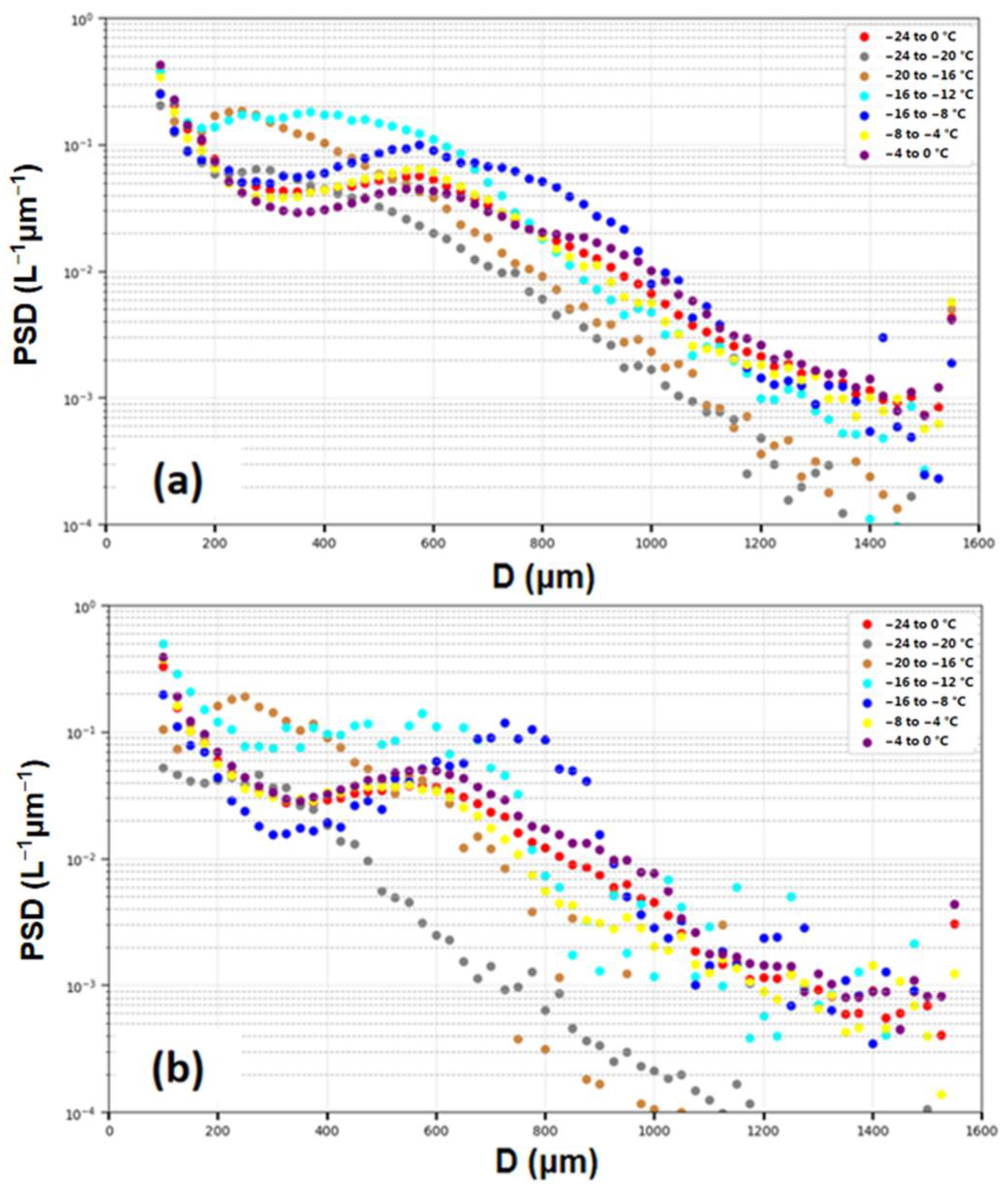
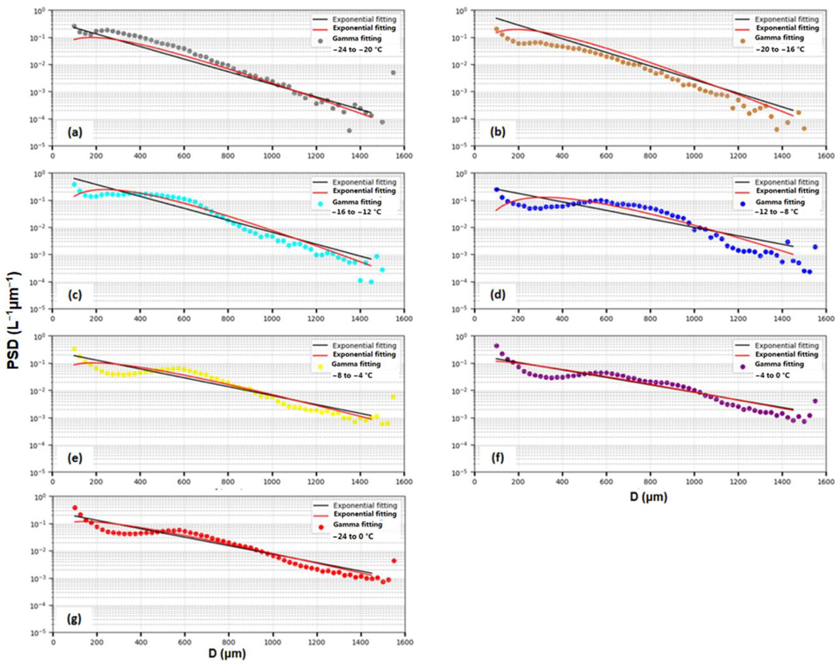
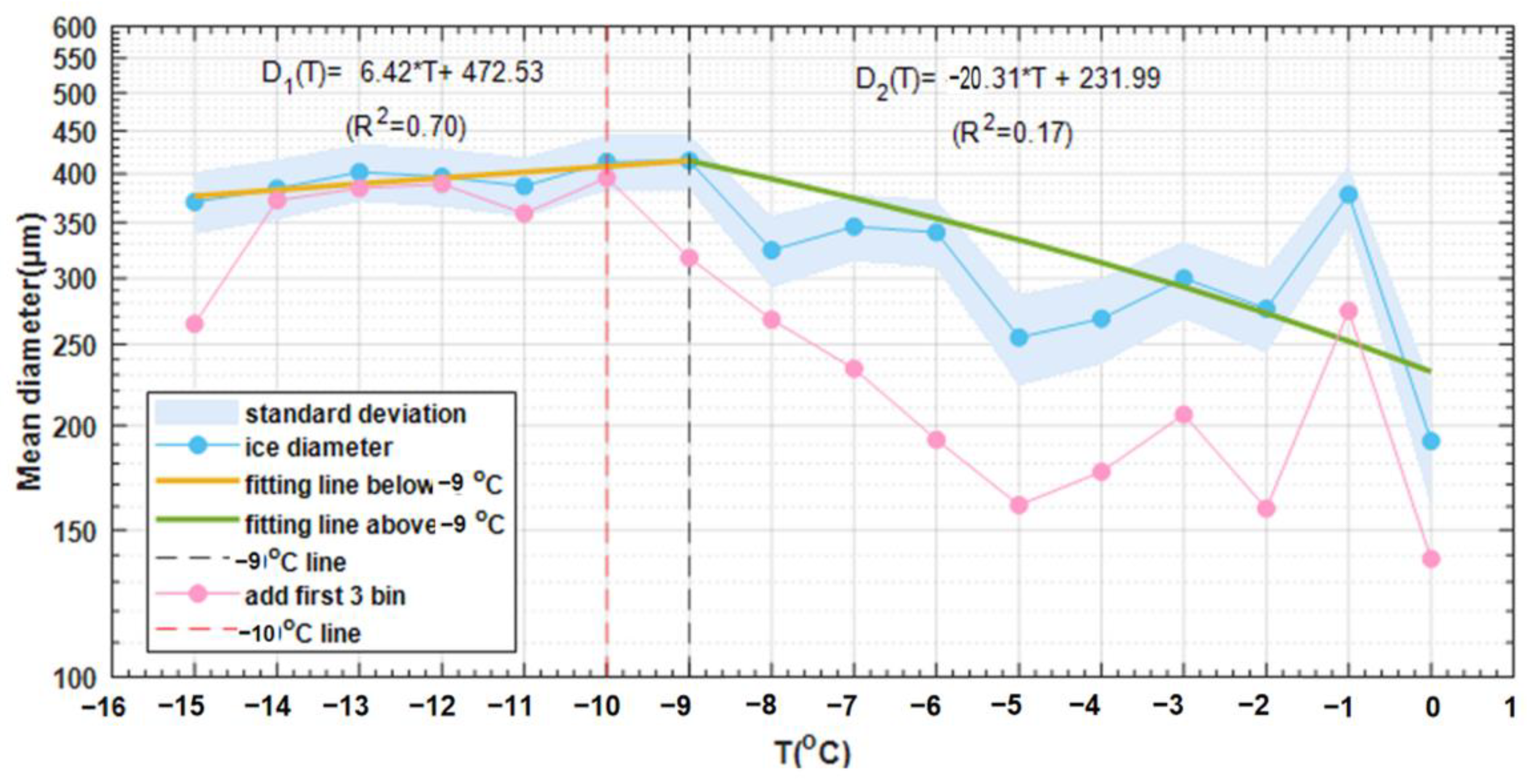
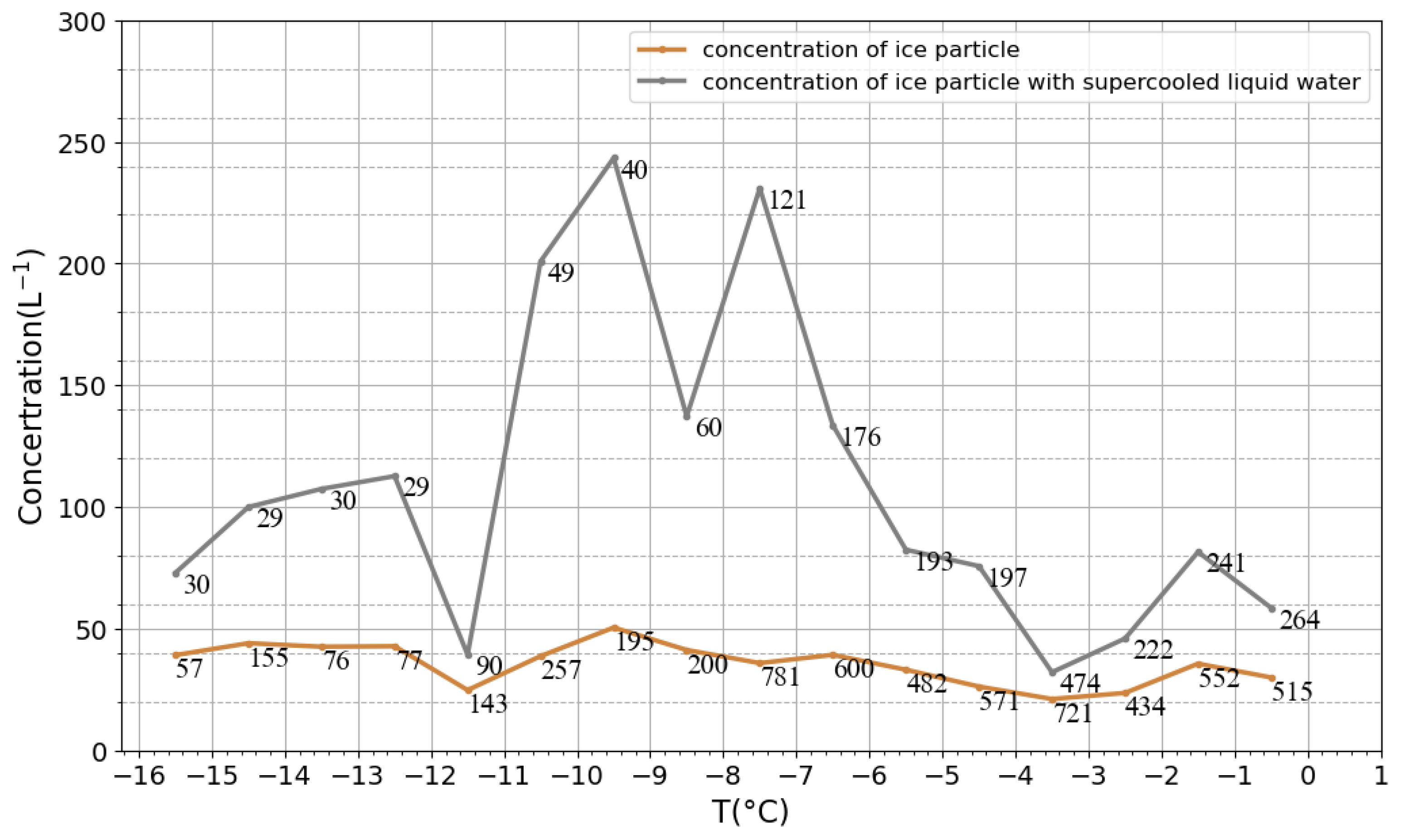
3. Analysis and Results

The ice PSDs at different temperatures were analyzed by dividing the temperature into four bins: −24–−20 °C (grey dot), −20–−16 °C (brown dot), −16–−12 °C (cyan dot), −12–−8 °C (blue dot), −8–−4 °C (yellow dot), and −4–0 °C (purple dot), based on the 29 aircraft observations, with the results shown in Figure 3a. The ice PSD averaged over the whole temperature range from −24 to 0 °C (red dot) is also shown in Figure 3. Figure 3a shows that there are more ice particles concentrated at the size range of 100–200 µm for all different temperature ranges. This is likely associated with the small sizes of ice particles, which mainly form via deposition and grow slowly, making the concentration relatively large. Similar ice PSDs are found for clouds with temperatures from −24 to −12 °C, as shown in Figure 3a. Moreover, there are also similar ice PSDs for clouds with temperatures from −8 to −4 °C and −4 to 0 °C. Figure 3a suggests that −12–−8 °C is a special temperature range for the spectral distribution of ice crystals, with high concentrations of ice particles with sizes greater than 400 µm. Particularly, there are higher concentrations of ice crystals with sizes greater than about 700 µm at a temperature range from −12 to −8 °C than at other temperature ranges. Thus, −8–−12 °C is roughly a threshold interval temperature: different ice PSDs of clouds exist for temperatures above and below this threshold interval value. The ice particle concentration is higher at the size range between 200 and 500 μm for clouds with temperatures below the threshold interval values than with temperatures above the threshold interval values, while it is similar at other size ranges. This is most likely related to the variation in ice nuclei (IN) concentrations with temperature [62], along with the growth rates of ice particles by deposition [63]. As known, when the temperature decreases every 4 °C, the IN concentration could increase by one order of magnitude [62]. At the same time, the growth of ice particles would consume water vapor, reduce the supersaturation, and cause the growth rate of ice particles to decrease. Moreover, the growth rate of large ice particles is inversely proportional to the particle diameter. Combined together, the above mentioned three factors likely make the ice particles within the size range between 200 and 500 µm for clouds with temperatures below −8–−12 °C much larger.
In order to study the effect of supercooled water on ice crystal distribution, especially in the temperature range from −8 to −12 °C, we analyzed the ice crystal distribution when T < 0 °C, FSSP-N > 10 cm−3 and FSSP-LWC > 0.001 g/m3 as the conditions containing more supercooled water, and the results are shown in Figure 3b. The most pronounced change in Figure 3b compared to Figure 3a is from −12 to −8 °C (blue dot), where the particle concentration with sizes of 200–400 µm is the lowest in all temperature ranges, along with a significant increase in particle concentration with sizes greater than 600 µm. This phenomenon is most likely the result of the Bergeron process with the involvement of supercooled water. A significant decrease in ice particle concentrations in the range of 100–600 µm can also be seen from −16 to −8 °C.
We further carried out an empirical fitting analysis of the ice PSD using both Gamma function and exponential function based on the 29 aircraft observations at different temperature ranges. Figure 4 shows both the empirical fitting (both Gamma and exponential) and observational ice PSDs averaged for different temperature ranges. Since the last four data samples at each temperature interval are too scattered with large uncertainties, they were not considered during the fitting analysis. The corresponding fitting parameters and observation-based evaluation (R2 and root mean square difference RMSE) results of ice PSDs are summarized in Table 2. It is clear that the Gamma fitting and exponential fitting of ice PSDs agree with each other when ice particles are large, while differ more for small sizes of ice particles. In general, the exponential fitting shows better fitting results for our measurements. In terms of different temperature intervals, Gamma fitting performs better at temperatures below −12 °C and exponential fitting performs better at temperatures above −12 °C. While parametrizations already exist in the literature, there are no parameterizations found for the study area we investigate here. The findings here could serve as a good reference for future ice particle size distribution parameterization over the study region. Thus, we did not compare their relative performance in the current study while a comparison study could be highly valuable in future with more observations including both particle size distributions and ice particle shapes.
To better understand the change of mean ice particle size with temperature, which is broadly used in the remote sensing study and radiative forcing study, Figure 5 shows the relationship between the average diameter of ice particles and temperature based on the statistical analysis of the 29 aircraft observations. Due to the small sample size at temperatures below −16 °C, we only studied the particle size distribution at the temperature range of −16–0 °C. Note that the temperature was binned with a step of −1 °C from 0 to −24 °C by using the upper border of temperature as the representative value. Both the average (blue line) and standard deviation (shaded area) of ice particle diameters at each temperature bin are shown in Figure 5. It shows a clear trend of ice particle mean diameter with temperature, which increases first and then decreases with temperature with the turning point at the temperature of −9 °C. This variation trend should be related to the difference of water vapor saturation pressure between ice and water. Previous studies have shown that the differences of water vapor saturation pressure between ice and water increases first and then decreases with temperature, with the maximum value at a temperature of around −12 °C [64]. If the clouds include both water (supercooled liquid droplets) and ice, the water evaporates and ice grows with the maximum growth rate around −12 °C [65,66], making the ice particles the largest around this temperature. If the clouds only include ice particles, the ice particles grow by deposition process, which is generally dependent on both the supersaturation and availability of water vapor. Considering that the supersaturation generally decreases with increasing temperature while water vapor amount increases [67], the growth rate of ice particles could reach a maximum value at a medium temperature while its exact value is unknown. Of course, the growth of ice particles also depends on the water supply from air below the clouds, which is beyond the scope of this study. Combining the two cases (with and without supercooled liquid droplets) mentioned above, the ice particle size should increase first and then decrease with temperature, with the maximum value occurring at a certain temperature that is most likely close to −12 °C.
By considering the ice particles with size ranges of 100–1600 µm, we calculated the mean diameters at different temperature ranges and investigated their relationship with temperature using linear fitting. As shown in Figure 5, the yellow solid line is the fitting line for temperatures below −9 °C, and the green solid line is the fitting line for temperatures above −9 °C. Note that the fitting equations and R2 are indicated in Figure 5. By considering the ice particles with size ranges of 25–1600 µm, we also calculated the mean diameters at different temperature ranges and investigated their relationship with temperature (pink line in Figure 5). Note that the ice particles with size ranges of 25–100 µm are obtained from the Gamma fitting. It is clear that the ice particle mean diameter shows a similar variation trend with temperature as that without considering the size range of 25–100 µm, but with the turning point changed from −9 to −10 °C. As expected, the ice particles sizes all become smaller by considering the ice particles with sizes below 100 µm, while the reduction is larger in the high-temperature zone.
We further investigated the relationship between ice particle concentration and temperature using the 29 aircraft observations, and the results are shown in Figure 6. The results show the change of ice particle concentration averaged in each temperature bin with temperature. The orange line represents the concentration of the ice particles at different temperatures, and the black line represents the concentration of ice particles with supercooled liquid droplets at different temperatures. The numbers of samples at different temperature ranges are also indicated in Figure 6. From 0 to −9 °C, the ice particle concentration increases from 13.37 to 50.23 L−1, with an average of 31.27 L−1. When supercooled liquid droplets coexist, the ice particle concentration is high at temperatures from −11 to −6 °C, which may be related to the aforementioned saturation factor. It also shows that the ice particle concentration is relatively small at a temperature range between −16 and −12 °C. On one hand, the lower the temperature, the less water vapor is supplied, which causes the relatively low ice particle concentration. On the other hand, the small number (29) of flights investigated in this study may also affect the observation results we found, introducing large potential uncertainties. However, the specific reasons need to be further explored in future.

4. Summary

By investigating the ice PSDs obtained from 29 aircraft observations in 2008, 2009, and 2013, we found that many ice particles are concentrated in the small size range and the ice PSD does not differ greatly for the size range between 100 and 200 μm. This is most likely associated with the slow deposition growth of ice particles, which generally differs little at different temperatures.
The temperature at −8–−10 °C can be used as a cut-off point when studying the properties of ice particles where temperature needs to be taken into account. When the temperature is lower than −8–−10 °C, the low temperature is conducive to the nucleation of ice crystals. The concentrations of ice particles between 200 and 600 μm have a high concentration of nucleation. Because of this, water vapor is consumed here, limiting the growth of ice crystals at 600–1600 μm.
The differences between the two fittings appear mainly in the fitting of ice particles smaller than 300 μm. In terms of different temperature intervals, this study shows that Gamma fitting performs better at temperatures below −12 °C and exponential fitting works better at temperatures above −12 °C. Thus, different fitting methods are suggested for different temperature intervals.
The trend in the mean diameter of ice particles (100–1550 μm) can be clearly divided into two parts with a turning point at a temperature of −9 °C. Shortly, the mean diameter increases with temperature from −15 to −9 °C, and decreases with temperature from −9 to 0 °C. This is most likely associated with the supersaturation differences between ice and water. Further analysis of the variation in mean diameter of ice particles (25–1550 μm), in which the ice particle concentrations of the first three bins (25–50, 50–75, and 75–100 µm) are calculated using the Gamma fitting, shows a similar finding while with the turning point changed from −9 to −10 °C. We also investigated the change of ice particle concentration with temperature. For pure ice clouds, the ice particle concentration also peaks at temperatures around −9 or −10 °C, with relatively weak variation with temperature. When there are supercooled liquid droplets coexisting, the ice particle concentration shows much higher values from −11 to −6 °C, which may be related to the aforementioned saturation factor. These findings demonstrate the importance of temperature for ice particles larger than 200 μm and reveal the turning point of temperature (−8–−10 °C) for the dependence of mean ice particle diameters on temperature.

Author Contributions

Methodology, S.L., C.Z.; writing—original draft preparation, S.L.; writing—review and editing, C.Z., Y.Z.; data—collecting, Y.Z., Z.W.; suggestion—theoretical guidance, Z.H. All authors have read and agreed to the published version of the manuscript.

Funding

This work was supported by the Ministry of Science and Technology of China National Key R&D Program (2017YFC1501403), the National Natural Science Foundation of China (41925022), the Hebei social development science and Technology Division (20375402D), and the State Key Laboratory of Earth Surface Processes and Resource Ecology.

Institutional Review Board Statement

Not applicable.

Informed Consent Statement

Not applicable.

Data Availability Statement

The data used in this study are available via https://pan.bnu.edu.cn/l/BF2gYn (Last access: 13 December 2021).

Conflicts of Interest

The authors declare no conflict of interest.

References

  1. Kinne, S.; Liou, K.N. The effects of the non-sphericity and size distribution of ice crystals on the radiative properties of cirrus clouds. Atmos. Res. 1989, 24, 273–284. [Google Scholar] [CrossRef]
  2. Liou, K.N.; Takano, Y. Light scattered by non-spherical particles: Remote sensing and climate implications. Atmos. Res. 1994, 31, 271–298. [Google Scholar] [CrossRef]
  3. Mason, B.J. The shapes of snow crystals-Fitness for purpose? Q. J. R. Meteorol. Soc. 1994, 120, 849–860. [Google Scholar]
  4. Zhang, Y.; Macke, A.; Albers, F. Effect of crystal size spectrum and crystal shape on stratiform cirrus radiative forcing. Atmos. Res. 1999, 52, 59–75. [Google Scholar] [CrossRef]
  5. Heymsfield, A.J. Properties of tropical and midlatitude ice cloud particle ensembles—Part II: Applications for mesoscale and climate models. J. Atmos. Sci. 2003, 60, 2592–2611. [Google Scholar] [CrossRef]
  6. Hu, Z.; He, G. Numerical simulation of microphysical processes in cumulonimbus, Part I: Microphysical model. Acta Meteorol. Sin. 1988, 2, 471–489. [Google Scholar]
  7. Baker, M.B. Cloud microphysics and climate. Science 1997, 276, 1072–1078. [Google Scholar] [CrossRef]
  8. Stephens, G.L.; Webster, P.J. Clouds and climate: Sensitivity of simple systems. J. Atmos. Sci. 1981, 38, 235–247. [Google Scholar] [CrossRef]
  9. Evans, A.G.; Locatelli, J.D.; Stoelinga, M.T.; Hobbs, P.V. The IMPROVE-1 storm of 1–2 February 2001. Part II: Cloud structures and the growth of precipitation. J. Atmos. Sci. 2005, 62, 3456–3473. [Google Scholar] [CrossRef]
  10. Baker, M.B.; Peter, T. Small-scale cloud processes and climate. Nature 2008, 451, 299–300. [Google Scholar] [CrossRef]
  11. Schiller, C.; Krämer, M.; Afchine, A.; Spelten, N.; Sitnikov, N. The ice water content of Arctic, mid latitude and tropical cirrus. J. Geophys. Res. 2008, 113, 1208–1245. [Google Scholar]
  12. Zhao, C.; Xie, S.; Klein, S.A.; Protat, A.; Shupe, M.D.; McFarlane, S.A.; Comstock, J.M.; Delanoe, J.; Deng, M.; Dunn, M.; et al. Toward Understanding of Differences in Current Cloud Retrievals of ARM Ground-based Measurements. J. Geophy. Res. 2012, 117, D10206. [Google Scholar] [CrossRef]
  13. Zhao, C.; Chen, Y.; Li, J.; Letu, H.; Su, Y.; Chen, T.; Wu, X. 15-year statistical analysis of cloud characteristics over China using Terra and Aqua MODIS observations. Int. J. Climatol. 2019, 38, 2612–2629. [Google Scholar] [CrossRef]
  14. King, M.D.; Platnick, S.; Menzel, W.P.; Ackerman, S.A.; Hubanks, P.A. Spatial and temporal distribution of clouds observed by MODIS onboard the Terra and Aqua satellites. IEEE Trans. Geosci. Remote Sens. 2013, 51, 3826–3852. [Google Scholar] [CrossRef]
  15. Rangno, A.L.; Hobbs, P.V. Ice particles in stratiform clouds in the Arctic and possible mechanisms for the production of high ice concentrations. J. Geophys. Res. 2001, 106, 15065–15075. [Google Scholar] [CrossRef]
  16. You, L.; Xiong, G.; Gao, M.; Lu, Y.; Sun, K.; Ren, D. The characteristics of ice crystal formation and snow growth processes of in spring stratiform clouds in Jilin Province. Acta Meteorol. Sin. 1965, 35, 423–433. (In Chinese) [Google Scholar]
  17. Delanoë, J.; Protat, A.; Testud, J.; Bouniol, D.; Forbes, R.M. Statistical properties of the normalized ice particle size distribution. J. Geophys. Res. Atmos. 2005, 110, 10201–10223. [Google Scholar] [CrossRef] [Green Version]
  18. Heymsfield, A.J.; Schmitt, C.; Bansemer, A. Ice cloud particle size distributions and pressure-dependent terminal velocities from in situ observations at temperatures from 0 to −86 °C. J. Atmos. Sci. 2013, 70, 4123–4154. [Google Scholar] [CrossRef]
  19. Yuan, F.; Lei, H.C. Aircraft observation of cloud microphysical characteristics of pre-stratiform-cloud precipitation in Jiangxi province. Atmos. Ocean. Sci. Lett. 2017, 10, 364–371. [Google Scholar]
  20. Yang, J.; Lei, H.; Hu, Z.; Hou, T. Particle size spectra and possible mechanisms of high ice concentration in nimbostratus over Hebei province, China. Atmos. Res. 2014, 142, 79–90. [Google Scholar] [CrossRef]
  21. Zhen, Z.; Lei, H. Observed microphysical structure of nimbostratus in northeast cold vortex over China. Atmos. Res. 2014, 142, 91–99. [Google Scholar]
  22. Li, T.L.; Bin, Y.; Guo, X.L.; Shao, Z.P. Analysis on the macro and micro physical characteristics of stratiform cloud in Henan. Meteorol. Environ. Res. 2010, 1, 96–100. [Google Scholar]
  23. Hou, T.; Lei, H.; Hu, Z. A comparative study of the microstructure and precipitation mechanisms for two stratiform clouds in China. Atmos. Res. 2010, 96, 447–460. [Google Scholar] [CrossRef]
  24. Hou, T.; Lei, H.; Hu, Z.; Zhou, J. Aircraft observations of ice particle properties in stratiform precipitating clouds. Adv. Meteorol. 2014, 2014, 1–12. [Google Scholar] [CrossRef]
  25. Zhu, S.; Guo, X.; Lu, G.; Li, J. Ice crystal habits and growth processes in stratiform clouds with embedded convection examined through aircraft observation in northern China. J. Atmos. Sci. 2015, 72, 2011–2032. [Google Scholar] [CrossRef]
  26. Zhao, C.; Zhao, L.; Dong, X. A case study of stratus cloud properties using in situ aircraft observations over Huanghua, China. Atmosphere 2019, 10, 19. [Google Scholar] [CrossRef] [Green Version]
  27. Strapp, J.W.; Albers, F.; Reuter, A.; Korolev, A.V.; Maixner, U.; Rashke, E.; Vukovic, Z. Laboratory measurements of the response of a PMS OAP-2DC. J. Atmos. Oceanic Technol. 2001, 18, 1150–1170. [Google Scholar] [CrossRef]
  28. Knollenberg, R.G. The optical array: An alternative to scattering or extinction for airborne particle size determination. J. Appl. Meteorol. 1970, 9, 86–103. [Google Scholar] [CrossRef]
  29. Mcfarquhar, G.M.; Cober, S.G. Single-scattering properties of mixed-phase Arctic clouds at solar wavelengths: Impacts on radiative transfer. J. Clim. 2004, 17, 3799–3813. [Google Scholar] [CrossRef]
  30. Mcfarquhar, G.M.; Zhang, G.; Poellot, M.R.; Kok, G.L.; Mccoy, R.; Tooman, T.; Fridlind, A.; Hemsfield, A.J. Ice properties of single-layer stratocumulus during the mixed-phase Arctic cloud experiment. I: Observations. J. Geophys. Res. Atmos. 2007, 112, 1201–1224. [Google Scholar] [CrossRef] [Green Version]
  31. Burnet, F.; Brenguier, J.L. Comparison between standard and modified forward scattering spectrometer probes during the small cumulus microphysics study. J. Atmos. Ocean. Technol. 2010, 19, 1516–1531. [Google Scholar] [CrossRef]
  32. Yang, Y.; Zhao, C.; Dong, X.; Fan, G.; Zhou, Y.; Wang, Y.; Zhao, L.; Lv, F.; Yan, F. Toward understanding the process-level impacts of aerosols on microphysical properties of shallow cumulus cloud using aircraft observations. Atmos. Res. 2019, 221, 27–33. [Google Scholar] [CrossRef]
  33. Jensen, E.J.; Lawson, P.; Baker, B.; Pilson, B.; Mo, Q.; Heymsfield, A.J.; Bansemer, A.; Bui, T.P.; McGill, M.; Hlavka, D.; et al. On the importance of small ice crystals in tropical anvil cirrus. Atmos. Chem. Phys. 2009, 9, 5519–5537. [Google Scholar] [CrossRef] [Green Version]
  34. McFarquhar, G.M.; Finlon, J.A.; Stechman, D.M.; Wu, W.; Jackson, R.C.; Freer, M. University of Illinois/Oklahoma Optical Array Probe (OAP) Processing Software; Zenodo: Genève, Switzerland, 2018. [Google Scholar] [CrossRef]
  35. Claffey, K.J.; Jones, K.F.; Ryerson, C.C. Use and Calibration of Rosemount Ice Detectors for Meteorological Research. Atmos. Res. 1995, 36, 277–286. [Google Scholar] [CrossRef]
  36. Cober, S.G.; Isaac, G.A.; Strapp, J.W. Aircraft Icing Measurements in East Coast Winter Storms. J. Appl. Meteorol. 1995, 34, 88–100. [Google Scholar] [CrossRef] [Green Version]
  37. Rangno, A.L.; Hobbs, P.V. Microstructures and precipitation development in cumulus and small cumulonimbus clouds over the warm pool of the tropical Pacific Ocean. Q. J. R. Meteorol. Soc. 2005, 131, 639–673. [Google Scholar] [CrossRef]
  38. Gultepe, I.; Isaac, G.A.; Leaitch, W.R.; Banic, C.M. Parameterization of marine stratus microphysics based on in situ observations: Implications for GCMs. J. Clim. 1996, 9, 345–357. [Google Scholar] [CrossRef] [Green Version]
  39. Gultepe, I.; Isaac, G.A. Aircraft observations of cloud droplet number concentration: Implications for climate studies. Q. J. R. Meteorol. Soc. 2004, 130, 2377–2390. [Google Scholar] [CrossRef]
  40. Zhang, Q.; Quan, J.; Tie, X.; Huang, M.; Ma, X. Impact of aerosol particles on cloud formation: Aircraft measurements in China. Atmos. Environ. 2011, 45, 665–672. [Google Scholar] [CrossRef]
  41. Cober, S.G.; Isaac, G.A.; Korolev, A.V. Assessing cloud-phase conditions. J. Appl. Meteorol. Clim. 2001, 40, 1967–1983. [Google Scholar] [CrossRef]
  42. Wang, L.J.; Yin, Y.; Yao, Z. Microphysical responses to catalysis during a stratocumulus aircraft seeding experiment over the Sanjiangyuan region of China. J. Meteorol. Res. 2014, 27, 849–867. [Google Scholar] [CrossRef]
  43. Liu, Y.; You, L.; Yang, W.; Liu, F. On the size distribution of cloud droplets. Atmos. Res. 1995, 35, 201–216. [Google Scholar] [CrossRef]
  44. Best, A.C. Dropsize distribution in cloud and fog. Q. J. R. Meteorol. Soc. 1951, 77, 418–426. [Google Scholar] [CrossRef]
  45. Kosarev, A.L.; Mazin, I.P. An empirical model of the physical structure of upper-layer clouds. Atmos. Res. 1991, 26, 213–228. [Google Scholar] [CrossRef]
  46. Levin, L.M. On the size distributions functions of the cloud and rain droplets. Dokl. Acad. Sci. USSR 1954, 44, 1045–1049. [Google Scholar]
  47. Deirmendjian, D. Scattering and polarization properties of water clouds and hazes in the visible and infrared. Appl. Opt. 1964, 3, 187–196. [Google Scholar] [CrossRef]
  48. Tampieri, F.; Tomasi, C. Size distribution models of fog and cloud droplets in terms of the modified gamma function. Tellus 1976, 28, 333–347. [Google Scholar] [CrossRef] [Green Version]
  49. Schumann, T.E.W. Theoretical aspects of the size distribution of fog particles. Q. J. R. Meteorol. Soc. 2010, 66, 195–208. [Google Scholar] [CrossRef]
  50. Ivanova, D.; Mitchell, D.L.; Arnott, W.P.; Poellot, M. A gcm parameterization for bimodal size spectra and ice mass removal rates in mid-latitude cirrus clouds. Atmos. Res. 2001, 59, 89–113. [Google Scholar] [CrossRef]
  51. Liu, Y.; Hallett, J. The “1/3” power-law between effective radius and liquid-water content. Q. J. R. Meteorol. Soc. 1997, 123, 1789–1795. [Google Scholar]
  52. Costa, A.A.; Oliveira, C.J.; Oliveira, J.C.P.; Sampaio, A.J.C. Microphysical observations of warm cumulus clouds in CEARA, Brazil. Atmos. Res. 2000, 54, 167–199. [Google Scholar] [CrossRef]
  53. Liu, Y.; Daum, P.H. Spectral dispersion of cloud droplet size distributions and the parameterization of cloud droplet effective radius. Geophys. Res. Lett. 2000, 27, 1903–1906. [Google Scholar] [CrossRef]
  54. Khrgian, A.K.; Mazin, I.P. Analysis of methods of characterization of distribution spectra of cloud droplets. Tr. TsAo. 1952, 7, 92–126. [Google Scholar]
  55. Heymsfield, A.J.; Platt, C.M.R. A parameterization of the particle size spectrum of ice clouds in terms of the ambient temperature and the ice water content. J. Atmos. Sci. 1984, 41, 846–855. [Google Scholar] [CrossRef] [Green Version]
  56. Arnott, W.P.; Dong, Y.Y.; Hallett, J. Role of small ice crystals in radiative properties of cirrus: A case study, FIRE II, 22 November 1991. J. Geophys. Res. 1994, 99, 1371–1381. [Google Scholar] [CrossRef]
  57. Mcfarquhar, G.M.; Heymsfield, A.J. Parameterization of tropical cirrus ice crystal size distributions and implications for radiative transfer: Results from CEPEX. J. Atmos. Sci. 1997, 54, 2187–2200. [Google Scholar] [CrossRef]
  58. Platt, C.M.R. A parameterization of the visible extinction coefficient of ice clouds in terms of the ice/water content. J. Atmos. Sci. 1997, 54, 2083–2098. [Google Scholar] [CrossRef]
  59. Puechel, R.F.; Hallett, J.; Strawa, A.W.; Howard, S.D.; Ferry, G.V.; Foster, T.; Arnott, W.P. Aerosol and cloud particles in tropical cirrus anvil: Importance to radiation balance. J. Aerosol Sci. 1997, 28, 1123–1136. [Google Scholar] [CrossRef]
  60. Ryan, B.F. A bulk parameterization of the ice particle size distribution and the optical properties in ice clouds. J. Atmos. Sci. 2000, 57, 1436–1451. [Google Scholar] [CrossRef]
  61. Gunn, K.L.S.; Marshall, J.S. The distribution with size of aggregate snowflakes. J. Atmos. Sci. 1958, 15, 452–461. [Google Scholar] [CrossRef] [Green Version]
  62. Che, Y.; Zhang, J.; Zhao, C.; Fang, W.; Xue, W.; Yang, W.; Ji, D.; Dang, J.; Duan, J.; Sun, J.; et al. A study on the characteristics of ice nucleating particles concentration and aerosols and their relationship in spring in Beijing. Atmos. Res. 2020, 247, 105196. [Google Scholar] [CrossRef]
  63. Mertes, S.; Schwarzenbock, A.; Laj, P.; Wobrock, W.; Pichon, J.M.; Orsi, G.; Heintzenberg, J. Changes of cloud microphysical properties during the transition from supercooled to mixed-phase conditions during CIME. Atmos. Res. 2001, 58, 267–294. [Google Scholar] [CrossRef]
  64. Mason, B.J. The Physics of Clouds; Oxford University Press: Oxford, UK, 1971; 660p. [Google Scholar]
  65. Tribus, M. Physical view of cloud seeding. Science 1970, 168, 201–211. [Google Scholar] [CrossRef] [PubMed]
  66. Zettlemoyer, A.C. Microphysics of clouds and precipitation. J. Colloid Interface Sci. 1979, 70, 289–290. [Google Scholar] [CrossRef]
  67. Fukuta, N. Water supersaturation in convective clouds. Atmos. Res. 1993, 30, 105–126. [Google Scholar] [CrossRef]
Figure 1. Average particle size distribution with the five available in situ aircraft observations from FSSP (red solid line), 2DC (blue solid line), and 2DC with quality checking by UIOOPS software (blue dashed line).
Atmosphere 13 00200 g001
Figure 2. The flight tracks of 20 flights, with different colors indicating different aircraft observations. The aircraft flights are named with year, month, day, and flight serial. The red star represents Zhengding Airport where all flights took off.
Atmosphere 13 00200 g002
Figure 3. Average ice PSD in conditions (a) with pure ice particles and (b) containing supercooled water at different temperature ranges obtained from the statistical analysis of the 29 aircraft observations. The red dot represents the temperature from −24 to −0 °C; the grey dot represents the temperature from −24 to −20 °C; the brown dot represents the temperature from −20 to −16 °C; the cyan dot represents the temperature from −16 to −12 °C; the blue dot represents the temperature from −12 to −8 °C; the yellow dot represents the temperature from −8 to −4 °C; and the purple dot represents the temperature from −4 to 0 °C.
Atmosphere 13 00200 g003
Figure 4. The Gamma (red lines) and exponential fittings (black lines) of ice PSDs averaged at different temperature ranges from the statistical analysis of the 29 aircraft observations: (a) −24 to −20 °C, (b) −20 to −16 °C, (c) −16 to −12 °C, (d) −12 to −8 °C, (e) −8 to −4 °C, (f) −4 to 0 °C, and (g) −24 to 0 °C. The dot represents the average distributions of the ice particles in different temperatures from the statistical analysis of the 29 aircraft observations. The red dot represents the temperature from −24 to −0 °C; the grey dot represents the temperature from −24 to −20 °C; the brown dot represents the temperature from −20 to −16 °C; the cyan dot represents the temperature from −16 to −12 °C; the blue dot represents the temperature from −12 to −8 °C; the yellow dot represents the temperature from −8 to −4 °C; and the purple dot represents the temperature from −4 to 0 °C.
Atmosphere 13 00200 g004
Figure 5. The relationship between the mean diameter of the ice particles and temperature. The blue line along with the shaded area represents the mean diameter of the ice particles at different temperatures from the statistical analysis of the 29 aircraft observations, in which the shaded area shows the standard deviation at different temperatures. The −9 °C line (black dotted line) divides the fitting of statistical analysis of the observations into two parts: (1) the fitting below −9 °C (the yellow line), and D1(T) is its fitting equation; (2) the fitting above −9 °C (the green line), and D2(T) is its fitting equation. The pink line represents the mean diameter of the ice particles at different temperatures after adding the first three bins.
Atmosphere 13 00200 g005
Figure 6. The change of ice particle concentration averaged in each temperature bin with temperature. The orange line represents the concentration of the ice particles at different temperatures from the statistical analysis of the 29 aircraft observations; the black line represents the concentration of ice particles with supercooled liquid water at different temperatures. The numbers in the two lines corresponding to each point represent the number of investigated samples divided by 10,000.
Atmosphere 13 00200 g006
Table 1. The detailed information including flight number (named with year, month, day, and flight serial), season, flight time, ground temperature, maximum flight heights, cloud types, and measured PSD number for the 29 in situ aircraft observations in Hebei, China.
YearFlightSeasonFlight Time (Beijing Time)Ground
Temperature
(°C)
Highest
Height
(m)
CloudTotal Number
of PSDs
200820080408f1Spring12:23–12:39146000Stratus615
20080408f3Spring20:15–22:22166000Stratus2723
20080522f1Spring19:15–21:55136000Stratus1600
20080526f1Spring10:48–13:37136000Stratus280
20081005f1Autumn08:45–11:17116084Stratus1880
20081020f1Autumn19:47–22:07195500Stratus1219
20081021f1Autumn10:39–12:49163900Stratus870
20081022f1Autumn21:14–23:07135700Stratus672
200920090324f1Spring07:50–10:4623000Stratus3583
20090329f2Spring16:00–19:1884300Stratus1180
20090509f1Spring13:43–16:22275800Stratus2339
20090510f1Spring09:52–12:56146000Stratus965
20090514f1Spring14:24–17:07187000Stratus1173
20090908f1Autumn13:40–16:43176600Stratus634
20090928f1Autumn15:01–17:33146800Stratus1006
20091011f1Autumn10:08–13:07147000Stratus500
20091011f2Autumn16:06–18:22107000Stratus525
20091025f1Autumn15:01–17:37227000Stratus604
201320130404f1Spring14:40–17:35166000Stratus5103
20130404f2Spring20:50–23:22187000Stratus941
20130419f1Spring09:40–12:33156400Stratus5043
20130921f1Autumn11:30–14:18167000Stratus4001
20130921f2Autumn16:55–18:45186800Stratus537
20130922f1Autumn19:10–21:55157000Stratus1586
20130923f1Autumn10:28–13:28157000Stratus3177
20131013f1Autumn09:05–11:30187000Stratus1318
20131013f2Autumn19:33–23:01144800Stratus3250
20131014f1Autumn09:43–12:00136800Stratus1201
20131014f2Autumn14:17–17:24146400Stratus3678
Table 2. The fitting parameters and observation-based evaluation (R2 and root mean square difference RMSE) results of ice PSDs. The better fitting methods for different temperature ranges are marked in red in the table.
Temperature (°C)Exponential
n(D) = N0 exp(−λD)
Gamma
n(D) = N0Dµ exp(−λD)
N0λR2RMSEN0µλR2RMSE
−24–−200.38260.0053380.890.02270.0003860.00751.32530.710.0201
−20–−160.88510.0057830.780.06710.0002000.00841.61310.920.0194
−16–−121.03380.0050590.650.09830.0000340.00831.98660.700.0484
−12–−80.36140.0035960.510.04600.0000020.00742.35000.270.0433
−8–−40.27170.0037480.640.03280.0013730.00541.01580.380.0428
−4–00.19760.0031640.580.04500.0443750.00360.28700.490.0493
−24–00.26870.0035850.670.03540.0086630.00470.65980.480.0447
Publisher’s Note: MDPI stays neutral with regard to jurisdictional claims in published maps and institutional affiliations.

