Abstract
Solar flare effects (Sfe) are magnetic variations caused by solar flare events. They only show up in the illuminated hemisphere. Their detection is a difficult task because they do not have a definite pattern and, additionally, they must be separated from other magnetic perturbations. However, we attempted to automatize these detections by using two different strategies. The first strategy takes advantage of one of the Sfe characteristics, as they usually have a rapid rise, followed by a smooth decay, which typically produces a crochet-like shape in the magnetograms. Thus, we created several morphological models for each magnetic component. Then, we identified a definite Sfe time interval by setting the conditions for various parameters, such as the correlations of the measured data with the models, or the model similarities among the different components. In the second stage of this strategy, we observed clusters of time intervals. Each of these clusters were attributed to a timespan of event possibility. We found the statistical optimal value of the correlation parameters by using the ROC curve method and Youden index. The second strategy was based on some of the properties of Sfe ionospheric electric currents, such as their spherical symmetry around the vortex. Here, the algorithm calculated the derivative of the data in order to avoid contamination of the daily variation , and, by means of trigonometric formulas, computed the magnetic radial component relative to the Sfe current vortex (the focus). It then created an Sfe index with this data. A prior assumption of the focus position in a preceding work is no longer needed since we made a wide patrol of the space area to find it. Through a progressive thresholding process, we found its statistical optimal value (0.4 nT min−1) again by using the ROC curve method and Youden index. For both of the strategies, we have made a large calculation of Sfe detection (for the period of 2000–2020), which included 33 Sfe. Finally, we combined the results of both methods—which in fact are complementary—and obtained a unified list that gave a higher hit ratio than those that were obtained separately. This unified method gave promising results towards the possibility of Sfe automatic detection.
1. Introduction
Sfe are rapid magnetic variations that arise when extra ionizing radiation reaches the Earth. They are essentially linked to solar flares [1]. Flares cause disturbances in the ionosphere, activating several layers, and creating technological problems associated with the absorption and delay of radio signals [2]. At the same time, electric currents generated at about 100 km high, produce induced magnetic fields that map on the magnetograms as what we call Sfe. Very large Sfe rarely occur [3], but those with small and medium amplitudes are very common and their number follow the solar cycle. Due to the disturbances that these phenomena create on technological systems, they are of interest in space weather sciences and the IAGA commissioned the Ebro observatory to create annual lists of these events. They can be found on the Ebro web page (http://www.obsebre.es/en/rapid accessed on 27 December 2021) and the ISGI web page (http://isgi.unistra.fr/events_sfe.php, accessed on 27 December 2021). The procedure used to identify these events has evolved very little since the last century and relies on the ability of a group of observers, belonging to collaborating observatories distributed around the world, who scrutinize their magnetograms and try to identify Sfe footprints on them. This is not an easy task because of the lack of one clear morphology of Sfe. Therefore, some additional confirmation from other proxies is often necessary [4].
A first attempt to construct an algorithm to automatically detect Sfe was conducted by Curto et al. [5]. Their prototype was based on some of the properties of the Sfe vector configuration; in particular, a certain symmetry around the central point of the whirl of these ionospheric currents, which is called the focus. That prototype produced encouraging results, so we resumed this effort and looked deeper into the problem by improving the method and proposing a new alternative approach.
2. Morphological Model
As we said above, the traditional method of Sfe detection required the visual inspection of the magnetograms by skilled operators who tried to find the particular crochet-like shape of these events [6] on the magnetograms. However, this is not an easy task due to the varying morphology of Sfe, which depends on the position of the magnetic observatory at the time of the event with respect to the ionospheric current system that causes them [7,8]. Moreover, the temporal variations of the magnetic field during an Sfe depends on the variations that the ionizing radiations experience [9] and the state of the atmospheric constituents in the dynamo region that are the base of those currents [10,11].
Here, first of all, through statistical studies over a long data series, we extracted the most common features of these events in order to obtain morphological models, which could then be compared with the variations that we observed in the magnetograms. The period of analysis was 2000–2015, when, according to the Service of Rapid Magnetic Variations [12], 107 Sfe events were detected during the daytime at the Ebro observatory. The selected data used to construct the models were minute geomagnetic variations for the X, Y, Z, H, and F components.
For each Sfe event, we determined the starting and the ending times, then, we extracted the specific Sfe signature by subtracting the solar quiet (Sq) variation (Figure 1). In order to simplify the procedure, if the variation was negative, we mirrored it to the positive side, so we only had to handle one-way movements.
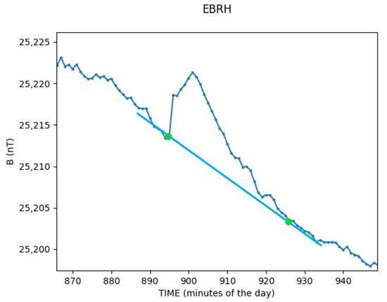
Figure 1.
H-component variation at Ebro observatory (EBR) for the day 28 September 2015 during an Sfe. Green dots represent the beginning and the end time of this event, having its start at the 895th minute of the day, which corresponds to 14:55 p.m., and the ending time at the minute 924, which corresponds to 15:25 p.m. The blue straight line is the interpolation used to compute the equivalent Sq variation that should be removed to isolate the Sfe variation.
At that point, we had a collection of different shapes that, initially, were not directly comparable because of their different amplitudes and durations. In order to standardize them, we divided the individual values of each event by its maximum value, then, we re-scaled them by dividing the time by its duration so that, at the end, we were able to represent the whole set of events with the same normalized axis, ranking from 0 to 1 (Figure 2).
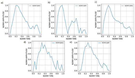
Figure 2.
Sfe variations at EBR corresponding to 28 September 2015 with the different magnetic components: (a) X component, (b) Y component (c) H component (d) Z component and (e) F component. All being represented in normalized axis.
In order to deal with the wide variety of shapes, we grouped them depending on the position of their maximum. For each component, four groups were established (Figure 3). Due to the initial different amplitudes and durations of the events, when they were represented on the standardized axes, they had a different number of points, so the points of one event do not necessarily coincide with those of another event. Thus, we interpolated each of them, thereby creating synthetic functions that allowed us to obtain, for each event, a homogenous number of points evenly distributed in that interval. Finally, we computed the mean value for each time slot.
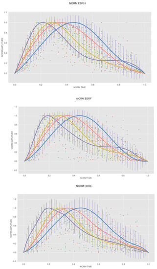
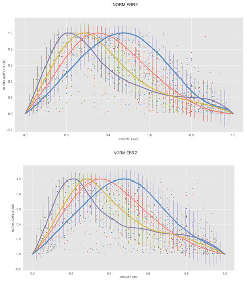
Figure 3.
Models corresponding to each one of the different magnetic components. Purple color relates to model 1, yellow color to model 2, red color to model 3, and blue color to model 4.
Table 1 displays the relative location of the maximum in the whole standardized duration and amplitude.

Table 1.
Relative location of the point of maximum for each of the four models.
Once the models had been established, to test the algorithm performance we compared the models with the real data in order to find the degree of matching. Again, we used EBR data as our benchmark. This time, we only used the days for the interval of 2000–2020 when EBR reported an Sfe or a very clear Sfe. Specifically, we analyzed 33 Sfe. But, here, new difficulties arose. A priori, the Sfe duration in the magnetogram was not known and, additionally, the Sfe variations were mixed in with other variations (for example the daily variation, Sq).
We proceeded as follows. For each daylight minute, we selected a set of possible time intervals, from 5 to 40 min spans (Figure 4). This represented a large load of computing (e.g., for a day with 12 h of light, we had the following: 12 h × 60 min/h × 36 intervals/min = 26,000 intervals to be processed for one day of data).
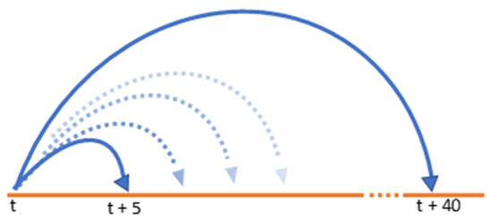
Figure 4.
Diagram showing the interval selection with durations ranging from 5 to 40 min.
For each interval of the real data, we repeated the treatment of standardization that we had conducted to obtain the models, in order for the data to be fully comparable with them. Then, we computed the correlation with each of the four models (Table 2). Among the calculated correlations, the highest one, and its corresponding model number, was selected.
Table 2.
Fragment of a table with intervals already analyzed. Each row contains the start and the end times, the time of the maximum for each component. Also, for each component the coefficient of correlation, and the model type that best adjusts with the data.
Once these results were compiled, we chose a variety of conditions involving the model type, the correlation value, the coherence among components, etc., then, we constructed several sets of conditions (see Table 3) to be imposed on the resulting data. The intervals that met the required conditions were assigned as candidates to be Sfe. With this, however, the final results of the detection were not fully satisfactory because we were only able to produce true positive percentages inferior to 50%.
Table 3.
Some sets of conditions used in the test procedure.
Then, we introduced a new scope for the problem. When observing the temporal evolution of the correlations, we found that a different behavior manifested under Sfe time, in contrast to the “quiet time” with no Sfe. In fact, when no Sfe occurred, the diagrams were chaotic and only some peaks of high correlations appeared (Figure 5a), while, if an Sfe was present, a certain order could be found (Figure 5b). In this case, a great number of rows corresponding to consecutive intervals with high correlation intervals formed a plateau, revealing that an Sfe was present. The periodic decreases correspond to a lack of alignment between the duration of the real data (containing an Sfe) and the duration of the proposed model.
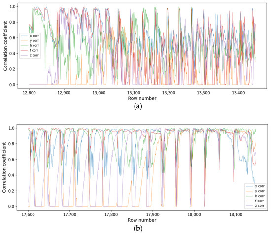
Figure 5.
(a): Plot showing the temporal behavior of the correlation coefficient against the corresponding time intervals identified by their row number. This plot corresponds to a time with no Sfe. A chaotic behavior is present. Each colored line corresponds to a different magnetic component. (b): Similar to Figure 5a, but for intervals belonging to Sfe time. Here, a series of periodic plateaus corresponding to consecutive intervals with high correlation are noticeable.
In general, among the different magnetic components, the module component, F, achieved the best correlations. So, this component was selected to apply the analysis in the algorithm.
In order to get rid of the background noise, the intervals were filtered, leaving only those with a correlation (r) above a certain threshold value (rmin). Only those intervals with a high correlation were considered as candidates for Sfe. We stabilized the lower limit at 0.970. After filtering the whole set of intervals, we had a list with the remaining intervals.
The next step was to find clusters of intervals that, having high correlations, also had similar starting and ending times. So, intervals with similar starting times were grouped together. For each interval, if there was more than 3 min difference between the starting time of this new interval and that of any established group, that interval was counted as a new group.
The algorithm promoted only those groups containing at least a certain number of intervals (9) as possible Sfe for a minimum duration. In this case, an Sfe alert was produced. The number of intervals in a group required to raise the alert was set as a variable N, with its lower limit at nine. Therefore, the final algorithm for automating Sfe detection depended on two variables whose optimal value was assessed through the following statistical analysis.
Figure 6 shows a segment of the analyzed data. Here, the two red lines point out the initial and the final times of the ordered behavior corresponding to an Sfe time. It includes 480 rows, which are equivalent to 13 min.
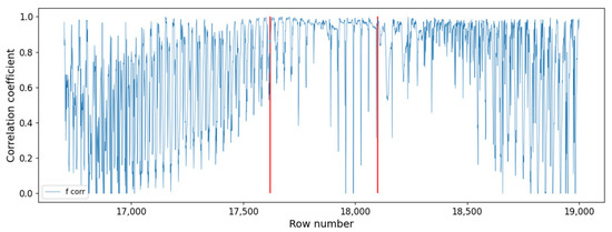
Figure 6.
Example of analysis of an ordered behavior corresponding to an Sfe. Red lines indicate the beginning and the end of this ordered section.
Finally, we looked at the statistics for the optimal threshold values of r and N. But first, some basic definitions of the terms we use are necessary [13]. In our case, TP are true Sfe detected by the algorithm, FN are true Sfe not detected by the algorithm, FP are candidates detected by the algorithm that are not Sfe, and TN are candidates dismissed by the algorithm that are not Sfe. To determine the TPR, TNR, and FPR, we used the following formulas:
TPR (True Positive Rate) = TP/(TP + FN)
TNR (True Negative Rate) = TN/((TN+FP)
FPR (False Positive Rate) = FP/(FP+ TN)
The first difficulty, then, was to unify the units. While the true positives, TP, accounted for hit Sfe events with a definite duration, the true negatives, TN, accounted for minutes with no Sfe. The imbalance between both of those numbers could bias the FPR and TPR rates, thus making the variations in TP irrelevant and underestimating FP. So, alternatively to time units (the first strategy), we handled the events by assigning a duration for TN. Two additional strategies were tested. In the second strategy, we took a standard length of 16 min per event. This was the median value for the Sfe duration according to a statistical analysis performed by Curto et al. [10] over 30 years of data. The third strategy was processed by taking the average length of all of the time intervals with Sfe as our reference duration. For these latter two strategiess, we divided the non-alert minutes by the reference duration. Thus, we obtained the number of events that could have caused an alert, but which had not since they were true negatives.
For the statistical work, we used ROC curves [14]. They are two-dimensional graphs, in which the true positives fraction (TPF) is represented on the Y-axis and the false positives fraction (FPF) is represented on the X-axis (Figure 7). They allow us to assess the relative balance between the benefits (the true positives) and the costs (the false positives). In the ROC curves, the optimal threshold is the one closest to the diagonal.
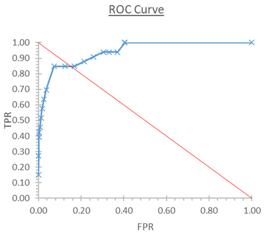
Figure 7.
ROC curve for Sfe detection with the morphological method using N = 22, which corresponds to the optimal value. The optimal thresholds values are those having, in this representation, the projected point closest to the diagonal.
In general, if the fraction of true positives (TPR) increases, the fraction of true negatives (TNR) decreases. In this situation, an acceptable compromise must be reached. One of the proposed solutions is to select the cut-off point that maximizes the difference between the fractions of true positives and false positives. The maximum value of this amount is the Youden index (YI) and the cut-off point—the point of the ROC curve corresponding to this index—is often selected as the optimal cut-off point of the marker [15].
Thus, the Youden index is as follows:
YI = TPR + TNR +1
Table 4 displays the numerical values achieved by each correlation threshold. Not showed here, N was also varied to obtain the best Youden index, for the optimal detection. The best results were obtained for the correlation threshold = 0.985 and N = 22. Thus, with these threshold values, we had 84.8% detection of Sfe. This is a good achievement. However, there were still too many false positives.
Table 4.
Youden index as a function of the correlation coefficient threshold (condition) for the three ways to compute negatives: minutes, mean duration, and 16 min duration. This is the trial for N = 22, which gives the best performance. Last columns give the resulting true positives, false positives, and false negatives.
3. Geometrical Model
Another approach to the Sfe detection problem involves taking advantage of some of the properties of Sfe ionospheric currents, especially their spherical symmetry around the vortex [16]. A first attempt was carried out by Curto et al. [5]. Their prototype algorithm calculated the derivative of the data in order to avoid contamination of the daily variation Sq, and, by means of trigonometric formulas, they computed the magnetic radial component. Finally, an Sfe index was created. Here, we followed the same steps but, to avoid the shortcomings of the former design, some improvements were implemented.
As mentioned previously, ideally, the electric circuit for Sfe has a circle-like shape flowing around a central point, which is the current vortex. The induced magnetic vectors point towards the center in the Northern Hemisphere (Figure 8) and away from it in the Southern Hemisphere [17]. In our case, we used data from observatories in the Northern hemisphere because they had a denser distribution. We limited them to those with latitudes ranging from 23° to 70° degrees in order to avoid contamination from both auroral and equatorial electrojets.
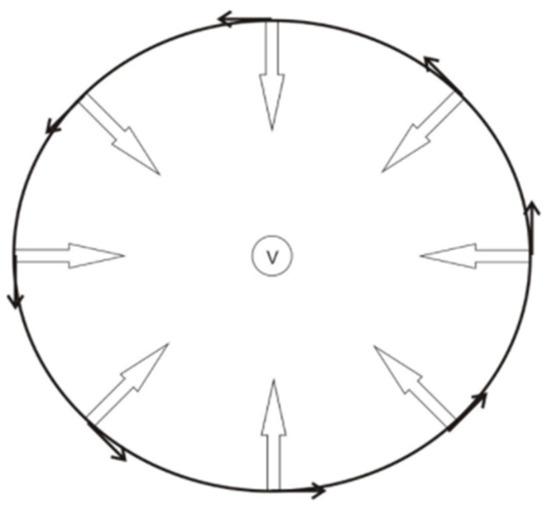
Figure 8.
Diagram of the electric circuit with Sfe currents (black arrows) and the induced magnetic vectors (white arrows). In the Northern hemisphere, electric currents circulate counterclockwise and magnetic vectors point towards the focus of the system (v).
Again, we performed a massive calculation for the days with Sfe events recorded in the period of 2000–2020. We only used the events confirmed by the International Service of Rapid Magnetic Variations [12] and reported by EBR as being clear or very clear. The minute data were obtained from observatories belonging to the INTERMAGNET network (https://www.intermagnet.org/data-donnee/data-eng.php accessed on 27 December 2021). Specifically, we analyzed 33 Sfe, the same days analyzed with the morphological method, but, here, we used data not only from EBR but also from other observatories in the lit hemisphere.
First of all, the magnetic data were filtered to avoid contamination of the daily variation Sq because Sfe are high frequency phenomena with respect to Sq. We used the derivative as a high-pass filter, as in Curto et al. [5], but in this case it was conducted with intervals of 8 min and not minute by minute, the option that was used in that first prototype. We used 8 min intervals because it was the average time of the Sfe events and the high frequency magnetic noise was better filtered. Sfe signals usually are a composition of step and ramp signals, but, after derivation, they become peaks and steps, respectively. In Figure 9, the magnetic data from the Belsk observatory in Poland (BEL) is displayed. It corresponds to 6 September 2017. According to the International Service of Rapid Magnetic Variations, on this day there was an Sfe at 12:00 p.m. In the left part of the figure (a), direct X and Y components of the magnetic field, without any filter, are shown and, in the right part (b), dX and dY, after the derivative filter, are shown. Thus, with that filter, the signal of the daily variation disappeared, and only that corresponding to the Sfe remained.
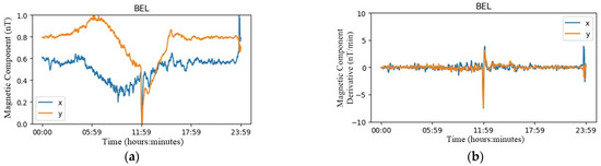
Figure 9.
Magnetic data of BEL observatory corresponding to 6 September 2017 before (a) and after (b) applying a high pass filter. Close to noon, an Sfe can be seen.
As said previously, in our analysis, we only used the data from the observatories in the illuminated hemisphere. Those observatories beyond the terminator do not contribute with useful signal and sometimes only add noise.
The second part of our algorithm performs a change in coordinates, computing at each observatory the radial component of the variation relative to a hypothetical center where the vortex could be located; details of which can be found in Curto et al. [5]. Contrary to the prototype that used a prefixed position of the vortex, here the position was varied by sweeping the space area to find the focus position. For each trial, we computed the vectorial addition of the radial component of the contributing observatories, divided by the number of observatories we used. So, a new index called the delta index was computed, as follows:
δSFET = (ΔBr1 +ΔBr2 + … + ΔBrn)/n
The trial obtaining the highest values of this index was identified and its corresponding central point was taken as the coordinates’ origin, being considered as the focus.
This process was repeated for every minute of the day. Figure 10 shows the evolution of this index for 5 December 2006. The big oscillation around 10:30 a.m. reveals the presence of an Sfe.
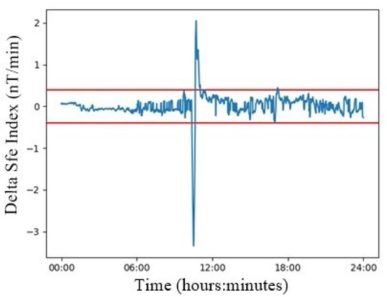
Figure 10.
Delta Sfe index for 5 December 2006 (blue line). A typical oscillation corresponding to an Sfe can be seen at 10:30 a.m. Red lines are the proposed threshold.
However, during any day, but specially on those days having disturbances, such as magnetic storms or sub-storms, there were plenty of small peaks in the delta index that were simply noise. So, we implemented a threshold (red lines in Figure 10) to discard that noise and to determine whether the algorithm should sound an alert about an Sfe or not. In order to obtain the optimal threshold value, we varied it between 0.1 and 1 nT/min, with increments of 0.1 nT/min. Then, in each trial we computed the number of strikes (true positives) but also the number of false positives. With those data, as in the previous chapter, we produced statistics and determined the optimal threshold in order to retain as much of the event as possible with minimum errors.
The Youden index tells us, numerically, the optimal condition for the threshold (Table 5). In our case, it was 0.4 nT/min. This is coincident with what we see in Figure 11. With this threshold, the geometrical method detects 28 out of 33 Sfe, which represents 84.8% of the existing ones, but, as a counterpart, at the same time it detects 162 FP events.
Table 5.
Youden index for the geometrical method using the correlation threshold values as the main condition.
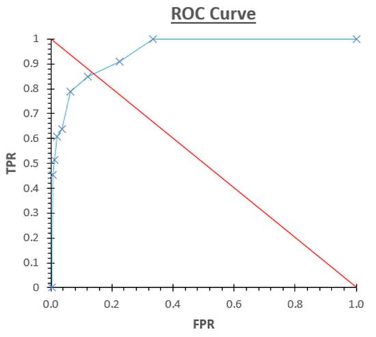
Figure 11.
ROC curve allowing us to monitor the optimal threshold selection. Red line represents the diagonal. The point closer to the (0.01) vertex and to that line represents the best option. In this case, the point closest to the diagonal corresponds to a threshold value of 0.4 nT/min.
4. Unified Model
It is clear that one model copes with some aspects that the other does not deal with, and vice versa, so both models are complementary. Given this, the next logical step was to combine both of the methods to try to obtain the best of both worlds and, in this way, achieve a higher hit ratio than the one obtained when working separately.
However, directly merging the individual lists into a unified one while maintaining the former thresholds, does not perhaps give the best possible results, so we performed a new optimization process varying the thresholds of both of the methods simultaneously in order to achieve the optimal detection.
In the first strategy, we worked with minutes, and, as we can see (Figure 12), with the maximum Youden index, we detected 31 out of 33 Sfe, but with 134 FP.
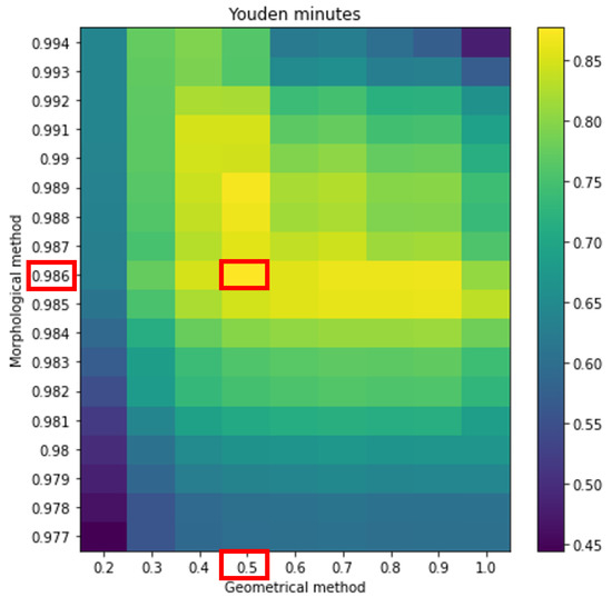
Figure 12.
Two-dimensional representation of Youden index as a function of the threshold conditions for both, the morphological and the geometrical methods when working in minutes. Red squares indicate the optimum values of the parameters and the peak value of the Youden index.
As mentioned previously, in the second strategy, we took a length of 16 min per event as the reference duration. In this case (Figure 13) we detected 31 Sfe and 97 FP.
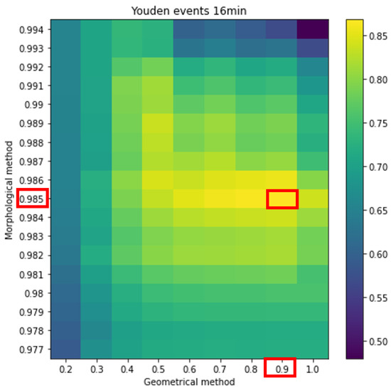
Figure 13.
The same as Figure 12 but taking as reference a length of 16 min per event.
Finally, we followed the same procedure as previously described but we took the average length of all of the time intervals with Sfe as the reference duration (Figure 14). And for this case, we obtained 30 Sfe and 72 FP. This was the best option because it drastically reduced FP without losing much TP and we chose it for the operative mode.
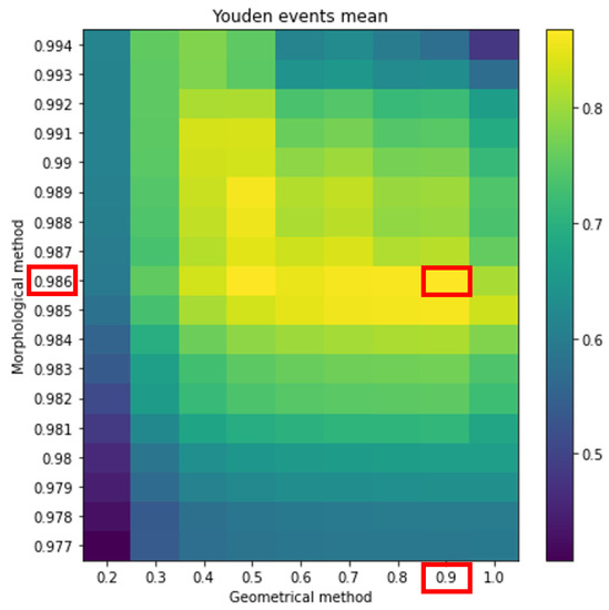
Figure 14.
The same as Figure 12 but taking as the reference the average length of all the time intervals having an Sfe.
We can summarize the performances of the different methods in Table 6.
Table 6.
Maximum scores of each different method. Their performance is summarized by the Youden index. Joint method overcomes the others.
It is clear that the performance of the joint method is the best, as pointed out by the Youden index. Figure 15 displays a flow chart with the main steps towards providing a reliable and comprehensive list of Sfe events.
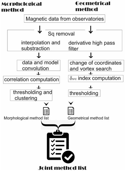
Figure 15.
Flow chart of the whole procedure, which ends with a list of Sfe candidates from the joint method.
5. Conclusions
Sfe detection is a complex and burdensome endeavor, so we produced a method to complete this task using algorithms designed to treat magnetic data unattended and massively. Our eventual aim was to have a method capable of doing this task automatically. At the beginning, two different methods were proposed. One, capturing the morphological characteristics of these events which was similar to the usual manual procedure conducted by collaborating observers looking closely the magnetograms to find movements that match the models extracted by the experience of previous events. The other method, taking advantage of some of the geometrical properties of the Sfe magnetic vectors, relied on a new index that was defined in a way such that its value increased in the presence of an Sfe. In both cases, we looked for the optimal values of the internal parameters involved in the Sfe selection. We used statistics, such as ROC curves and Youden indices, to achieve them. Both of these methods succeeded in giving useful lists of Sfe candidates. However, the lists were dissimilar but complementary. One list contained events that were lacking in the other list, and vice versa. So, we realized that there was room for improvement. That was achieved by joining both methods. With the two methods working separately, we had similar percentages of Sfe true detections (84.8%), but a different Youden index and FPR. However, when combining both of the methods, we achieved 90.9% true detections. In order to obtain this figure, we had to perform a similar statistical optimization process as we conducted when they worked separately, but this time the internal parameters of both of the methods were varied simultaneously to determine the best option. From the three strategies used to determine FN, we selected “time” and specifically “mean duration”. With this choice, compared to the “16 min duration” option, we saw a reduction of one in the numbers of true positives (TP) but, in contrast, we benefited from obtaining a reduction of 20 false positives (FP). Additionally, the Youden index was higher. And the minutes-way was discarded because it dramatically underestimated false positives.
To summarize, with this work we highly improved the performance of the former Sfe geometric detector prototype by combining it with a morphological method, which takes into account the shape of the movement in the magnetograms. This is something that human observers do routinely by eye when looking for these events and now we have incorporated it into the machine routine analysis. The joint method achieved high scores of success in detecting Sfe and will be of great help for the Service of Rapid Magnetic Variations to confirm Sfe candidates.
Author Contributions
Conceptualization and methodology, J.J.C.S.; software and validation, A.F.-C. and A.S.; formal analysis and data curation, A.F.-C. and A.S.; writing—original draft preparation, J.J.C.S., A.F.-C. and A.S.; supervision, J.J.C.S.; funding acquisition, J.J.C.S. All authors have read and agreed to the published version of the manuscript.
Funding
This research was funded by Ministerio de Ciencia, Innovación Y Universidades project number PGC2018-096774-B-I00.
Institutional Review Board Statement
Not applicable.
Informed Consent Statement
Not applicable.
Acknowledgments
This research has been partly supported by the Spanish project PGC2018-096774-B-I00 of MICIINUN. The authors also wish to thank INTERMAGNET and all the collaborating observatories providing high-quality magnetic data. Finally, we thank the International Service of Rapid Magnetic Variations and its collaborating observatories for providing lists of Sfe events.
Conflicts of Interest
The authors declare no conflict of interest.
References
- Curto, J.J. Geomagnetic solar flare effects: A review. J. Space Weather Space Clim. 2020, 10, 27. [Google Scholar] [CrossRef]
- Tsurutani, B.T.; Verkhoglyadova, O.P.; Mannucci, A.J.; Lakhina, G.S.; Li, G.; Zank, G.P. A brief review of “solar flare effects” on the ionosphere. Radio Sci. 2009, 44, RS0A17. [Google Scholar] [CrossRef]
- Curto, J.J.; Castell, J.; Del Moral, F. Sfe: Waiting for the big one. J. Space Weather. Space Clim. 2016, 6, A23. [Google Scholar] [CrossRef]
- Curto, J.J.; Juan, J.M.; Timoté, C.C. Confirming geomagnetic Sfe by means of a solar flare detector based on GNSS. J. Space Weather. Space Clim. 2019, 9, A42. [Google Scholar] [CrossRef]
- Curto, J.J.; Marsal, S.; Creci, G.; Domingo, G. Automatic detection of Sfe: A proposal. Ann. Geophys. 2017, 35, 799–804. [Google Scholar] [CrossRef][Green Version]
- Romañá, A. Provisional atlas of rapid variations. Ann. Int. Geophys. Year 1959, IIB, 668–709. [Google Scholar]
- Curto, J.J.; Gaya-Piqué, L.R. Geoeffectiveness of solar flares in magnetic crochet (sfe) production: I—Dependence on their spectral nature and position on the solar disk. J. Atmos. Sol.-Terr. Phy. 2009, 71, 1695–1704. [Google Scholar] [CrossRef]
- Curto, J.J.; Gaya-Piqué, L.R. Geoeffectiveness of solar flares in magnetic crochet (sfe) production: II—Dependence on the detection method. J. Atmos. Sol.-Terr. Phy. 2009, 71, 1705–1710. [Google Scholar] [CrossRef]
- Curto, J.J.; Alberca, L.F.; Castell, J. Dynamic aspects of the Solar Flare Effects and their impact in the detection procedure. J. Ind. Geophys. Union 2016, 2, 99–104. [Google Scholar]
- Curto, J.J.; Amory-Mazaudier, C.; Cardús, J.O.; Torta, J.M.; Menvielle, M. Solar flare effects at Ebre: Regular and reversed solar flare effects, statistical analysis (1953 to 1985), a global case study and a model of elliptical ionospheric currents. J. Geophys. Res. 1994, 99, 3945–3954. [Google Scholar] [CrossRef]
- Curto, J.J.; Amory-Mazaudier, C.; Cardús, J.O.; Torta, J.M.; Menvielle, M. Solar flare effects at Ebre: Unidimentional physical, integrated model. J. Geophys. Res. 1994, 99, 23289–23296. [Google Scholar] [CrossRef]
- Curto, J.J.; Cardús, J.O.; Alberca, L.F.; Blanch, E. Milestones of the IAGA International Service of Rapid Magnetic Variations. Earth Planets Space 2007, 59, 463–471. [Google Scholar] [CrossRef]
- Youden, W.J. Index for rating diagnostic tests. Cancer 1950, 3, 32–35. [Google Scholar] [CrossRef]
- Fawcett, T. An introduction to ROC analysis. Pattern Recognit. Lett. 2006, 27, 861–874. [Google Scholar] [CrossRef]
- Fluss, R.; Faraggi, D.; Reiser, B. Estimation of the Youden Index and its Associated Cutoff Point. Biom. J. 2005, 47, 458–472. [Google Scholar] [CrossRef] [PubMed]
- Curto, J.J.; Marsal, S.; Blanch, E.; Altadill, D. Analysis of the Solar Flare Effects of 6 September 2017 in the ionosphere and in the Earth’s magnetic field using spherical elementary current systems. Space Weather 2018, 16, 1709–1720. [Google Scholar] [CrossRef]
- Richmond, A.D.; Venkateswaran, S.V. Geomagnetic crochets and associated ionospheric current systems. Radio Sci. 1971, 6, 139–164. [Google Scholar] [CrossRef]


Publisher’s Note: MDPI stays neutral with regard to jurisdictional claims in published maps and institutional affiliations. |
© 2022 by the authors. Licensee MDPI, Basel, Switzerland. This article is an open access article distributed under the terms and conditions of the Creative Commons Attribution (CC BY) license (https://creativecommons.org/licenses/by/4.0/).