Study of Planetary Boundary Layer, Air Pollution, Air Quality Models and Aerosol Transport Using Ceilometers in New South Wales (NSW), Australia

Abstract

The planetary boundary layer height (PBLH) is one of the key factors in influencing the dispersion of the air pollutants in the troposphere and, hence, the air pollutant concentration on ground level. For this reason, accurate air pollutant concentration depends on the performance of PBLH prediction. Recently, ceilometers, a lidar instrument to measure cloud base height, have been used by atmospheric scientists and air pollution control authorities to determine the mixing level height (MLH) in improving forecasting and understanding the evolution of aerosol layers above ground at a site. In this study, ceilometer data at an urban (Lidcombe) and a rural (Merriwa) location in New South Wales, Australia, were used to investigate the relationship of air pollutant surface concentrations and surface meteorological variables with MLH, to validate the PBLH prediction from two air quality models (CCAM-CTM and WRF-CMAQ), as well as to understand the aerosol transport from sources to the receptor point at Merriwa for the three case studies where high PM₁₀ concentration was detected in each of the three days. The results showed that surface ozone and temperature had a positive correlation with MLH, while relative humidity had negative correlation. For other pollutants (PM₁₀, PM_2.5, NO₂), no clear results were obtained, and the correlation depended on the site and regional emission characteristics. The results also showed that the PBLH prediction by the two air quality models corresponded reasonably well with the observed ceilometer data and the cause and source of high PM₁₀ concentration at Merriwa can be found by using ceilometer MLH data to corroborate back trajectory analysis of the transport of aerosols to the receptor point at Merriwa. Of the three case studies, one had aerosol sources from the north and north west of Merriwa in remote NSW, where windblown dust is the main source, and the other two had sources from the south and south east of Merriwa, where anthropogenic sources dominate.

1. Introduction

The planetary boundary layer (PBL) is considered as the lowest layer of the troposphere directly influenced by the surface forcing, such as heat transfer, frictional drag, topography, and others. The boundary layer structure and its diurnal evolution control the dispersion and the resulting concentrations of pollutants. As the planetary boundary layer height (PBLH) evolves during daytime, primary pollutants from emission sources are diluted within a larger volume of air, leading to cleaner air when photochemical production and the advection of polluted plumes have minor contributions. In contrast, after sunset, air quality may deteriorate with the existence of strong emissions of pollutants. Monitoring changes in the PBL height with high spatial and temporal resolution is desirable to improve air quality assessment and forecasting [1]. The diurnal evolution of the PBL is complex and typically consists of the convective mixing layer (ML) during the daytime and the residual layer (RL) during night-time, composing the remains of the daytime ML above the near-surface nocturnal stable layer (SL) [2,3]. Technically, the daytime ML or convective boundary layer (CBL), determined usually by aerosol mixing layer profile analysis, is a subset of the PBL defined and determined by temperature profile inversion. Shi et al. 2020 [4] distinguished four different types of PBLH definition. One is based on temperature profile, one on material or aerosol profile, one on turbulent kinetic energy, and one on wind shear. The PBLH based on the aerosol gradient profile, such as from the lidar measurement, is less than that based on the temperature gradient profile. This is also confirmed in a study by Knepp et al. 2017 [5] on the assessment of ML height estimation from single-wavelength CL51 ceilometer profiles in Colorado by comparing to radiosonde data. They showed that sonde-derived boundary layer heights are higher (10–15% at midday) than CL51 lidar-derived mixed-layer heights. There is an inconsistent usage of the name MLH, PBLH or ABLH (atmospheric boundary layer height) in the literature. In this study, the term MLH indicates boundary layer height as measured by lidar such as Vaisala CL51, while PBLH indicates layer height predicted from the models or measured with temperature profiles, such as from radiosonde.

Ground-based lidar instruments such as Micro-Pulse Lidar (MPL) systems or ceilometers have been used to profile the atmosphere and to determine the boundary layer. Recently, ceilometers are recognised as efficient and affordable ground-based instruments for profiling the atmosphere for cloud and aerosol layer observations. As the name implied, the ceilometer was used originally to determine the cloud base using lidar. Cloud base heights, as detected by ceilometers, were recently used to classify cloud base types at different heights, and compared with observed satellite cloud types with high-cloud-type detection rates of 80% in winter and 71% in summer, even when low and medium heigh cloud were present below [6]. Since 2008, aerosol layers have been included in the investigation of backscattering lidar, as ceilometers reflect every particle, including rain droplets, fogs, moisture droplets, and aerosols. A ceilometer measures the optical backscatter intensity in the air, which depends on the particle concentration in the air. From the backscatter coefficient profile the PBL can be identified, as above PBL there is no backscattered signal. The Vaisala CL31 ceilometer is a popular instrument and is used in many parts of the world.

The PBLH detection is further enhanced in range with the new Vaisala ceilometer CL51. Both the CL31 and CL51 ceilometers use the Münkel and Roininen algorithm [7,8] to detect the MLH with confidence levels and error bars added [9]. This proprietary algorithm is implemented in BL-View software provided with the instrument to derive the atmospheric MLH and other aerosol and cloud layer information.

These instruments have also been used to detect aerosol’s transport and dispersion in the boundary layer. Yang et al. 2020 [10] used Leosphere WindCube Scan 200S Doppler lidars and Vaisala CL31, CL51 ceilometers to detect and study dust events over Iceland from volcanic ash eruptions. They found that these instruments provide accurate monitoring of the vertical distribution and temporal evolution of aerosols in Iceland. Shang et al. 2021 [11] used the CL51 ceilometer in Kuopio (Finland) to detect aerosols in the lower troposphere, at 2 to 5 km height from 4 to 6 June 2019. These aerosols were long-range transported from biomass burnings in Canada. Illingworth et al. 2019 [1] reported on recent developments in Europe on the exploitation of existing ground-based profiling instruments such as ceilometers and MPLs to network them together and to be able to send their real-time air pollutant data to forecast centres.

Ceilometer backscatter coefficients (BSCs) data can be used in conjunction with AOD data from sun photometers to estimate the profiled aerosol mass concentration, as Shang et al. 2021 have performed and compared with MERRA-2 aerosol concentration.

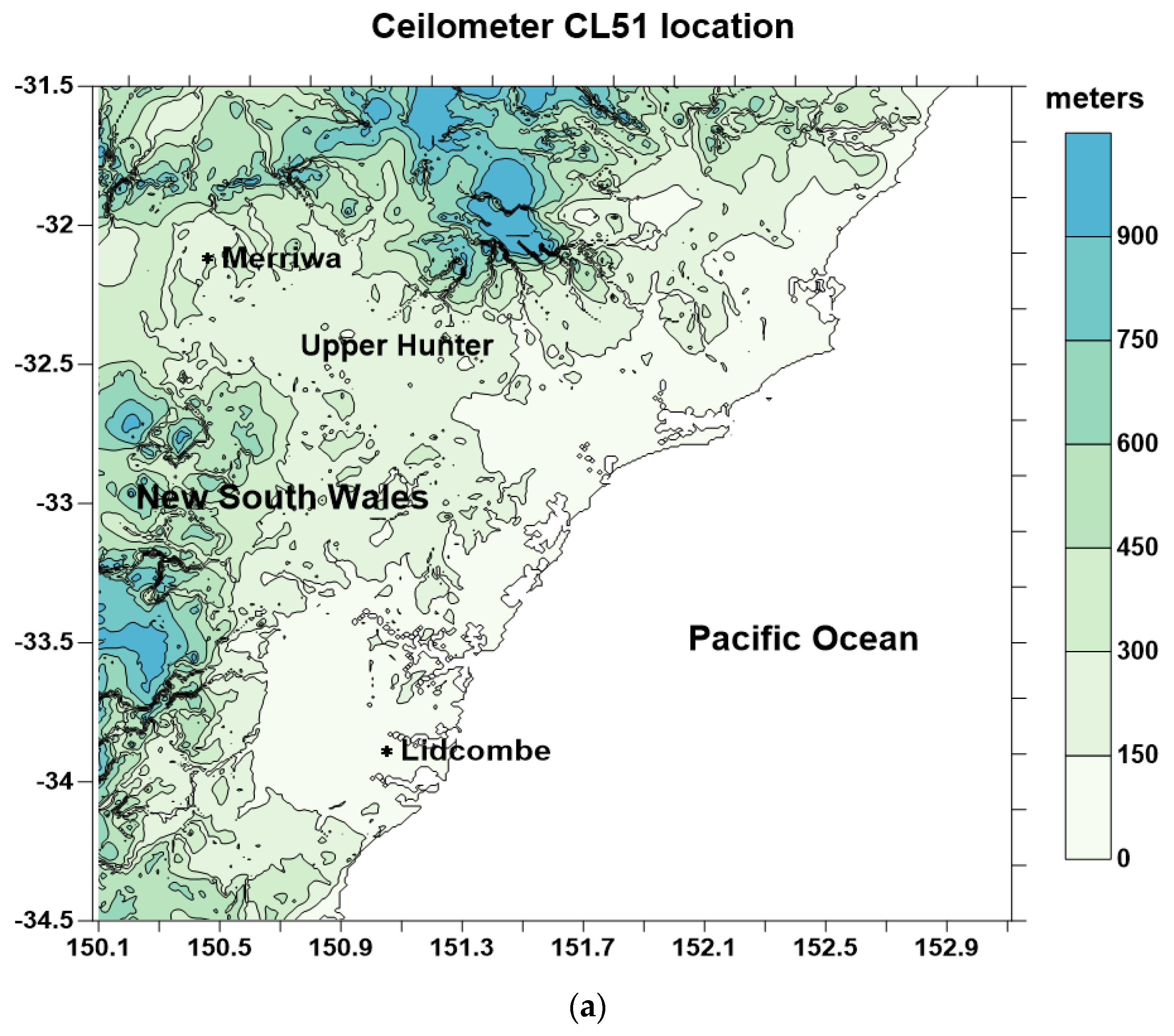
Currently, the Climate and Atmospheric Science (CAS) Branch of the NSW DPIE (New South Wales Department of Planning, Industry and Environment), Australia operates two Vaisala CL51 ceilometers located at Merriwa and Lidcombe sites. The Merriwa ceilometer near the Upper Hunter (northwest of Sydney) is used to detect the aerosol layers, including dust, transported from western NSW (Figure 1). The data collected from the two ceilometers were also used to assess and determine their suitability for calculating the mixing layer height time series continuously within the atmospheric planetary boundary layer (PBL). Vaisala has used the proprietary algorithm based on the Münkel and Roininen gradient method in the CL31 and CL51 ceilometers to derive the mixing height time series from the aerosol layer profiles, as measured by the ceilometers.

The main aim of this study is to apply the ceilometer measurements to three areas of interest in understanding air pollution process:

(1)

The relationship of air pollutant surface concentrations with MLH;

(2)

The evaluation of PBLH as simulated in air quality models over the modelling domain;

(3)

The dispersion and transport of air pollutants such as aerosols from emission sources to the atmosphere.

Accurate and continuous measurements of MLH are needed for relevant air quality assessments. Ceilometer technology can be used to retrieve the mixing height and to produce information on the vertical mixing and atmospheric structure over a selected area, as well as detecting cloud base and aerosol layers above ground. Results can be used to investigate the relationship between the evolution of the daytime mixed-layer height and air pollution under conditions where changes in concentration depend on the urban boundary-layer growth and air entrainment from the free atmosphere, the surface meteorology and the emission of air pollutants and precursors.

Air quality modelling and forecasting is important in air quality management. In this study, we used the derived MLH data from the two selected ceilometers to compare with the predicted PBLH from the NSW DPIE’s forecast and air quality models, CCAM-CTM (Conformal Cubic Atmospheric Model—Chemical Transport Model) and WRF-CMAQ (Weather Research Forecast—Community Multiscale Air Quality Modelling System). The data collected at the two selected ceilometer sites for the two periods in February 2021 and April 2021 were used to derive the corresponding MLH. In previous studies, Uzan et al. 2020 [12] have used MLH observed from ceilometers in Israel to validate two meteorological models, the European Centre for Medium-Range Weather Forecasts (ECMWF) Integrated Forecast System (IFS) global model and the Consortium for Small-scale Modeling (COSMO) regional model. Both of these models calculate the PBL height using the bulk Richardson number (Ri_b) method. They found the correlation of ceilometer MLH and PBLH predictions from the models, at a number of sites with varying height, terrain and distance from the coast, had the R values of 0.23 (Nevatim), 0.39 (Ramat David), 0.70 (Jerusalem), 0.72 (Weizmann), and 0.73 (Tel Aviv). The low correlation value of 0.23 at Nevatim was due to the complex terrain at this site, and thus the models found it difficult to simulate the PBLH properly.

The bulk Richardson number scheme is based on the simple ratio of convective turbulence (temperature) and mechanical turbulence (wind shear) and is represented by the bulk Richardson number formula:

$$R{i}_b=\frac{\left(\frac{g}{{\theta }_s}\right)\left({\theta }_z-{\theta }_s\right)\left(z-z_s\right)}{{(u_z-u_s)}^2+{\left(v_z-v_s\right)}^2}$$

(1)

where g is gravitational acceleration, θ is the potential temperature, z is at height z and s is first level height.

The PBLH is defined as the first height when the bulk Richardson number is greater than the critical value of ¼. The Ri_b is a simplified empirical form of the Richardson number, which is expressed as:

$$Ri=\frac{g}{T}\frac{\left(\delta \theta /\delta z\right)}{{\left(\delta u/\delta z\right)}^2}$$

(2)

Two most often used PBL schemes in WRF are the non-local first order closure YSU (Yonsei University) scheme, based on the bulk Richardson number, and the local second order closure MYJ scheme, based on solution of the turbulent kinetic energy (TKE) second-moment budget equation. The MYJ parameterisation scheme, based on the turbulence kinetic energy (TKE) budget equation, determined the boundary layer height as where the TKE decreases to a prescribed small value (0.2 m² s⁻²). The prognostic equation for TKE is solved by using diagnostic estimation of potential temperature, water vapor variance, and covariances [13]. Tyagi et al. 2018 [13], in their study of comparison of different PBL schemes in WRF with aircraft observation data, have shown that the local second-order closure TKE schemes perform better than the first-order closure schemes, such as the YSU scheme [13].

The validation of the NSW DPIE air quality models is important in having confidence in the forecasting ability and in scenario development of air quality model simulation for policy work. The PBLH is an important parameter in predicting air quality concentration and, as such, comparison with MLH lidar measurement data from the ceilometer is performed. The CCAM-CTM uses the bulk Richardson number to estimate the PBLH while the WRF-CMAQ is configured to use the TKE scheme for air quality forecasting at NSW DPIE.

Finally, besides using the ceilometer measurement to validate the PBLH estimate in air quality models, ceilometers can detect aerosol at various heights above a site, continuously, and hence they are useful to study aerosol transport. Coupled with the trajectory model, the transport from sources to the receptor site can be determined. The east coast of Australia frequently suffers high dust concentration from dust storm events originated in the Central Australia deserts and the western NSW dry lands, especially during drought conditions. The location of the ceilometer and a ground monitoring station at Merriwa, a remote site in the Upper Hunter region, can provide aerosol measurements on and above ground to study the dust transport from western NSW to the Upper and Lower Hunter regions of the Greater Metropolitan Region (GMR) of Sydney. The Upper Hunter is also an open-cut coal mining region. Therefore, dust from mining activities is also a concern of the people who live in the region. Mining dust can affect the ground measurement of aerosol concentration and the ceilometer measurement of aerosol layers above ground at Merriwa. We used the aerosol profile and MLH, as measured by the CL51 ceilometer, to study the aerosol transport from sources to the receptor site at Merriwa in some case studies, when high PM₁₀ concentration occurred at the site.

2. Data and Methods

2.1. Ceilometer Vaisala CL51 and Monitoring Data

The operation principle of the Vaisala CL 51 ceilometer is simple. Pulses of laser at 910 nm wavelength are emitted from the transmitter into the atmosphere. The scattered signals from scatterers (particles) are then received by the receiver. The signal is then range corrected (level 1), as the signal becomes weaker as the distance becomes larger. The range corrected signal (RCS) is obtained by multiplying the signal with r², where r is the distance. Data is processed to give profile data (level 2). The RCS is then used with the gradient minima method to detect the particle concentration boundaries. This is based on the observation that layered particles are confined in the boundary layer, above which there will be no lidar reflection. The boundary layer is then determined from the gradient method to find local minima, and the lowest of these gradient minima marks the top of the mixed layer.

Various gradient methods have been proposed [14,15]. The method proposed by [7] is implemented in Vaisala CL31 and CL51 BLView software to produce MLH data (level 3). Knepp et al. 2017 [5] evaluated the processing algorithm used in Vaisala CL31 and CL51 and the Structure of the Atmosphere (STRAT) algorithm as an open-source alternative to Vaisala BLView. They showed that much of the algorithm differences could be due to local meteorology impacts and precipitation events that pose algorithm difficulties. Otherwise, there was little difference between algorithms, especially at a time scale of 1-h resolution, as compared to a shorter time scale. Validation of the Vaisala method, by comparing MLH as derived from the ceilometer measurements with the observed radiosonde data, was performed at Sterling, VA, USA [7], Colorodo, USA [5], or with AMDAR (Aircraft Meteorological Data Relay) aviation data at Perth, WA, Australia [16]. The earliest studies, in 2008 and 2009 at Sterling, VA, USA [7], and Perth, WA, Australia [16], were conducted to evaluate the Münkel and Roininen gradient method as implemented in Vaisala CL31 to determine the PBLH from the lidar return signal. A large variety of ceilometer profiles under different meteorological conditions were compared to the sounding temperature profiles in Stirling and to the AMDAR data in Perth, which showed that the method can be applied for automatic boundary layer structure investigation. A later study in Colorado [5], using the algorithm as implemented in CL31 and CL51, showed that sonde-derived boundary layer heights were higher (10–15% at midday) than lidar-derived (CL51) mixed-layer heights.

The files from these processed levels (level 1 to level 3) in the CL31 and CL51 are stored in netCDF format. Most of the time, one needs to look only at the Level 3 data files which can be used with BL-View software, as provided with the instrument to determine the MLH using a built-in algorithm. The detection method works best on a clear-sky day. During a rain period where lots of echoes are received, even with filtering, the method struggles or does not work. The boundary layer scan resolution of CL51 is 10 m with a reporting interval of 36 s, and the range for a boundary layer fine structuring profile is 4000 m. The cloud base range is 13,000 m, as compared with 7500 m of the previous Vaisala CL31.

Recent non-propriety algorithm CABAM (Characterising the Atmospheric Boundary layer based on ALC Measurements) has been used by [17,18], and validated with AMDAR (Aircraft Meteorological Data Relay) measurements and applied to characterise the urban boundary layer over London. This is the first non-proprietary mixed layer height algorithm, specifically designed for the commonly deployed Vaisala CL31 ceilometer [17,18]. There are other public domain algorithms to determine the cloud height and MLH from lidar measurements. The Structure of the Atmosphere (STRAT v1.04) algorithm can determine cloud height and MLH from a variety of lidar instruments including the CL51. STRAT package is available as MATLAB and Python code and is a good alternative to BL-View from Vaisala [5,19]. The other publicly available algorithm is the UMBC algorithm, which was developed independently for estimating MLHs from lidar backscatter profiles using a covariance wavelet technique (CWT) similar to STRAT [5]. The ideal curve fitting (ICF) algorithm is another method to estimate the MLH from the lidar signal profile. This method was used by Peng et al. 2017 [20] using a CL51 lidar profile in their study of PBLH in Shanghai, China.

The MLH, as derived by the Münkel and Roininen method [7] and provided by Vaisala CL51, was extracted from Level 3 and used in this study. Meteorological and air quality data at the ceilometer sites were obtained from the DPIE air quality monitoring network, which covers most of New South Wales.

2.2. Study Area

Figure 1a shows the location of the two Vaisala CL51 ceilometers in New South Wales. Merriwa is located in the Upper Hunter Region of NSW, and known as one of the most fertile farming areas in the country. Dust pollution has been recognised as a major type of pollution occurring in the area. An air quality monitoring station located on the Merriwa Scone Road was established in 2012, as a background site for fine particle PM₁₀ measurements. The geographic coordinate of the station is −32.12° latitude and 150.46° longitude.

Lidcombe ceilometer is co-located at the DPIE Lidcombe air quality monitoring station site situated in the centre of a metropolitan area of Sydney (−33.88° latitude, 151.05° longitude). The location is ideal to observe the aerosol layers and PBL above the urban areas and the other ground-based meteorological and air quality variables, such as wind speed, temperature, Ozone, PM₁₀, PM_2.5 and other pollutants.

Topography and meteorological conditions influence the evolution of mixing height profiles and the associated atmospheric stability classes. Selected available meteorological parameters, such as wind speed and wind direction, surface temperature, and humidity were selected to study their effects on mixing height at Merriwa and Lidcombe. The time series of selected parameters were plotted against the corresponding mixing heights and the obtained results are presented in following section.

2.3. Air Quality Model Validation Using Ceilometer Measurement

Currently, DPIE uses two air quality models for forecasting daily air pollution and policy scenario development: the CCAM-CTM (Conformal Cubic Atmospheric Model—Chemical Transport Model) model developed by CSIRO [21,22,23] and the State-of-the-Science WRF-CMAQ (Weather Research Forecast—Community Multiscale Air Quality Modeling System) model developed by US-EPA. In this study, we will use the derived PBL profiles from the ceilometer measurements at the Merriwa and Lidcombe sites to validate the predictions from each of the air quality models above. The results of the validation are presented in the following Results Section.

The simulation domain configuration, as shown in Figure 1b, for the WRF-CMAQ run was a three-nested domain with the outer domain (d01) covering much of Eastern Australia at the resolution of 12 × 12 km. The inner domain (d02) was at 4 km × 4 km resolution covering most of NSW, while the innermost domain (d03) was at 1 × 1 km resolution and covered the Greater Metropolitan Region (GMR) of Sydney [24]. The initial and boundary conditions and host data for meteorology were from the US National Centre for Environmental Prediction (NCEP) Final Reanalysis data. The physics schemes used in WRF are listed in

Table 1. WRF physics parametrisation.

Physical Parametrisation	Namelist Variable	Option	Model/Scheme
Microphysics	mp_physics	10	Morrison 2-moment Scheme
Land surface	sf_surface_physics	2	Unified Noah Land-Surface Model
Surface layer physics	sf_sfclay_physics	2	Eta Similarity Scheme
Planetary Boundary Layer	bl_pbl_physics	2	Mellor–Yamada–Janjic Scheme (MYJ)
Shortwave radiation	ra_sw_physics	4	Rapid Radiative Transfer Model for GCM (RRTMG)
Long wave radiation	ra_lw_physics	4	Rapid Radiative Transfer Model for GCM (RRTMG)
Cloud cumulus	cu_physics	5	Grell 3D Ensemble Scheme
Urban surface	sf_urban_physics	1	Urban Canopy Model

.

CCAM-CTM domain configuration as currently used in the DPIE forecast operation is shown in Figure 2. The host meteorological data for CCAM downscaling is provided by the Bureau of Meteorology (BOM) ACCESS-R (Australian Community Climate and Earth-System Simulator—Regional product). The CCAM physics options are listed as follows in

Table 2. CCAM physics parametrisation.

Physical Parametrisation	Scheme
Topography/Land use	MODIS satellite data
Data assimilation	Scale-selective filter to nudge towards the ACCESS-R data
Micro-physics	Prognostic condensate scheme
Longwave and shortwave radiation	GFDL (Geophysical Fluid Dynamics Laboratory) scheme
Land surface	Kowalczyk scheme
Planetary boundary layer	Local Richardson number and non-local stability
Urban canopy	Town Energy budget approach

, and used in previous work [24,25].

The 2 periods of validation were 12 to 19 February 2021 (austral summer) and 20 April 2021 to 2 May 2021 (austral autumn). The predictions of PBLH from the models were compared with CL51 lidar measurements for those periods. In CCAM, the bulk Richardson number (Ri_b) method was used to estimate the PBLH, while for WRF, the PBLH was estimated by using the Mellor–Yamada–Janjic local scheme (MYJ) [26,27,28] as a configuration option in our study. For the period of 12 to 19 February 2021, at Merriwa, there were no clear sky days, 3 partly clear days, 1 mostly cloudy day and 4 cloudy days. The ratio was 0% clear days, 50% partly clear and 50% cloudy. While at Lidcombe, the ratio was 0% clear days, 50% partly clear and mostly cloudy, 50% cloudy. For the autumn period of 20 April to 2 May 2021, at Merriwa the ratio was 75% clear days, 25% partly clear days. At Lidcombe, the ratio was 42% clear days, 50% partly clear and 8% cloudy days.

Table 3. Cloud status at Lidcombe and Merriwa during the austral summer period (12 to 19 February 2021) and austral autumn period (20 April to 2 May 2021).

	Lidcombe		Merriwa
	Summer Period	Autumn Period	Summer Period	Autumn Period
Clear sky days	0 (0%)	5 (42%)	0 (0%)	9 (75%)
Partly clear days	1 (12.5%)	6 (50%)	3 (37.5%)	3 (25%)
Mostly cloudy days	3 (37.5%)	0 (0%)	1 (12.5%)	0 (0%)
Cloudy days	4 (50%)	1 (8%)	4 (50%)	0 (0%)

summarises the cloud status at the 2 sites for the 2 periods under consideration.

2.4. Application of Ceilometer Measurement to Study the Transport and Sources of Aerosols at Merriwa

Merriwa is a remote site in the Upper Hunter where dust sources from western NSW or mining activities in this region can cause high dust events occurring in the Lower Hunter of the Greater Metropolitan Region (GMR) of Sydney. To determine which source—either dust from a dust storm in western NSW, or dust from mining activities, causing high ground PM₁₀ concentration as measured at the Merriwa monitoring station—a back trajectory model was used in this study. The trajectory model used in this study was the HYSPLIT Lagrangian backward trajectory model from NOAA.

3. Results and Discussion

3.1. Relation of Ceilometer PBLH with Surface Meteorological Variables and Air Pollutant Concentration

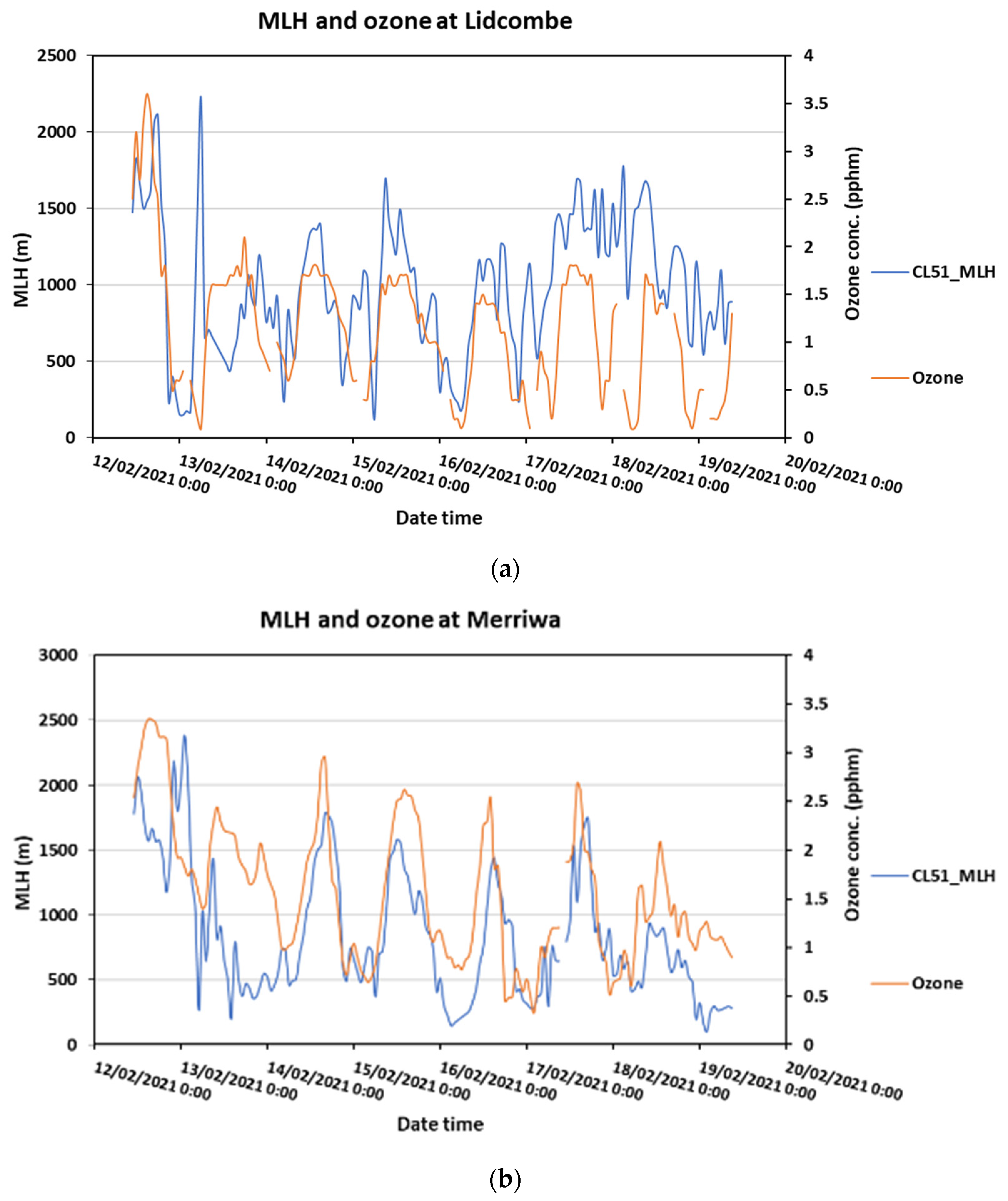
The influence of selected meteorological conditions on the derived ML profiles from the ceilometer measurements was studied using the data for the period starting 12 February 2021 to 19 February 2021.

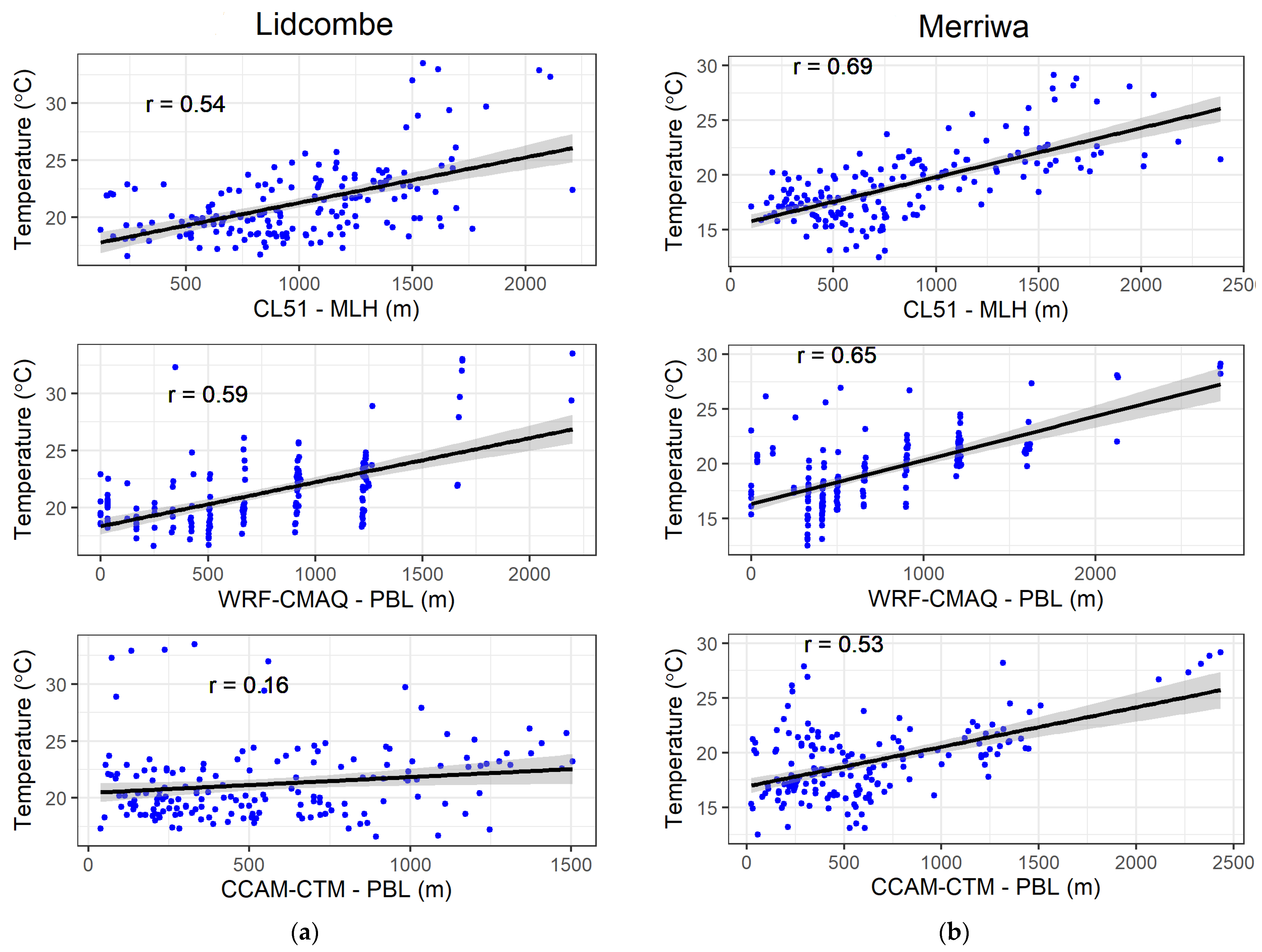
The selected meteorological variables from the DPIE Lidcombe monitoring station showed that temperature and solar radiation were strongly correlated with MLH, as shown in Figure 3 and Figure 4. This was expected as, during daytime, the growth of the ML is mainly driven by thermal convection.

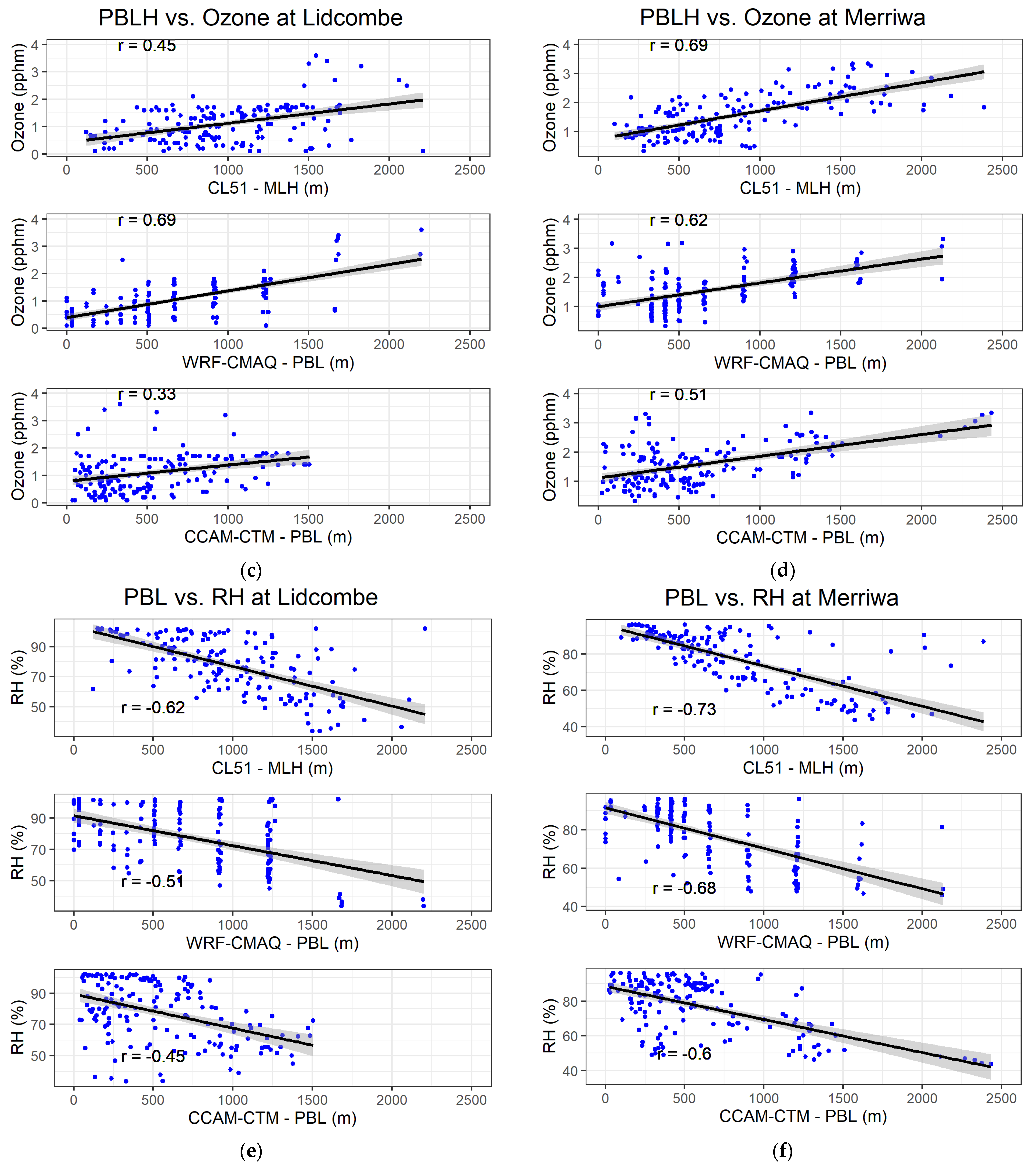
In comparison with relative humidity (RH), the PBL measurements from the ceilometer were negatively correlated with RH (Figure 4e,f). The result was consistent with a study by Dang et al. 2016 [29] at Lanzhou, a semi-arid area in northwest China where they found the MLH as measured by a Micro-Pulse Lidar instrument (MPL-4, Sigma Space) was negatively correlated with relative humidity. Allabakash and Sanghun 2020 [30], in their study of climatology of PBLH-controlling meteorological parameters, have also shown that RH was negatively correlated with PBLH over Korea. Australia is a dry continent; high temperature is usually associated with low RH. When temperature is low and the RH is high, the sensible heat flux will be reduced, and hence the ML growth is slower. The inverse relation between temperature with relative humidity explains the MLH is positively correlated with temperature, but negatively correlated with RH.

For Merriwa, the results are similar to those observed at Lidcombe in terms of correlation of MLH with temperature, solar radiation, and relative humidity.

The derived ML profiles from CL51 lidar were also used to examine the relationship with the ozone profiles. This comparison, as illustrated in Figure 4, shows a strong correlation between ozone and ML height. The increase in the MLH is associated with the increase in temperature. It is known that, during daytime, the temperature increases will result in a higher photochemical reaction rate and higher ozone production, even though the MLH increase also reduces the ground ozone level due to vertical mixing. For this analysis period from 12 February 2021 to 19 February 2021, the photochemical rate production was higher than the dilution factor from the vertical mixing process.

For other pollutants, such as PM₁₀, PM_2.5, NO₂, the relations between each of these pollutants at ground level and MLH for the austral summer period 12 to 19 February 2021 at the two sites were not clear, and changed with the location, with a correlation coefficient R of 0.23, −0.01 and −0.04, respectively, at Lidcombe, and 0.44, 0.08, −0.11 at Merriwa. For PM₁₀, positive correlation with MLH was stronger at the Merriwa rural site as compared to that at the Lidcombe urban site. Dust from inland NSW could have played a role at the Merriwa site, while fine particle PM_2.5 had no correlation with PBLH at both sites. The scattered plots and correlation for O₃, PM₁₀, PM_2.5, NO₂ and NO_x at Lidcombe and Merriwa for the periods of 12 to 19 February 2021 and 20 April 2021 to 2 May 2021 are provided in the Supplementary Materials.

During the austral autumn period (17 April to 2 May 2021), the positive correlation of PBLH and O₃ were 0.73 at Lidcombe and 0.03 at Merriwa. It is clear that O₃ increased with increasing PBLH at the Lidcombe urban site for the two periods considered, but not at the Merriwa rural site. For PM₁₀, PM_2.5, NO₂ and NO_x, during the autumn period, the correlation coefficients were −0.22, −0.23, −0.54, −0.53 at Lidcombe, and −0.01, −0.24, −0.12, −0.18 at Merriwa. For PM₁₀ and PM_2.5, the correlation coefficients were negatively small, showing practically little relation between these pollutants at ground level and MLH. Negative correlation between PBLH and NO₂ (and NO_x) concentration was stronger at the urban Lidcombe site than that at Merriwa, and NO_x concentration was also much higher at Lidcombe. This negative correlation was mirrored with the ozone and PBLH positive correlation. Photochemical reactions probably played an important role in the NO_x, O₃ and PBLH relations.

In a study of the impact of mixing layer height on air quality in winter in Delhi, India, Murphy et al. 2020 [31] analysed CL51 ceilometer MLH data and ground monitoring data. They found the ozone was strongly correlated with MLH, but PM_2.5 had less correlation with MLH. Our results, however, are more consistent with Geiß et al. 2017 [32] in their study on the relations between MLH from CL51 and ambient pollutant concentration measured on a ground station in Berlin. Their results showed that the correlations between MLH and concentrations of pollutants (PM₁₀, O₃ and NO_x) for different locations in Berlin were varied. There was no clear pattern in correlation with PM₁₀, which was quite different for different sites, whereas the correlation with NO_x seemed to depend on the vicinity of emission sources on main roads [32]. Only in the case of ozone, a clear positive correlation was found with R of 0.69 at Merriwa and 0.45 at Lidcombe, from 12 to 19 February 2021 (summer) and 0.73 at Lidcombe, and 17 April to 2 May 2021 (autumn). This is not surprising, as ozone is a secondary pollutant formed from photochemical processes driven by sunlight occurring over a regional scale, and hence it has a longer correlation distance than other pollutants [33].

3.2. Ceilometer MLH and Model Forecast PBL Comparisons

Comparison of MLH, as measured at Merriwa, and the predicted PBLHs from CCAM-CTM and WRF-CMAQ for the period 12 to 19 February 2021 and 20 April 2021 to 3 May 2021, based on performance metrics of mean bias (MB), normalised mean bias (NMB), root mean square error (RMSE), correlation coefficient (r) and index of agreement (IOA), is summarised in

Table 4. Performance metrics of PBLH prediction (in metres) by WRF and CCAM, as compared to CL51 observation.

WRF-CMAQ vs. CL51
Site	n 1	MB 2	NMB 3	RMSE 4	r 5	IOA 6
Lidcombe	417	−158	−0.20	613	0.43	0.51
Merriwa	371	−140	−0.19	497	0.58	0.56
CCAM-CTM vs. CL51
Lidcombe	417	−312	−0.40	647	0.31	0.47
Merriwa	371	−244	−0.33	580	0.41	0.47

¹ Total number of hourly values during 12 to 19 February 2021 and 20 April 2021 to 2 May 2021; ² mean bias; ³ normalised mean bias; ⁴ root mean square error; ⁵ Pearson correlation coefficient; ⁶ Index of Agreement. Units of MB and RMSE are in metres.

. Overall, both models underpredicted the PBLH (MB is negative) and the PBLH as predicted by WRF performed slightly better than CCAM at both sites. The model prediction at Merriwa was better that that at Lidcombe.

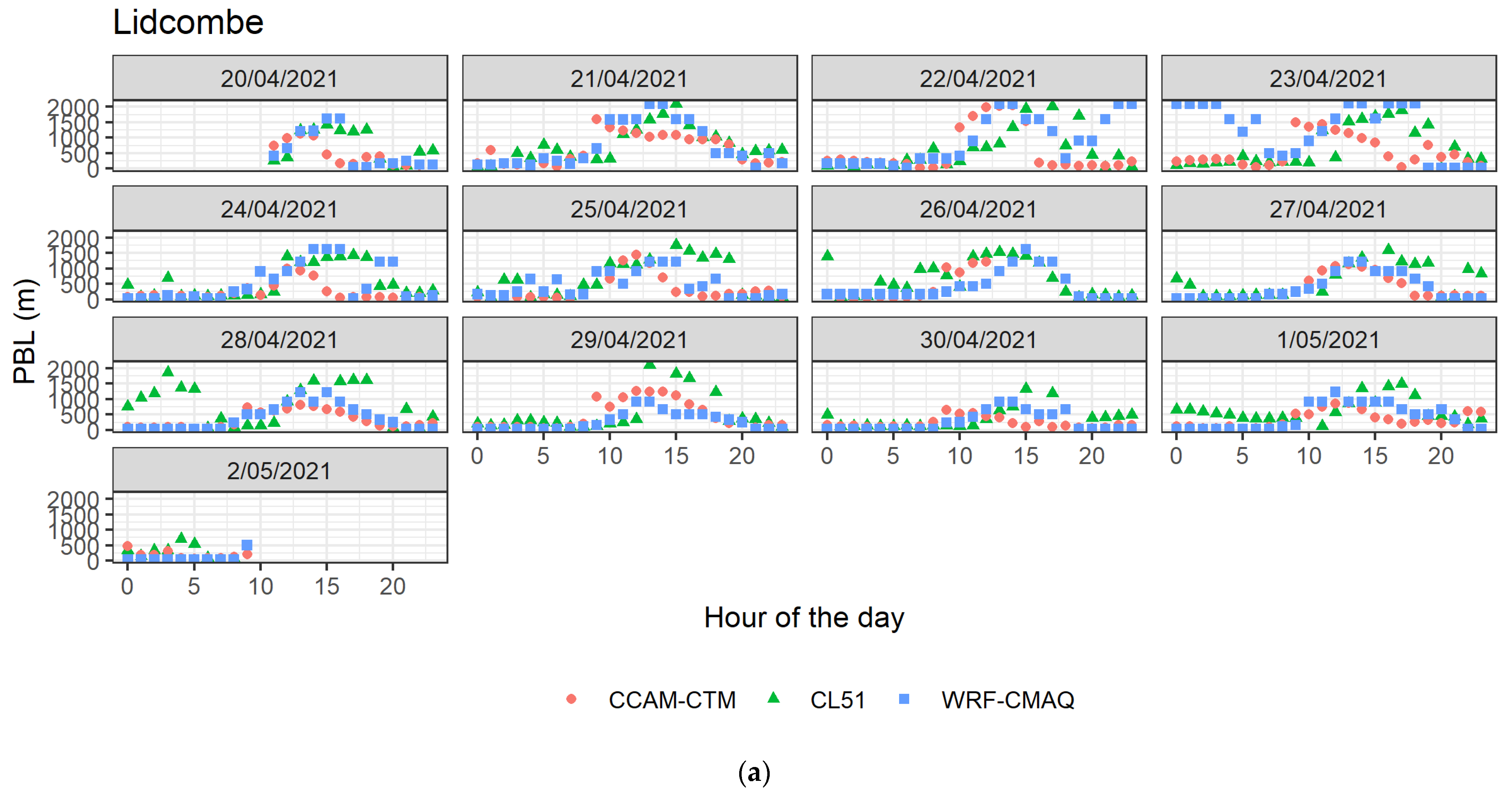
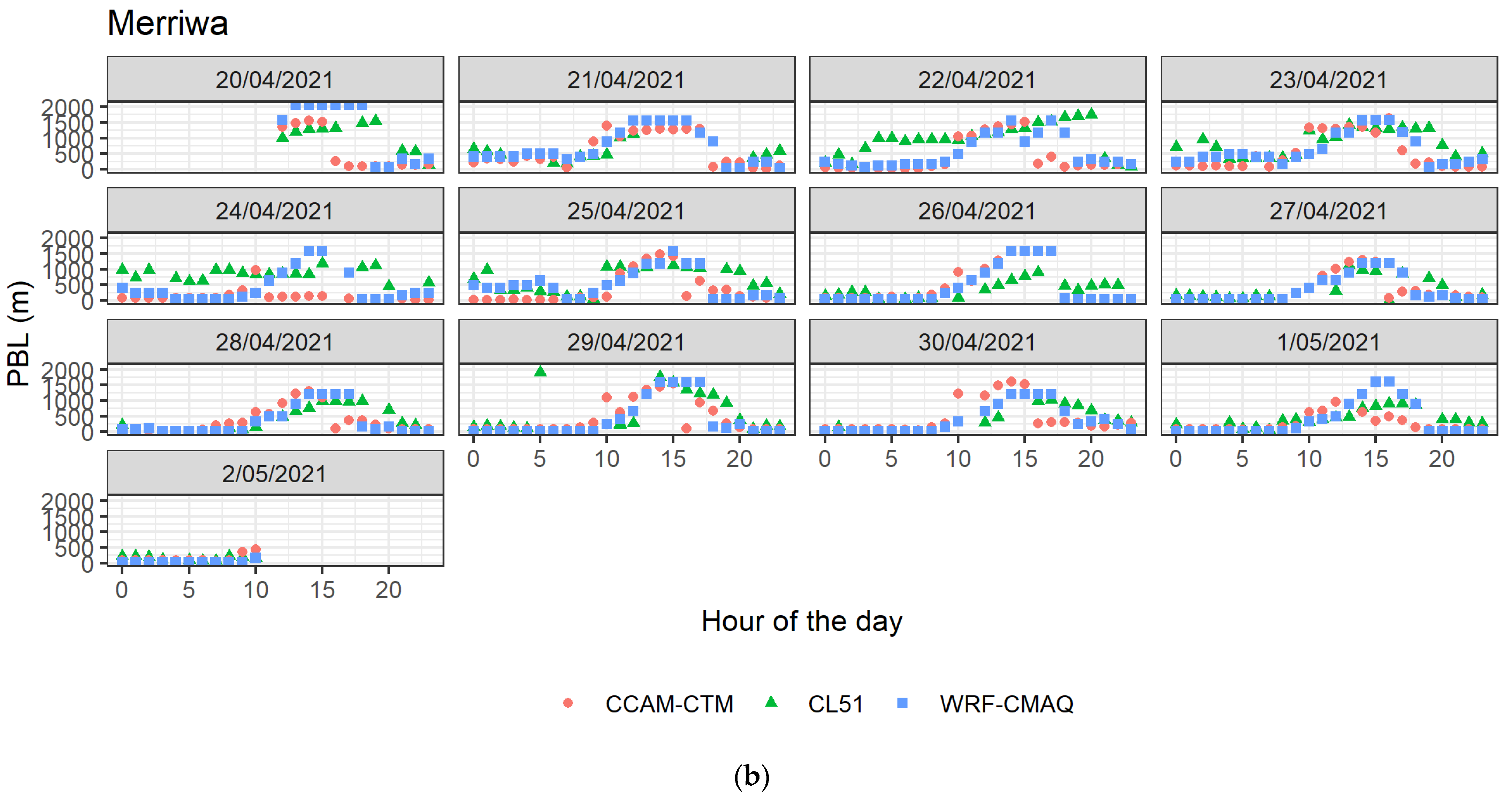
Another comparison analysis was also performed for an autumn period from 20 April 2021 to 3 May 2021. The time series of the predicted PBL profiles by the selected numerical models and the derived MLH from the ceilometers, during the period from 20 April 2021 to 2 May 2021, are shown in Figure 5. There is a reasonable agreement between the models and the observation. At Lidcombe, the peak of the MLH occurred at around midday from 12:00 to 15:00 h, as expected, usually at the height from 1500 to 2000 metres. Both CCAM-CTM and WRF-CMAQ slightly underpredicted the MLH peaks. The model predictions of the nocturnal PBL heights were lower than the observations highlighting the complex structure of this layer during this period. Shi et al. 2020 [4] also reported the nocturnal boundary layer heights were seriously underestimated by the WRF model in a study in Beijing from 26 to 31 December 2017.

At Merriwa, when compared to ceilometer observations for the period between 20 April 2021 to 2 May 2021, both the air quality models CCAM-CTM and WRF-CMAQ predicted the PBLH reasonably well. Similar to the Lidcombe site, the nocturnal PBLH predictions were underpredicted. In particular, on the 23 and 24 April 2021, the estimated nocturnal MLH was high, at mostly above 500 m, indicating warmer air above ground. However, the prediction of CCAM-CTM PBLH was less than 100 m, while WRF-CMAQ nocturnal PBLHs varied between 50 m to 400 m on 23 April 2021, and were reasonably good compared to observation. Similarly, WRF-CMAQ nocturnal PBLHs on 24 April 2021 varied between 50 to 600 m. The underprediction of nocturnal PBLH in the two air quality models can also be due to MLH being assigned erroneously to the residual layer height, rather than the minimum height in the stable layer below it in the minimum gradient detection algorithm used in the CL51 ceilometer [32].

Compared to Lidcombe, the CL51 MLH measurements for this summer period showed the maximum MLH at about 1500 m, compared to 1500–2000 m at Lidcombe during daytime convection condition.

Overall, the performance of the WRF-CMAQ and CCAM-CTM, as currently configured and used for forecasting, in PBLH prediction when compared to the CL51 MLH observation, was reasonably good—based on the performance indicators presented above. The results for CCAM are consistent with the CCAM vertical wind and temperature prediction in the previous study [34]. The differences in the PBLH prediction between WR-CMAQ and CCAM-CTM could also be due to the different meteorological host data (NCEP FNL and ACCESS-R) used, and the boundary height calculation schemes—Mellor–Yamada–Janjic Scheme (MYJ) in WRF, and bulk Richardson number scheme in CCAM.

The bulk Richardson number scheme was also implemented in the YSU (Yonsei University) non-local scheme in WRF. The PBLH calculation in the MYJ scheme in WRF was based on TKE (turbulent kinetic energy) parametrisation, while the ceilometer MLH was derived from the aerosol backscatter profile minimum gradient.

Scarino et al., 2013, [35] compared the WRF-simulated PBLH based on the MYJ scheme with MLH data derived from an airborne high spectral resolution lidar (HSRL) along the flight paths. The HSRL was deployed to California onboard the NASA LaRC B-200 aircraft in May and June 2010. The ML or daytime CBL determination from the airborne lidar was based on a Haar wavelet transform with multiple wavelet dilations to identify the sharp gradients in the aerosol backscatter profiles located at the top of the boundary layer. They found reasonable agreement between the WRF-Chem predicted PBLH and the observed HSRL ML height with a correlation (r) of 0.58, a mean bias of −157 m, and an RMS of 604 m during the Los Angeles May 2010 campaign. The same comparison for the Sacramento campaign in June 2010 showed a correlation of 0.59 (r value), a mean bias difference of 220 m, and RMS of 689 m. These values are comparable to our results shown in Table 4. The chemistry option in their WRF-Chem was based on the Regional Acid Deposition Model, version 2 (RADM2) and the Modal Aerosol Dynamics Model for Europe/Secondary Organic Aerosol Model (MADE/SORGAM) as the aerosol module.

Scarino et al., 2013, [35] also compared the PBLH, as derived from vertical aerosol profile prediction from WRF-Chem using the same wavelet transform on profile data as used in the HSRL back scatter data, with HSRL ML height data. Reasonable agreement was also obtained. For example, with the Sacramento campaign dataset, the correlation between the WRF-Chem and the HSRL ML heights across all flights was 0.6 (r value), with a mean bias difference of 194 m, and an RMS difference (or error) of 586 m.

The above comparison results using two different methods of calculating the MLH and PBLH (one using potential temperature and one using aerosol backscatter) is very similar. This result from their study has important implications: it means that PBLHs determined using temperature profile and those using aerosol profile are equivalent. The PBLH prediction in WRF-Chem using the MYJ scheme based on turbulent kinetic energy parametrisation gives similar result to that based on the aerosol profile peak gradient method, such as the Haar wavelet transform.

Milovac et al., 2015 [36], in their study of comparing different boundary layer schemes and land surface models (LSMs) used in WRF in Germany, found that the land surface processes can have an impact not only on the lower CBL, but also extend up to the interfacial layer and the lower troposphere. Using six different PBL and LSM schemes (including the MSY PBL scheme and the Noah land surface model, as used in our study), the impact of diurnal change in the humidity profiles was more significant at the interfacial layer than close to the land surface. They concluded that the representation of land surface processes has a significant impact on the simulation of mixing properties within the CBL.

Other uncertainties include the detection algorithm and MLH gradient method used in processing the lidar echo signals from ceilometers. For example, Bedoya-Velásquez et al. 2021 [37] have recently improved the range-corrected signal (RCS) affected by water vapor absorption, as it was found that raw ceilometer signal overestimates the water vapor-corrected one, mainly below 1 km AGL. If vertical water vapor data is not available, then relative humidity data profiles can be obtained from the GDAS (Global Data Assimilation System) database to correct the RCS. As Geiß et al., 2017, [32] have pointed out, the MLH as determined from the layer aerosol profile can give an error, as the residual layer is misinterpreted as the mixing layer during night-time.

Ceilometer data signal processing and PBL analysis can be enhanced using layer information from MERRA-2 (Modern-Era Retrospective analysis for Research and Applications, version 2) such as vertical aerosol concentration from which lidar optical parameters, such as aerosol extinction and backscattering coefficients, can be calculated.

3.3. Aerosol Layer Structure and Aerosols Transport—Case Studies at Merriwa

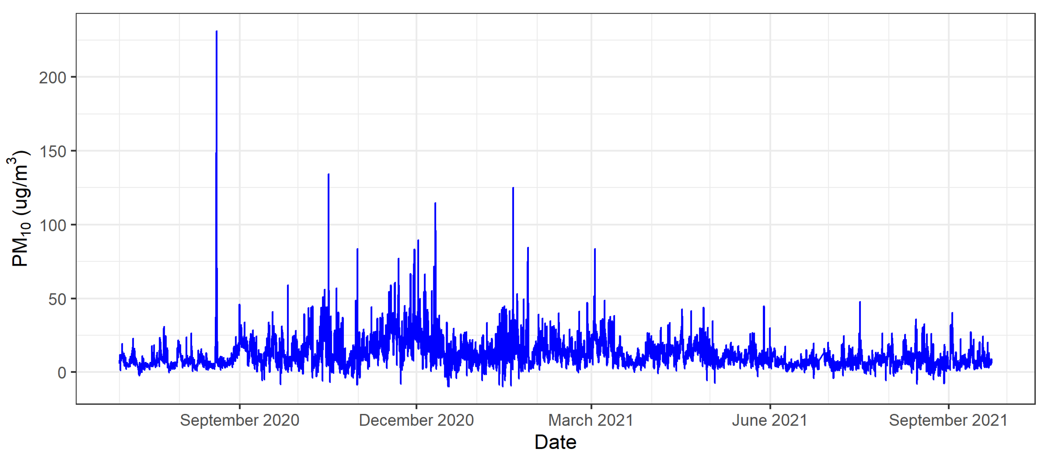
The Merriwa ceilometer has been installed and operational since 16 September 2020 at a remote rural site, west of the major towns in the Upper Hunter area, where dust from inland desert and from open-cut coal mining activities are the main sources. It is, therefore, of interest to find whether the ceilometer data at Merriwa can be used during high particle concentration events at this site, to track down whether the aerosols transported to the Upper Hunter region come from the inland desert natural source, or from within the coal mining activities that have caused concerns to the people living in the region. Since its operation in September 2020, the measurement and its performance in determining the ML height and cloud base height at various hours of the day provided us with an understanding of the evolution of the ML above ground. The following case study analysis of some PM₁₀ event days at Merriwa illustrates the use of ceilometer data to understand and interpretate the source and cause of these high PM₁₀ concentration, as measured at the Merriwa monitoring station.

The concentrations of PM₁₀ measured at the Merriwa monitoring site from 1 July 2020 to 22 September 2021 are shown in Figure 6. The time series of concentrations show no high PM₁₀ events after 12 March 2021 (the date when the Merriwa ceilometer was put in operation). However, there were occasional spikes for a few hours with lower levels. Before March 2021, there were a few particle events with a major dust storm on 20 August 2020 (large spike above 250 μg/m³ in Figure 6). Other smaller particle events happened on 16 October 2020, 10 December 2020 and 19 January 2021.

It is anticipated that dust events could happen in the coming months during spring and summer 2021–2022, and the ceilometer will provide informative measurements to detect the dust plumes. Similar to the study [10] of dust detection, using lidars and ceilometers from volcanic ashes, with case studies of event days where high ground-level PM₁₀ concentrations occurred, in the present analysis we also analyse the three particle events on 16 October 2020, 10 December 2020 and 19 January 2021 at Merriwa to determine where the sources, and the causes of these events at the receptor, are. These three case studies show the influence of meteorology on the transport of emitted aerosols from various sources to the receptor site and the complexity of meteorological processes in understanding the pattern of aerosol profiles at the receptor site.

The CL51 ceilometer at Merriwa has the profile measurements for those event days which are analysed in detail as described below, with corroboration from satellite data and back trajectory analysis.

3.3.1. Event Day 16 October 2020

The 16 October 2020 ceilometer measurement is shown in Figure 7. The peak PM₁₀ concentration was detected at 18:00 AEST. This day was cloudy as detected by satellite MODIS Terra/Aqua above Merriwa. The thick foggy water droplet from 5 am to 9 am was close to the ground on the morning of 17 October 2021, as seen in Figure 7. On 16 October 2020, the MLH as measured by the ceilometer dropped from ~2000 m to ~500 m at 18:00 AEST. This corresponded to the high PM₁₀ concentration measured at the Merriwa monitoring station. Back trajectory analysis for 48 h was performed to determine the source of this high PM₁₀ concentration detected at Merriwa.

Figure 8 shows the source of this high PM₁₀ concentration from the north west and north of Merriwa, with satellite data showing high AOD in this area. The HYSPLIT back trajectory analysis was run at 10 m, 20 m and 50 m above ground level (AGL) with GDAS (Global Data Assimilation System) 1° resolution data from NOAA.

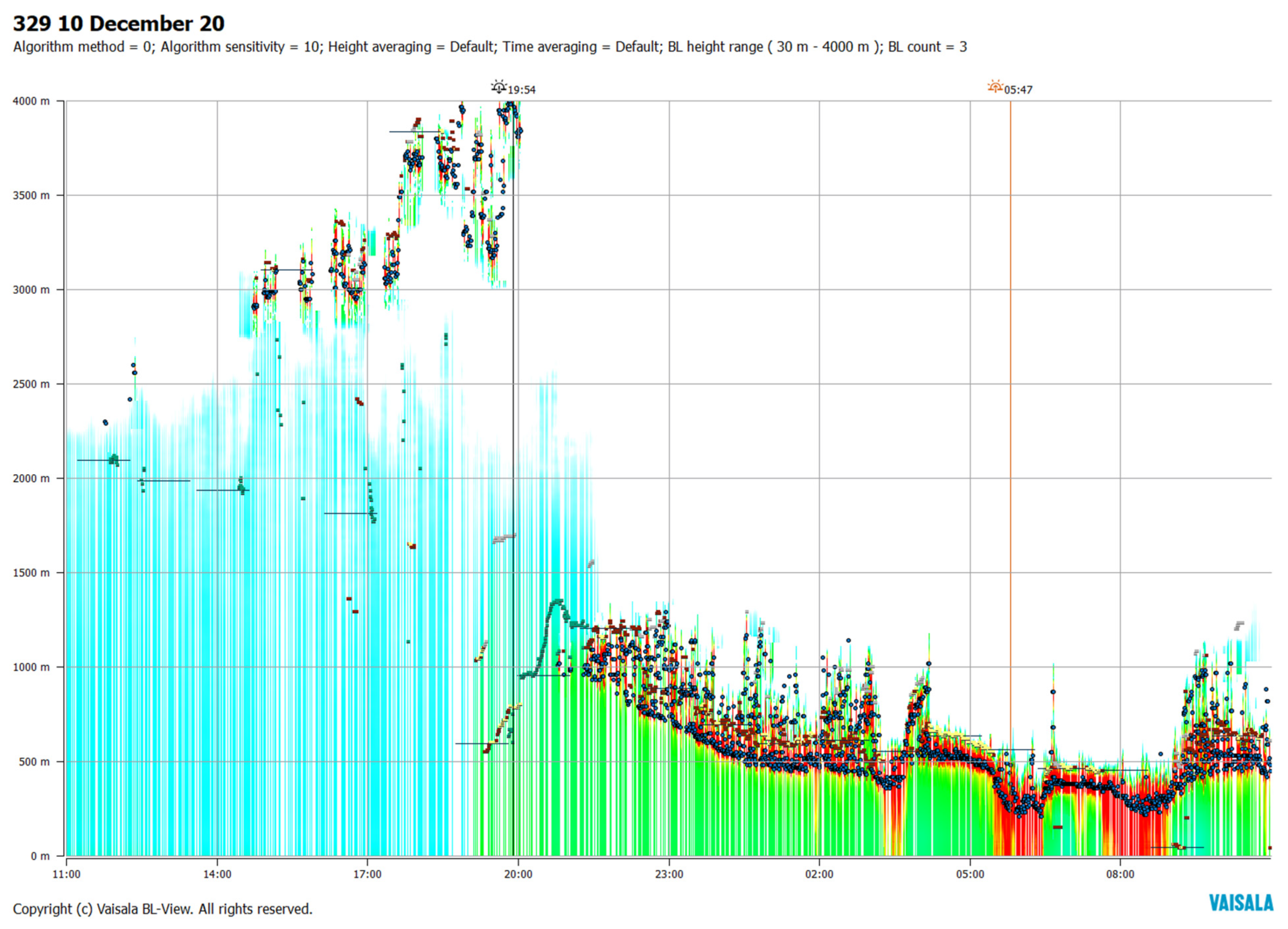
3.3.2. Event Day 10 December 2020

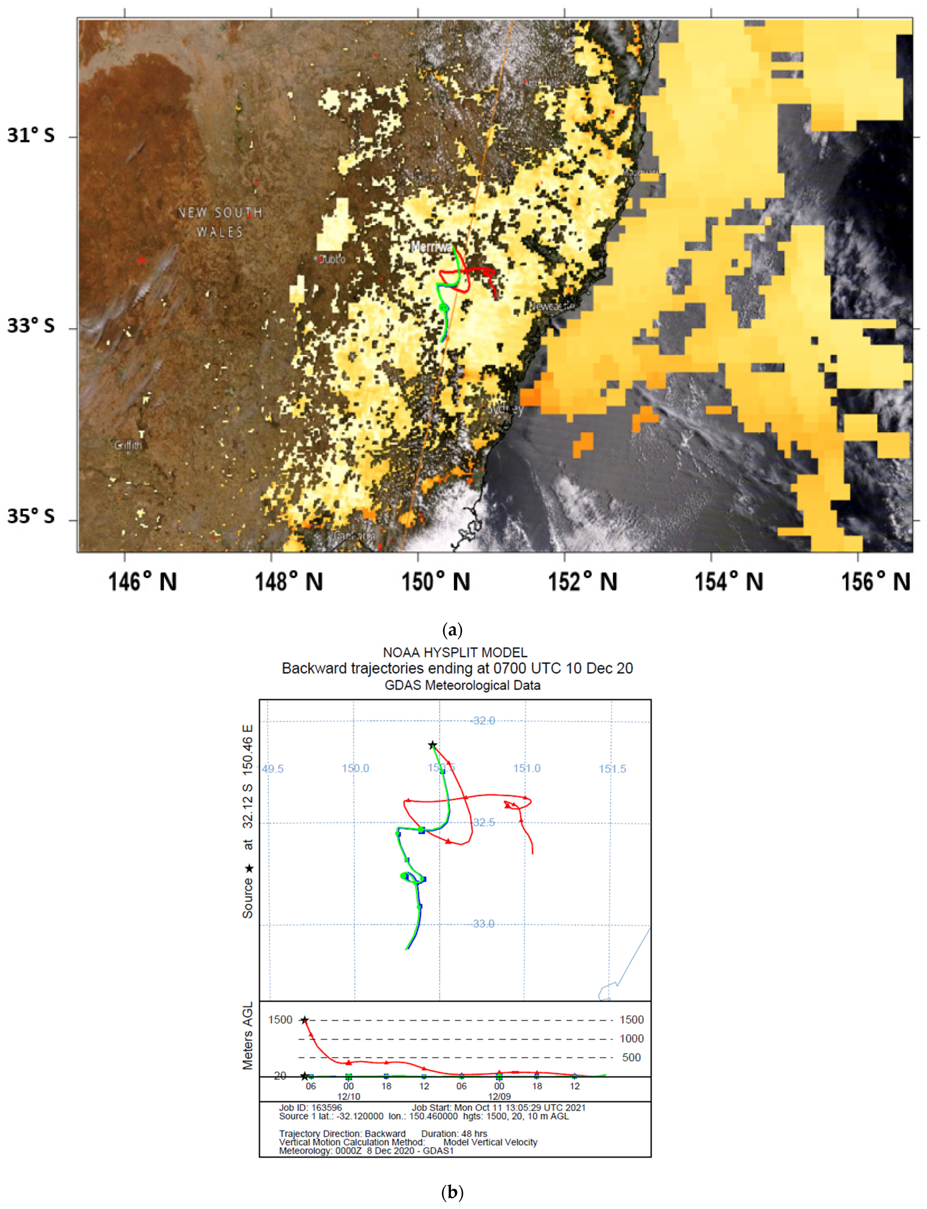
For the 10 December 2020, high PM₁₀ occurred at 17:00 AEST. Similar to the above analysis, back trajectory analysis was performed and ceilometer data on this day is shown in Figure 9. The MLH increased after 17:00 AEST and only decreased about 3 h later. This shows that the vertical profile of atmospheric structure had no influence on the high peak ground level concentration at Merriwa. The advection transport of aerosols was the main cause. This is confirmed by HYSPLIT back trajectory analysis.

The source of air parcels at 1500 m above ground level at Merriwa came from ground level (10 m) west of Newcastle 48 h before, as shown by the ‘red’ trajectory in Figure 10. Air parcels at 10 m and 20 m AGL at Merriwa came from ground level air parcels north west of Sydney, as shown by the ‘green’ and ‘blue’ trajectories. There was no change in level heights of these trajectories during the 48 h transport of aerosols from the north west of Sydney, passing through the Upper Hunter, before reaching the Merriwa receptor. In other words, the horizontal advection transport of aerosols, which was emitted along the trajectory path and carried by the wind to the Merriwa receptor, caused the high PM₁₀ concentration at 17:00 AEST on 10 December 2020.

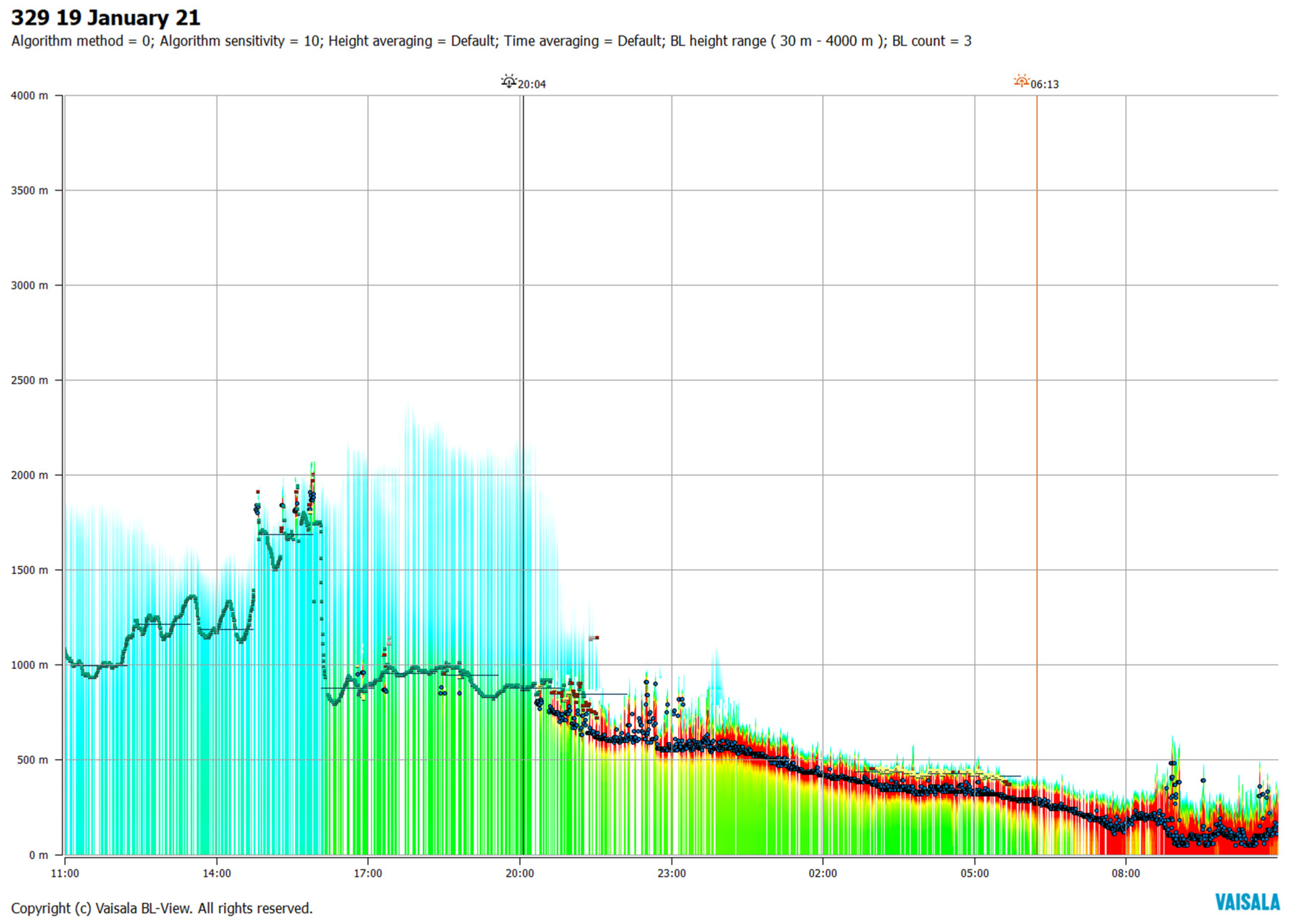
3.3.3. Event Day 19 January 2021

For the high PM₁₀ day of 19 January 2021 at 15:00 AEST, HYSPLIT back trajectory analysis at 10 m, 20 m and 50 m above ground level at Merriwa indicated that the source of the aerosols came from the south east and south. There was no cloud above Merriwa and the rest of NSW on this day, except in the Greater Sydney Metropolitan near the coast.

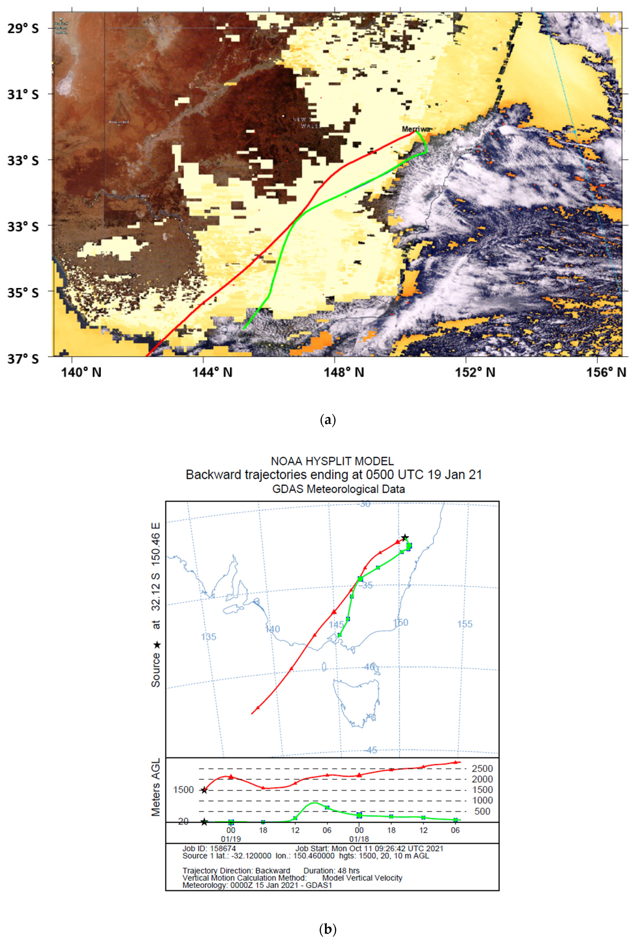
The ceilometer data at Merriwa on this day showed MLH was reduced from about 1500 m to less than 1000 m at about 16:00 AEST (Figure 11). The paths of the back-trajectory analysis at 10, 20 and 50 m AGL were at similar levels when passing over the Upper Hunter before reaching Merriwa. While at 1500 m AGL at Merriwa, the source of air parcels came from the south west and travelled at height above 1500 m, as shown in Figure 12.

From the three case studies above, it has been shown that the transport of aerosols to the Merriwa receptor can be from western or northern NSW (16 October 2020), but can also be from the south east in the Upper Hunter, or southern NSW (10 December 2020 and 19 January 2021). Dust is most likely from western and northern NSW, while anthropogenic sources are most likely from the south east in the Hunter region and from the southern NSW. Meteorology plays an important role in the transport of particles from natural sources or anthropogenic sources to the receptor point.

For future study, space-born lidar data from the CALIPSO satellite can be used to supplement information on aerosol vertical structure above Merriwa and Lidcombe. Even if there was missing ceilometer data, such as on 20 August 2020, the CALIOP lidar sensor onboard the CALIPSO satellite can provide some information on vertical structure above and near the Merriwa region on a day when the satellite passed over the region. For the high PM₁₀ events that occurred, ceilometer data and CALIPSO data can be used together to corroborate the measurement results. Li et al. 2021 [38], in their study on using the Lufft CHM15K ceilometer for retrieval aerosol characteristics including AOD, have used the CALIPSO level 1 attenuated backscatter coefficient profile to compare and validate with the calibrated ceilometer backscatter coefficient profile.

Recent usage of ground-based lidar systems, such as MPLs and ceilometers, attracts more attention on the application of such data to climate model validation, such as in CMIP6 (Coupled Model Intercomparison Project Phase 6) for cloud feedbacks in the Cloud Feedback Model Intercomparison Project (CFMIP). Kuma et al. 2021 [39] have developed a tool, called the Automatic Lidar and Ceilometer Framework (ALCF), which allows the value of large ALC (Automatic Lidar and Ceilometers) networks worldwide, such as ICENET, E-PROFILE and MPLNET, to be used for model validation and other scientific studies. This ALCF tool will allow the analysis of lidar data with various methods to extract information on cloud and aerosol structures at many sites.

Besides the numerical methods based on air quality models to predict PBLH, data-driven methods can be used in future studies to predict the PBL based on ceilometer observation at Merriwa and Lidcombe. The methods include different regression techniques (multiple regression, random forest, Ridge regression, decision tree learning) with predictors such as temperature, humidity, time series analysis (ARIMA, SARIMA), ensemble methods (LightGBM, AdaBoost) and artificial intelligence (AI) methods (LSTM, Vector output model, Encoder-Decoder method). Recently, AI methods, such as K-means unsupervised algorithm and the AdaBoost supervised algorithm, have been used to determine the MLH based on lidar backscatter profiles [40].

4. Conclusions

In this study, we used the attenuated backscatter profile data from two ceilometers located at Merriwa and Lidcombe to characterise the vertical and horizontal mixing aerosols in the boundary layer. The ceilometers profiles were used to derive the structure of the boundary layer, which includes the mixing layer, the nocturnal residual layer and the elevated aerosol layer at these locations. These ceilometers successfully detected the aerosol dispersion and mixing height profiles above the sites. From the analysis of MLH, from the ceilometers with air quality monitoring and meteorological data, it has been shown that the growth of the PBLH does not necessary mean that the air pollutant ground concentration will be reduced significantly due to dilution effect, but other factors, such as site location (rural or urban), emission sources, and photochemistry, can influence the concentration. The results correspond to those of the previous studies carried out in Delhi and Berlin [31,32]. We compared the mixing level height from the ceilometer with the simulated results carried out for the same period, using WRF-CMAQ and CCAM-CTM models. The results showed that the mixing height derived from the boundary layer detection algorithm from the two ceilometers compared satisfactorily to those predicted by the numerical air quality models, CCAM-CTM and WRF-CMAQ, used by DPIE for forecasting daily air pollution and the development of policy scenarios.

As well as being used to verify the PBLH as predicted by air quality models, the ceilometer data are also useful in explaining the nature of changing aerosol layers in the vertical atmospheric structure. This dynamic change allows one to explain the transport of aerosol in particular, and other pollutants in general, above one location, as was shown in the trajectory analysis of aerosols at Merriwa in the Upper Hunter region, where emissions from coal mining and dust storms from inland Australia caused community concerns. The application of data, as measured by the ceilometer, in understanding the dispersion process of air pollutants, the modelling of the boundary layer in air quality models or forecasting systems, and the transport of upper level aerosols, gives scientists and environmental organisations another important tool in air quality management.

References

1. Illingworth, A.J.; Cimini, D.; Haefele, A.; Haeffelin, M.; Hervo, M.; Kotthaus, S.; Löhnert, U.; Martinet, P.; Mattis, I.; O’connor, E.J.; et al. How Can Existing Ground-Based Profiling Instruments Improve European Weather Forecasts? Bull. Am. Meteorol. Soc. 2019, 100, 605–619. [Google Scholar] [CrossRef]
2. Stull, R. An Introduction to Boundary Layer Meteorology; Kluwer Academic Publishers: Boston, MA, USA, 1988; p. 666. [Google Scholar]
3. Caicedo, V.; Delgado, R.; Sakai, R.; Knepp, T.; Williams, D.; Cavender, K.; Lefer, B.; Szykman, J. An Automated Common Algorithm for Planetary Boundary Layer Retrievals Using Aerosol Lidars in Support of the U.S. EPA Photochemical Assessment Monitoring Stations Program. J. Atmos. Ocean. Technol. 2020, 37, 1847–1864. [Google Scholar] [CrossRef] [PubMed]
4. Shi, Y.; Hu, F.; Xiao, Z.; Fan, G.; Zhang, Z. Comparison of four different types of planetary boundary layer heights during a haze episode in Beijing. Sci. Total Environ. 2020, 711, 134928. [Google Scholar] [CrossRef]
5. Knepp, T.N.; Szykman, J.J.; Long, R.; Duvall, R.M.; Krug, J.; Beaver, M.; Cavender, K.; Kronmiller, K.; Wheeler, M.; Delgado, R.; et al. Assessment of mixed-layer height estimation from single-wavelength ceilometer profiles. Atmos. Meas. Tech. 2017, 10, 3963–3983. [Google Scholar] [CrossRef] [PubMed] [Green Version]
6. Šálek, M.; Szabó-Takács, B. Comparison of SAFNWC/MSG Satellite Cloud Type with Vaisala CL51 Ceilometer-Detected Cloud Base Layer Using the Sky Condition Algorithm and Vaisala BL-View Software. Atmosphere 2019, 10, 316. [Google Scholar] [CrossRef] [Green Version]
7. Münkel, C.; Roininen, R. Investigation of boundary layer structures with ceilometer using novel robust algorithm. In Proceedings of the 15th Symposium on Meteorological Observation and Instrumentation, Atlanta, GA, USA, 17–21 January 2010; American Meteorological Society: Boston, MA, USA, 2010. [Google Scholar]
8. Münkel, C.; Roininen, R. Unattended Automatic Monitoring of Boundary Layer Structures with Cost Effective Lidar Ceilometers. 2010. Available online: https://library.wmo.int/pmb_ged/wmo-td_1546_en/P2_17_Muenkel_Germany.pdf (accessed on 12 October 2021).
9. Münkel, C.; Schäfer, K.G.; Emeis, S. Adding confidence levels and error bars to mixing layer heights detected by ceilometer. In Remote Sensing of Clouds and the Atmosphere XVI; SPIE: Bellingham, DC, USA, 2011; Volume 8177, p. 817708. [Google Scholar]
10. Yang, S.; Preißler, J.; Wiegner, M.; Von Löwis, S.; Petersen, G.; Parks, M.; Finger, D. Monitoring Dust Events Using Doppler Lidar and Ceilometer in Iceland. Atmosphere 2020, 11, 1294. [Google Scholar] [CrossRef]
11. Shang, X.; Mielonen, T.; Lipponen, A.; Giannakaki, E.; Leskinen, A.; Buchard, V.; Darmenov, A.S.; Kukkurainen, A.; Arola, A.; O’Connor, E.; et al. Mass concentration estimates of long-range-transported Canadian biomass burning aerosols from a multi-wavelength Raman polarization lidar and a ceilometer in Finland. Atmos. Meas. Technol. 2021, 14, 6159–6179. [Google Scholar] [CrossRef]
12. Uzan, L.; Egert, S.; Khain, P.; Levi, Y.; Vadislavsky, E.; Alpert, P. Ceilometers as planetary boundary layer height detectors and a corrective tool for COSMO and IFS models. Atmos. Chem. Phys. 2020, 20, 12177–12192. [Google Scholar] [CrossRef]
13. Tyagi, B.; Magliulo, V.; Finardi, S.; Gasbarra, D.; Carlucci, P.; Toscano, P.; Zaldei, A.; Riccio, A.; Calori, G.; D’allura, A.; et al. Performance Analysis of Planetary Boundary Layer Parameterization Schemes in WRF Modeling Set Up over Southern Italy. Atmosphere 2018, 9, 272. [Google Scholar] [CrossRef] [Green Version]
14. Emeis, S.; Schäfer, K.; Münkel, C. Observation of the structure of the urban boundary layer with different ceilometers and validation by RASS data. Meteorol. Z. 2009, 18, 149–154. [Google Scholar] [CrossRef]
15. Lee, J.; Hong, J.-W.; Lee, K.; Hong, J.; Velasco, E.; Lim, Y.J.; Lee, J.B.; Nam, K.; Park, J. Ceilometer Monitoring of Boundary-Layer Height and Its Application in Evaluating the Dilution Effect on Air Pollution. Bound.-Layer Meteorol. 2019, 172, 435–455. [Google Scholar] [CrossRef] [Green Version]
16. Münkel, C.; Roininen, R. Mixing Layer Height Assessment with a Compact Lidar Ceilometer. Presented at the Symposium on Recent Developments in Atmospheric Applications of Radar and Lidar, New Orleans, LA, USA, 20–25 January 2008. [Google Scholar]
17. Kotthaus, S.; Grimmond, C.S.B. Atmospheric boundary-layer characteristics from ceilometer measurements. Part 1: A new method to track mixed layer height and classify clouds. Q. J. R. Meteorol. Soc. 2018, 144, 1525–1538. [Google Scholar] [CrossRef] [Green Version]
18. Kotthaus, S.; Grimmond, C.S.B. Atmospheric boundary-layer characteristics from ceilometer measurements. Part 2: Application to London’s urban boundary layer. Q. J. R. Meteorol. Soc. 2018, 144, 1511–1524. [Google Scholar] [CrossRef] [Green Version]
19. Morille, Y.; Haeffelin, M.; Drobinski, P.; Pelon, J. STRAT: An Automated Algorithm to Retrieve the Vertical Structure of the Atmosphere from Single-Channel Lidar Data. J. Atmos. Ocean. Tech. 2007, 24, 761–775. [Google Scholar] [CrossRef] [Green Version]
20. Peng, J.; Grimmond, S.; Fu, X.; Chang, Y.; Zhang, G.; Guo, J.; Tang, C.; Gao, J.; Xu, X.; Tan, J. Ceilometer-Based Analysis of Shanghai’s Boundary Layer Height (under Rain- and Fog-Free Conditions). J. Atmos. Ocean. Technol. 2017, 34, 749–764. [Google Scholar] [CrossRef]
21. Thatcher, M.; McGregor, J. Using a Scale-Selective Filter for Dynamical Downscaling with the Conformal Cubic Atmospheric Model. Mon. Weather Rev. 2009, 137, 1742–1752. [Google Scholar] [CrossRef]
22. Cope, M.; Lee, S.; Noonan, J.; Lilley, B.; Hess, D.; Azzi, M. Chemical Transport Model—Technical Description, CAWCR Technical Report No. 015, Bureau of Meteorology (BOM) and CSIRO Australia 2009. Available online: http://www.bom.gov.au/research/publications/cawcrreports/CTR_015.pdf (accessed on 18 October 2021).
23. Duc, H.; Trieu, T.; Scorgie, Y.; Cope, M.; Thatcher, M. Air quality modelling of the Sydney region using CCAM-CTM. J. Air Qual. Clim. Change 2017, 51, 29–33. [Google Scholar]
24. Nguyen, H.D.; Trieu, T.; Cope, M.; Azzi, M.; Morgan, G. Modelling Hazardous Reduction Burnings and Bushfire Emission in Air Quality Model and Their Impacts on Health in the Greater Metropolitan Region of Sydney. Environ. Model. Assess. 2020, 25, 705–730. [Google Scholar] [CrossRef]
25. Monk, K.; Guérette, E.-A.; Paton-Walsh, C.; Silver, J.D.; Emmerson, K.M.; Utembe, S.R.; Zhang, Y.; Griffiths, A.D.; Chang, L.T.-C.; Duc, H.N.; et al. Evaluation of Regional Air Quality Models over Sydney and Australia: Part 1—Meteorological Model Comparison. Atmosphere 2019, 10, 374. [Google Scholar] [CrossRef] [Green Version]
26. Mellor, G.; Yamada, T. A hierarchy of turbulence closure models for planetary boundary layers. J. Atmos. Sci. 1974, 31, 1791–1806. [Google Scholar] [CrossRef] [Green Version]
27. Janjić, Z.I. The Step-Mountain Coordinate: Physical Package. Mon. Weather Rev. 1990, 118, 1429–1443. [Google Scholar] [CrossRef]
28. Janjic, Z. Nonsingular Implementation of the Mellor-Yamada Level 2.5 Scheme in the NCEP Meso Model; NCEP Office Note No. 437; National Centers for Environmental Prediction: College Park, MD, USA, 2002; 61p. [Google Scholar]
29. Dang, R.; Li, H.; Liu, Z.; Yang, Y. Statistical Analysis of Relationship between Daytime Lidar-Derived Planetary Boundary Layer Height and Relevant Atmospheric Variables in the Semiarid Region in Northwest China. Adv. Meteorol. 2016, 2016, 5375918. [Google Scholar] [CrossRef]
30. Allabakash, S.; Lim, S. Climatology of Planetary Boundary Layer Height-Controlling Meteorological Parameters Over the Korean Peninsula. Remote Sens. 2020, 12, 2571. [Google Scholar] [CrossRef]
31. Murthy, B.; Latha, R.; Tiwari, A.; Rathod, A.; Singh, S.; Beig, G. Impact of mixing layer height on air quality in winter. J. Atmos. Solar-Terr. Phys. 2020, 197, 105157. [Google Scholar] [CrossRef]
32. Geiß, A.; Wiegner, M.; Bonn, B.; Schäfer, K.; Forkel, R.; von Schneidemesser, E.; Münkel, C.; Chan, K.L.; Nothard, R. Mixing layer height as an indicator for urban air quality? Atmos. Meas. Tech. 2017, 10, 2969–2988. [Google Scholar] [CrossRef] [Green Version]
33. Duc, H.; Shannon, I.; Azzi, M. Spatial distribution characteristics of some air pollutants in Sydney. Math. Comput. Simulat. 2000, 54, 1–21. [Google Scholar] [CrossRef]
34. Duc, H.; Salter, D.; Azzi, M.; Jiang, N.; Warren, L.; Watt, S.; Riley, M.; White, S.; Trieu, T.; Tzu-Chi Chang, L.; et al. The Effect of Lockdown Period during the COVID-19 Pandemic on Air Quality in Sydney Region, Australia. Int. J. Environ. Res. Public Health 2021, 18, 3528. [Google Scholar] [CrossRef] [PubMed]
35. Scarino, A.J.; Obland, M.D.; Fast, J.D.; Burton, S.P.; Ferrare, R.A.; Hostetler, C.A.; Berg, L.K.; Lefer, B.; Haman, C.; Hair, J.W.; et al. Comparison of mixed layer heights from airborne high spectral resolution lidar, ground-based measurements, and the WRF-Chem model during CalNex and CARES. Atmos. Chem. Phys. 2014, 14, 5547–5560. [Google Scholar] [CrossRef] [Green Version]
36. Milovac, J.; Warrach-Sagi, K.; Behrendt, A.; Späth, F.; Ingwersen, J.; Wulfmeyer, V. Investigation of PBL schemes combining the WRF model simulations with scanning water vapor differential absorption lidar measurements. J. Geophys. Res. Atmos. 2016, 121, 624–649. [Google Scholar] [CrossRef] [Green Version]
37. Bedoya-Velásquez, A.; Herreras-Giralda, M.; Román, R.; Wiegner, M.; Lefebvre, S.; Toledano, C.; Huet, T.; Ceolato, R. Ceilometer inversion method using water-vapor correction from co-located microwave radiometer for aerosol retrievals. Atmos. Res. 2020, 250, 105379. [Google Scholar] [CrossRef]
38. Li, D.; Wu, Y.; Gross, B.; Moshary, F. Capabilities of an Automatic Lidar Ceilometer to Retrieve Aerosol Characteristics within the Planetary Boundary Layer. Remote Sens. 2021, 13, 3626. [Google Scholar] [CrossRef]
39. Kuma, P.; McDonald, A.J.; Morgenstern, O.; Querel, R.; Silber, I.; Flynn, C.J. Ground-based lidar processing and simulator framework for comparing models and observations (ALCF 1.0). Geosci. Model Dev. 2021, 14, 43–72. [Google Scholar] [CrossRef]
40. Rieutord, T.; Aubert, S.; Machado, T. Deriving boundary layer height from aerosol lidar using machine learning: KABL and ADABL algorithms. Atmos. Meas. Tech. 2021, 14, 4335–4353. [Google Scholar] [CrossRef]
Figure 1. (a) DPIE ceilometer location at Merriwa and Lidcombe (b) WRF-CMAQ domain configuration with domain d01 as the whole map, d02 as the white bounding box, and d03 as the red bounding box.
Atmosphere 13 00176 g001aAtmosphere 13 00176 g001b
Figure 2. CCAM-CTM 3 nested domain configuration: New South Wales (NSW), Greater Metropolitan Region (GMR) and Sydney domains.
Atmosphere 13 00176 g002
Figure 3. Scattered plots of temperature versus CL51 MLH as measured at (a) Lidcombe and (b) Merriwa and predicted PBLH from WRF-CMAQ and CCAM-CTM from 12 to 19 February 2021. The regression lines with 95% confidence band are in black colours.
Atmosphere 13 00176 g003
Figure 4. Time series of hourly ozone and MLH as measured at (a) Lidcombe and (b) Merriwa from 12 to 19 February 2021; scattered plots of measured ozone and RH versus PBLH as measured by CL51 ceilometer and predicted by WRF-CMAQ and CCAM-CTM at (c,e) Lidcombe and (d,f) Merriwa. The regression lines with 95% confidence band are in black colours.
Atmosphere 13 00176 g004aAtmosphere 13 00176 g004b
Figure 5. (a) Lidcombe and (b) Merriwa Planetary Boundary Layer Height (PBLH) comparison between ceilometer MLH measurements (CL51), CCAM-CTM, and WRF-CMAQ model prediction from 20 April 2021 to 2 May 2021.
Atmosphere 13 00176 g005aAtmosphere 13 00176 g005b
Figure 6. PM10 time series at Merriwa from 1 July 2020 to 22 September 2021. Dust events were on 20 August 2020, 16 October 2020, 10 December 2020 and 19 January 2021.
Atmosphere 13 00176 g006
Figure 7. Ceilometer MLH (1-h average, black horizontal bars) determination from lidar backscatter signal reading at Merriwa on 16 October 2020 as provided by BL-View. Aerosol backscatter signal is light blue, green to yellow. The blue dots with a black outline are cloud bases. The green (good-quality prediction), yellow (moderate-quality prediction) and red (poor-quality prediction) squares are the instantaneous boundary height. At about 18:00 AEST, the MLH dropped from about 2000 m to about 500 m. Low cloud from about 21:00 to 23:00 AEST and the next day from 0:0 to 9:0, 17 October 2020, with fog above ground level (red).
Atmosphere 13 00176 g007
Figure 8. (a) HYSPLIT back trajectory analysis for 48 h at Merriwa on 16 October 2020 at 18:00 AEST showing the sources of air parcels at 10 m (green), 20 m (blue) and 50 m (red) came from the north and northwest of Merriwa, where high columnar AOD (yellow) was detected from MODIS Terra/Aqua satellites sensors. (b) Detailed path trajectories and height AGL for 48 h.
Atmosphere 13 00176 g008
Figure 9. Ceilometer MLH (1-h average, black horizontal bars) determination from lidar reading at Merriwa on 10 December 2020 as provided by BL-View. Aerosol backscatter signal is light blue, green to yellow. The blue dots with a black outline are cloud bases. The green (good-quality prediction), yellow (moderate-quality prediction) and red (poor-quality prediction) squares are the instantaneous boundary height. At about 17:00 AEST, there was an increase in the ML height after 17:00 AEST from about 1800 m to about 3800 m, and this only decreased about 3 h later.
Atmosphere 13 00176 g009
Figure 10. (a) HYSPLIT back trajectory analysis for 48 h at Merriwa on 10 December 2020 at 17:00 AEST showing the sources of air parcels at 10 m (green), 20 m (blue) and 1500 m (red) came from the south east of Merriwa where high columnar AOD (yellow) was detected from MODIS Terra/Aqua satellites sensors. (b) Detailed path trajectories and height AGL for 48 h.
Atmosphere 13 00176 g010
Figure 11. Ceilometer MLH (1-h average, black horizontal bars) determination from lidar reading at Merriwa on 19 January 2021, as provided by BL-View. Aerosol backscatter signal is light blue, green to yellow. The blue dots with a black outline are cloud bases. The green (good-quality prediction), yellow (moderate-quality prediction) and red (poor-quality prediction) squares are the instantaneous boundary heights. At about 16:00 AEST, the MLH dropped from about 1700 m to about 1000 m.
Atmosphere 13 00176 g011
Figure 12. (a) HYSPLIT back trajectory analysis for 48 h at Merriwa on 19 January 2021 at 15:00 AEST showing the sources of air parcels at 10 m (green), 20 m (blue) and 1500 m (red) came from the south east and south west of Merriwa where high columnar AOD (yellow) was detected from MODIS Terra/Aqua satellites sensors. (b) Details path trajectories and height AGL for 48 h.
Atmosphere 13 00176 g012