Abstract
In this study, we investigate the interactions between particulate matter that have an aerodynamic diameter less than 10 m diameter () and rainfall () in entropy framework. Our results showed there is a bidirectional causality between concentrations and values. This means that concentrations influence values while induces the wet scavenging process. Rainfall seasonality has a significant impact on the wet scavenging process while African dust seasonality strongly influence behavior. Indeed, the wet scavenging process is 5 times higher during the wet season while impact on is 2.5 times higher during the first part of the high dust season. These results revealed two types of causality: a direct causality ( to ) and an indirect causality ( to ). All these elements showed that entropy is an efficient way to quantify the behavior of atmospheric processes using ground-based measurements.
1. Introduction
In the literature, it is well known that aerosols have an impact on climate [1,2,3]. These effects can be direct by scattering and partly absorbing solar radiation [4,5], or indirect by modifying the microphysical properties of clouds [6,7]. Classically, clouds form when air is cooled and becomes supersaturated with water or ice [8]. The excess vapor that results from this process condenses on aerosol particles that will serve as cloud condensation nuclei (CCN) or ice nuclei (IN). The characteristics of aerosols are therefore a key parameter which define the properties of clouds, precipitation and the radiative effects of clouds. Thus, the aerosol–cloud interactions (ACIs) strongly depend on cloud types which are mainly controlled by atmospheric dynamics and thermodynamics.
There are several types of clouds in the atmosphere: shallow cumuli and stratocumuli (warm clouds), mixed-phase stratiform clouds, deep convective clouds and cirrus clouds [8]. Among this whole family of clouds, the impact of aerosols on warm clouds is the least complicated in ACIs as only the liquid phase is involved [8,9]. The “Twomey” effect is the process that comes into play for warm clouds [10]. This effect, relatively well understood in the scientific community, induces a reduction in droplets size and an increase in clouds reflectance due to the increase in the number of droplets for a constant liquid water path [8]. Hence, other aerosols’ indirect effects have been introduced as increased cloud lifetime and cloudiness [6] and suppressed rainfall [11], which are both led by reduced droplet size and narrower droplet spectrum. When CCN concentrations are weak, rain forms faster without necessarily involving an ice phase, even for deep convective clouds with warm bases [7]. In the tropics, these types of clouds predominate.
Particulate matter with an aerodynamic diameter 10 m or less () is one of the main aerosols in the Caribbean basin. These can be from natural (marine aerosols, mineral dust) [12,13,14,15] or anthropogenic origin [16]. Marine aerosols mainly come from the bursting of rising air bubbles that have been injected below the sea surface by breaking waves and the pulling of droplets from wave crests [17,18]. Wind speed is a key parameter to generate particles from these two mechanisms. Indeed, the production of spume droplets from wave tops only occurs for wind speeds >9 m [7]. Every year, a large amount of mineral dust coming from the African deserts crosses the Atlantic to reach the Caribbean during the boreal summer [19]. Once these particles are emitted by their sources, they can be lifted up to 6 km of altitude and travel in the Saharan air layer (SAL), i.e., a hot and dry dust-laden layer confined between 1 and 5 km height [20,21], at a speed of 10 m [22,23]. Depending on dust particle size and the atmospheric conditions during their transport, dry and wet depositions are the two main mechanisms that will enable them to reach the atmospheric boundary layer [24]. In the SAL, dust particles in suspension are a mixture of fine and coarse particles [25]. After their emission, coarse particles ( > 70 m) should settle in less than one day [24,26] while can reach the Caribbean area after a transport of 5 to 7 days [27]. As regards anthropogenic activity, may be mainly related to transport and industrial activity [28,29].
Over the past 20 years, many authors have studied ACIs using remote sensing measurements or aircraft observations [3,30,31,32,33,34]. According to author, no study has yet investigated ACIs in entropy framework using ground-based measurements. Consequently, the feedback between concentrations and rainfall () values was assessed for the first time with this approach. Contrary to correlation analyses, the causality methods enabled us to simultaneously determine the intensity and sign of interactions [35,36,37].
2. Materials and Methods
2.1. Experimental Data
To study the relationship between and , this work uses data from Guadeloupe archipelago (16.25 N–61.58 W). This French overseas region located in the central Caribbean Basin experiences a tropical rainforest climate [38,39].
Due to its insular context, there are many microclimates in this small territory (∼1800 km; 390,250 inhabitants) [40]. data were performed by Gwad’Air Agency (http://www.gwadair.fr/, accessed on 1 December 2021), which manages the Guadeloupe air quality network while data were provided by Météo France (https://meteofrance.gp/fr, accessed on 1 December 2021). Both measurements are collected simultaneously and continuously in the insular continental regime of the island, i.e., under the same atmospheric conditions [41]. To carry out this study, eleven years of data, respectively from January 2005 to December 2012 then from January 2015 to December 2017, are available at an hourly basis. To ensure data quality, both time series were previously pre-processed by Gwad’Air and Météo France. In order to investigate the impact of large scale dust event on interactions, data were converted into daily average values while to daily sum values. In the literature, several studies have already highlighted the cumulative effect of on atmospheric processes [42,43]. Furthermore, a recent study made in Guadeloupe has shown that Pearson correlation coefficient between the daily average and the daily (sum then average) exhibited the same result [44]. This is the reason why the sum was preferred to the average for the stochastic analysis. A sequence of synchronous time series is illustrated in Figure 1. Between both variables, one can notice that the groups of peaks seem to be present during the same period.
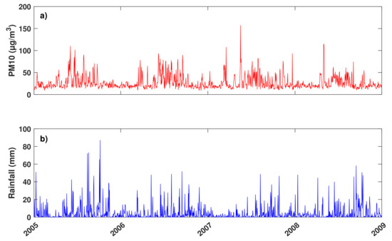
Figure 1.
Examples of synchronous time series between (a) daily average concentrations and (b) the daily sum of rainfall between 2005 and 2009.
2.2. Coherence Function
In order to analyze a potential interaction between two random processes, the second-order statistic is frequently performed [45]. Here, the coherence function is applied for estimating the correlations in the field of frequency between two processes and . The coherence function is computed as follows [46,47]:
where is the Fourier co-spectrum while and are respectively the Fourier spectra of and time series. According to sign, x and y may be uncorrelated (), perfectly correlated () or negatively correlated () [47].
2.3. Causality Framework
2.3.1. Convergent Cross Mapping
To investigate the causality in complex environments, the convergent cross mapping (CCM) method was introduced by Sugihara et al. [35]. This approach is based on the state space reconstruction (SSR) technique which is an advanced nonparametric technique [48]. To detect the interactions between nonlinear time series, the SSR technique became an efficient framework after the introduction of the embedding theory by Takens [49]. Hence, based on the simplex projection proposed by Sugihara and May [50], the CCM was developed and applied for nonlinear dynamic systems to study the relationship between two variables by using time-delayed embedding to reconstruct two shadow manifolds of X and Y [48].
Considering two time series X and Y of length L, which are presented as follows [48]:
By forming the lagged coordinate vectors of X and Y, the shadow attractor manifold and can be reconstructed by the following [48]:
where to , E is the embedding dimension, which represents the size of the time window, and the time lag is positive. There are E-dimensional points between the first lagged coordinate and the last, i.e., . From the results of Sugihara and May [50], the smallest bounding simplex is formed from the closest neighbors, so that the simplex can contain E-dimensional points. Therefore, an essential numerical limit on the potential embedding dimension E is needed. For n observations, the analysis requires observations to characterize the historical dynamics and at least one observation to quantify the estimated values, hence [51].
From the cross mapping, a library with L points from may be employed to supply estimates of L points for the original time series Y. Then, the ability of the L cross-mapped estimates from X to describe the L true value from Y can be quantified by the Pearson correlation coefficient which is defined as follows:
represents the predictive skills, i.e., the strength of influences from one variable to another variable, and ranges from 0 to 1. Hence, if Y has a causal impact on X, then will converge to , and should converge to . In theory, the CCM correlation should increase to L until infinity but in reality, the forecast skill of the cross-map estimates from X to Y can only reach a plateau [48].
2.3.2. Information Transfer
Another way to detect causality in stochastic dynamical systems is the information transfer method proposed by San Liang [52]. According to San Liang [53], for a two-dimensional system as follows:
represents the white noises, and are functions of X and t. Liang and Kleeman demonstrated that the rate of information flowing from to is the following according to Shannon entropy [53]:
where represents the marginal density of while is the mathematical expectation (units). Equation (6) naturally incorporates the rigorous principle of causality. Thereafter, this was improved by San Liang [36] with a concise formula. Thus, for two time series and , the estimate of the maximum likelihood of the information flow rate from to is expressed as follows [36]:
with the sample covariance between and , the covariance between and , and the difference approximation of using the Euler forward scheme with [36]. is in nats per unit time (e.g., nats per day) with “nat” for natural unit of information. When , does not cause ; if not, it is causal. If means that functions to make more uncertain, while indicates that tends to stabilize [36]. A recent study has shown that , arbitrarily termed Liang’s causality, is a good way to estimate the sign of the information flow [54].
To better quantify the strength of the causality between two variables, a new approach to normalize the information flow formula proposed by San Liang [36] is introduced by Bai et al. [37]:
where is the mathematical expectation, the marginal density of and [52]. According to Bai et al. [37], the stochastic effects is equal to:
, arbitrarily termed Bai’s causality, quantifies the importance of the information flow from to in comparison to other stochastic processes [37]. Contrary to , will always be positive due the absolute value applied during the normalization. For more details on information transfer theory and normalization computations, refer to San Liang [36,55] and Bai et al. [37].
3. Results and Discussion
3.1. Coherence Function Analysis
To assess an eventual relationship between and data in a dynamic way, the coherence function is firstly used. Figure 2 shows the coherence function for a frequency range Hz.
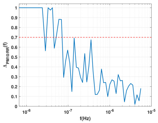
Figure 2.
The coherence function in semilogx plot of synchronous measurements between and over 11 years. The red horizontal dashed line indicates the significant correlation threshold ( 0.70) [47].
Overall, one can notice there is a correlation between and in the frequency domain. However, this correlation decreases as the frequency increases. Many peaks exceed the significant correlation threshold ( 0.70) introduced by Calif and Schmitt [47] at Hz corresponding to months (2.2 years). At Hz corresponding to months, is between 50% and 70%. goes below 40% at Hz corresponding to days. These results show that for small time-scales, the interactions between and seem weak.
The coherence function analysis is an efficient method to highlight the dynamic correlation between and . Nevertheless, as correlation does not imply causality but causation implies correlation, this method may not be suitable to exhibit causality [52]. In the correlation analysis, it lacks the needed asymmetry or directedness between dynamic events [37] and the mirage correlation might not be detected [56]. Consequently, other approaches which aim to detect the causal relationship between concentrations and values will be used.
3.2. Causality Analysis
3.2.1. Overall Analysis
In order to detect the causal nexus between concentrations and values, the CCM and the information transfer methods are performed. To apply the CCM frame, one must first estimate the optimal embedding dimension (E) and the time lag (). As E depends on many factors, i.e., system complexity, time series length L and noise [57], it is therefore crucial to compute it in the most rigorous way. This is the reason why the algorithm proposed by Wallot and Mønster [58] is used. This latter is based on the average mutual information and the false nearest neighbors to determine respectively and E values. For illustration purposes, Figure 3 shows the results achieved for data.
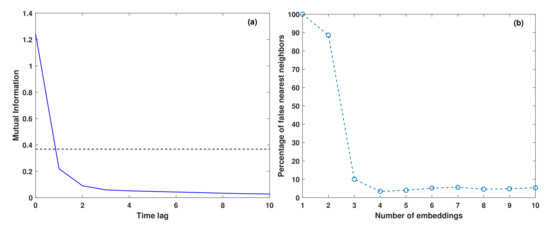
Figure 3.
Plots of (a) average mutual information and (b) false nearest neighbors for data. In (a) the black horizontal dashed line indicates the default threshold value.
In Figure 3a, one can notice that the average mutual information drops below the default threshold value at = 1 while in Figure 3b the percentage of false nearest neighbors remains almost constant from E = 3. The same pattern was observed for data. Thus, = 1 and E = 3 were retained to compute the CCM. As regards the information transfer frame, this approach is a data-driven procedure. Figure 4 and Figure 5 illustrate the causality computation between and respectively with CCM and information transfer methods. One can notice that Figure 4 exhibits an unidirectional causality ( to ), while Figure 5 highlights a bidirectional causality ( to and to ).
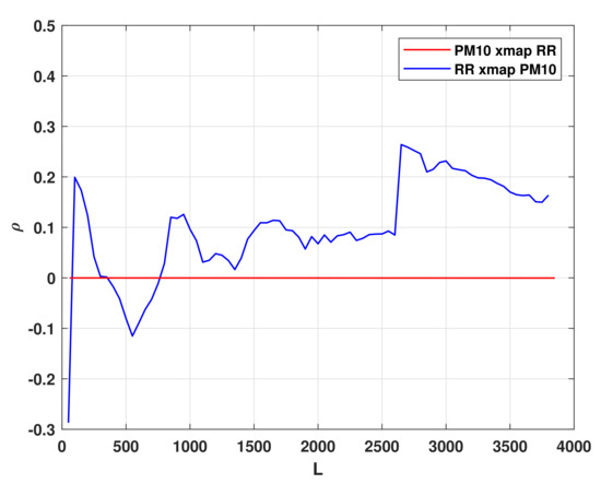
Figure 4.
Cross map between between and over 11 years.
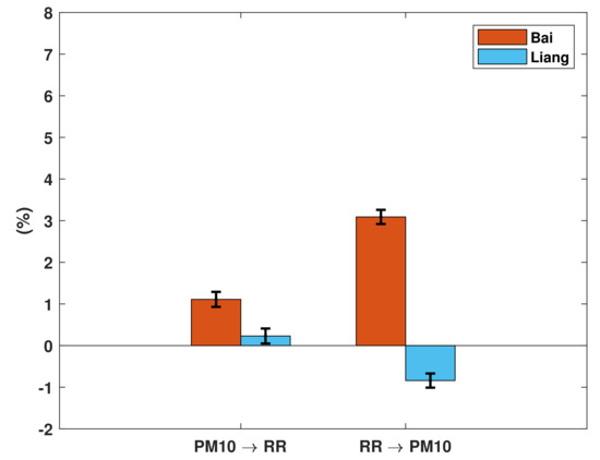
Figure 5.
Relative information flow from to and to over 11 years using Bai (, in orange) and Liang (, in blue) methods. The standard error (95% significance level) is represented by the whiskers.
For to , both Figures show the impact of the wet scavenging process [44]. In view of the studied data, it is difficult to define which scavenging process prevails between rainout or washout [59,60]. Everything will depend on location in the atmosphere. Indeed, the level of aerosols in and under the clouds during a rainy event determines whether the two phenomena occur simultaneously or not [61]. Contrary to the CCM, the information transfer shows simultaneously the strength () and the sign of the causality (). indicates that values tend to stabilize concentrations. This is in agreement with the literature because during and after a rainy episode, the levels will decrease in the atmosphere making their concentrations more homogeneous [62]. A recent study by Plocoste and Calif [54] between the and the atmospheric temperature (T) found that = 24.0% for the same period. This value is 8 times higher than the 3.0% obtained for . Thus, T values have more influence on concentrations than values. Such a difference may be due to the fact that wet deposition can only remove 30% of aerosols from the troposphere [63,64], while dry deposition can remove up to 70% [65]. In addition, during a rainy event, not all precipitation reaches the ground, as a certain fraction of the raindrops evaporate before reaching it.
As regards to , Figure 5 shows that also has an influence on behavior. Contrary to , which means that concentrations make values more uncertain. This may be due to nature which has several origins, i.e., mineral dust, marine aerosols or anthropogenic activity [7]. The impact of on T seems greater than the one of on as = 13.8% [54] and = 1.1%. Several studies have shown that concentrations induce a greenhouse effect which increases T values [54,66,67,68]. Conversely, ACIs are more complex mechanisms that involve several steps [8,9]. This may justify the weak information transfer from to . The author assumes that this weak exchange coupled with the fact that it is necessary to determine several parameters to compute the CCM can explain the non-detection of this interaction by this approach (see Figure 4). Given the drawbacks of the CCM method, only the information transfer frame would be carried out for the remainder of the study.
3.2.2. Seasonal Analysis
In the literature, many studies have demonstrated the impact of aerosol properties on ACIs [7,8,69,70]. In the Caribbean area, African dust seasonality has a significant impact on concentrations and air quality [19,28,71]. The low dust season is from October to April, while the high dust season is from May to September [12,19,27,72,73]. The Caribbean also experiences a rainfall cycle [74,75]. Classically, the dry season occurs from January to March, while the wet season takes place from July to November [40]. A recent study by Plocoste et al. [44] showed that the dry season can be extended from December to June. To discuss the causal results between the African dust seasonality and the rainy seasonality, the descriptive statistics for and time series are presented in Table 1.

Table 1.
The arithmetic mean (), standard deviation () and Kurtosis (K) of and over 11 years, for low (October to April) and high (May to September) dust seasons, for dry (December to June) and wet (July to November) seasons, and for high dust dry (May to June) and high dust wet (July to September) seasons. N is the sample size.
As benchmarks, and data over 11 years are also computed. In statistical analysis, the mean, the standard deviation and the kurtosis are parameters which respectively highlight the trend, fluctuation and intermittency of the data. The more intermittent the time series, the higher their kurtosis (K) [76]. The results of Table 1 show that the seasonality is well marked with average values 1.5 and 1.7 times higher respectively for the high dust season and the wet season.
Figure 6a,b shows the results achieved according to African dust seasonality. In Figure 6a,b, one can notice that and are almost the same for both seasons. During the low dust season, aerosol is mainly composed of sea spray [70] and anthropogenic pollution [77] as dust storms are weak [15]. This is the reason why in Table 1 < . During high dust season, mineral dust coming from the dust belt in Africa is persistently added to this set of aerosols [78]. Despite this addition, influence on seems to remain the same during high dust season. One can observe that the whiskers are wider for the high season. This can be attributed to the inter-annual variability of African dust storms [79]. At first glance, it seems that there is no difference in impact on between low and high dust seasons.
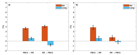
Figure 6.
Relative information flow from to and to using Bai (, in orange) and Liang (, in blue) methods for (a) low (October to April) and (b) high (May to September) dust seasons over 11 years. The standard error (95% significance level) is represented by the whiskers.
Regarding to (Figure 6a,b), the behavior is different as and are 4 times higher in the low season. During the high season, average is higher (see Table 1) but the wet scavenging process efficiency seems less significant. Two complementary approaches can explain the difference between both seasons. At the synoptic scale, mineral dusts are known to reduce precipitation once they are far away from their emissions sources [7,79,80,81]. From May to September, i.e., the high dust season, the large quantities of mineral dust from Africa both act on cloud microphysics and also reduce the convection process which enables their formation due to the extinction of solar radiation [7,8,80]. During this period, which coincides with the hurricane season [82,83], the rainfall will be mainly of synoptic origin as the African easterly waves always precede and follow a dusty event [84,85]. Furthermore, during the low season there are October and November, which are among the top five rainy months during the study period. October is even the rainiest month with a total of 2303 mm over 11 years [54]. All of these can explain the fact that the wet scavenging process is more significant in the low season than in the high one.
Figure 7a,b illustrates the results achieved according to the rainy seasonality. / and / are 5 times higher respectively in Figure 7a,b. Although June is known to be the dustiest month [78,86], the dry season is dominated by the low dust season as < and > (see Table 1). Thus, it is rather the marine aerosols which are predominant at this period. The rainfall is mainly of convective nature from December to June, i.e., mesoscale and local scale origin, allowing a longer residence time of in the atmosphere due to strong intermittency ( < in Table 1). Thus, and show the impact of aerosol properties on behavior between both seasons. As expected, the wet scavenging process, i.e., and , is more significant for the wet season due to higher and more persistent rainfall (see Table 1). On the other hand, influence on (/) is the lowest during that period. The more it rains, the greater the transfer of aerosols from the atmosphere to the ground. As a result, there will be less available to impact because their residence time in the atmosphere will be less. Furthermore, the strong atmospheric mixing generated by hurricane activity can also increase dispersion. It is important to underline that the whiskers are wider during the wet season. As this period mainly coincides with the high dust season and the hurricane activity, the author assumes that the inter-annual variability of African dust outbreaks coupled with dispersion can explain this behavior. For the wet scavenging process (), this phenomenon can be explained by the great variability of rainfall events in intensity and duration.
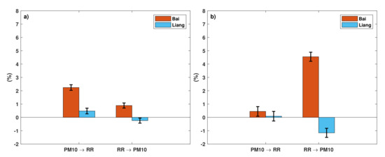
Figure 7.
Relative information flow from to and to using Bai (, in orange) and Liang (, in blue) methods for (a) dry (December to June) and (b) wet (July to November) seasons over 11 years. The standard error (95% significance level) is represented by the whiskers.
Based on the results obtained for African dust seasonality and rains seasonality, the high dust season is divided into two parts, i.e., the high dust dry (May to June) and high dust wet (July to September) seasons, in order to better assess the impact of concentrations on values. Figure 8a,b shows that influence on () is 3.5 times more significant during the high dust dry season, while the wet scavenging process () is slightly more important during the high dust wet season.
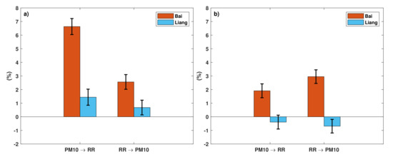
Figure 8.
Relative information flow from to and to using Bai (, in orange) and Liang (, in blue) methods for (a) high dust dry (May to June) and (b) high dust wet (July to September) seasons over 11 years. The standard error (95% significance level) is represented by the whiskers.
In Figure 8a,b, one can notice that the () make () more fluctuating in the high dust dry season (), while they homogenize them during the high dust wet season ( ). The author assumes that the residence time of in the atmosphere coupled with intermittency may explain this behavior. Indeed, Table 1 shows that and statistical parameters values between both periods are of the same order of magnitude, except for , which is 6 times higher during the high dust dry period. In Figure 8a, the impact of on is greater than in Figure 6b. Thus, these results show that during the same season, the impact of mineral dust on can evolve. In addition to their residence time in the atmosphere aforementioned, the chemical properties of mineral dust may also affect clouds characteristics. During the high dust season, dust storms can come from different parts of Africa [15]. Mineral dust chemical characteristics will strongly depend on the soils’ nature from which they originate [87,88,89]. A recent study showed that and broadly follow the same temporal pattern in the Caribbean area [78]. The highest values correspond to the highest values. Hence, dust outbreaks will bring of mineral origin. It is well known that is a better indicator of CCN activity than [90,91]. The CCN activity is determined by the aerosol number concentrations, which determine the cloud drop number concentrations. There is a good correlation between and CCN when all particles are small (near 0.1 m), but once some of them are large (>1 m) this correlation breaks. This is due to the fact that the mass of 1000 0.1 m particles equals the mass of one 1 m particle. As the high dust dry season corresponds to the highest concentrations (see Table 1), will also be significantly present. Even if the available data are not conducive to investigate this phenomenon, the author assumes that CCN activity could be more important during this period due to the strong presence of related to African dust.
4. Conclusions
The aim of this study was to assess the interactions between and rainfall () using ground-based measurements. To carry out this analysis, concentrations and values from Guadeloupe archipelago were used. Our results highlighted the feedback between and data. In other words, influence ( to ), while induce the wet scavenging process ( to ). We found that rainfall seasonality has a huge impact on wet scavenging process. During the wet season, this phenomenon is 5 times more significant, making concentrations more homogeneous. African dust seasonality also acts on behavior. During the first part of the high dust season, influence on is 2.5 times higher than in the low dust season, making values more heterogeneous. The highest wet scavenging process and the greatest impact of on correspond to the maximum average of and respectively. According to the author, these results highlight two types of causality: a direct causality ( to ) and an indirect causality ( to ). Indeed, the intensity and duration of rainfall events will have a direct impact on concentrations. On the other hand, the seasonal variation of concentrations will be an indicator of the presence of other smaller mineral particles conducive to acting as CCN.
To conclude, the results of this study showed the natural balance that exists to harmonize the climate. Thus, the entropy framework is a robust approach to quantify the behavior of atmospheric processes using ground-based measurements. Nothing is done at random to maintain the earth’s balance. Indeed, if mineral dusts were predominant during the dry season, it would accentuate the drought, while if the marine aerosols were predominant during the wet season, it would accentuate the rainfall, which would lead to more landslides due to soil saturation with water. In future research, we will examine the impact of climate change on CCN activity using number concentration.
Funding
The present study has no external funding.
Institutional Review Board Statement
Not applicable.
Informed Consent Statement
Not applicable.
Data Availability Statement
The data presented are available on request from the corresponding author. The data are not publicly available due to privacy or ethical reasons.
Acknowledgments
The author would like to thank the Guadeloupe air quality network (Gwad’Air) and the French Met Office (Météo France Guadeloupe) for providing air quality and meteorological data.
Conflicts of Interest
The author declares no conflict of interest.
References
- Kaufman, Y.J.; Tanré, D.; Boucher, O. A satellite view of aerosols in the climate system. Nature 2002, 419, 215–223. [Google Scholar] [CrossRef] [PubMed]
- Koch, D.; Menon, S.; Del Genio, A.; Ruedy, R.; Alienov, I.; Schmidt, G.A. Distinguishing aerosol impacts on climate over the past century. J. Clim. 2009, 22, 2659–2677. [Google Scholar] [CrossRef]
- Rosenfeld, D.; Sherwood, S.; Wood, R.; Donner, L. Climate effects of aerosol-cloud interactions. Science 2014, 343, 379–380. [Google Scholar] [CrossRef] [PubMed]
- Dickerson, R.; Kondragunta, S.; Stenchikov, G.; Civerolo, K.; Doddridge, B.; Holben, B. The impact of aerosols on solar ultraviolet radiation and photochemical smog. Science 1997, 278, 827–830. [Google Scholar] [CrossRef] [PubMed]
- Moosmüller, H.; Chakrabarty, R.; Arnott, W. Aerosol light absorption and its measurement: A review. J. Quant. Spectrosc. Radiat. Transf. 2009, 110, 844–878. [Google Scholar] [CrossRef]
- Albrecht, B.A. Aerosols, cloud microphysics, and fractional cloudiness. Science 1989, 245, 1227–1230. [Google Scholar] [CrossRef] [PubMed]
- Andreae, M.; Rosenfeld, D. Aerosol–cloud–precipitation interactions. Part 1. The nature and sources of cloud-active aerosols. Earth-Sci. Rev. 2008, 89, 13–41. [Google Scholar] [CrossRef]
- Fan, J.; Wang, Y.; Rosenfeld, D.; Liu, X. Review of aerosol–cloud interactions: Mechanisms, significance, and challenges. J. Atmos. Sci. 2016, 73, 4221–4252. [Google Scholar] [CrossRef]
- Li, Z.; Lau, W.M.; Ramanathan, V.; Wu, G.; Ding, Y.; Manoj, M.; Liu, J.; Qian, Y.; Li, J.; Zhou, T.; et al. Aerosol and monsoon climate interactions over Asia. Rev. Geophys. 2016, 54, 866–929. [Google Scholar] [CrossRef]
- Twomey, S. The influence of pollution on the shortwave albedo of clouds. J. Atmos. Sci. 1977, 34, 1149–1152. [Google Scholar] [CrossRef]
- Rosenfeld, D. TRMM observed first direct evidence of smoke from forest fires inhibiting rainfall. Geophys. Res. Lett. 1999, 26, 3105–3108. [Google Scholar] [CrossRef]
- Prospero, J.M.; Collard, F.X.; Molinié, J.; Jeannot, A. Characterizing the annual cycle of African dust transport to the Caribbean Basin and South America and its impact on the environment and air quality. Glob. Biogeochem. Cycles 2014, 28, 757–773. [Google Scholar] [CrossRef]
- Clergue, C.; Dellinger, M.; Buss, H.; Gaillardet, J.; Benedetti, M.; Dessert, C. Influence of atmospheric deposits and secondary minerals on Li isotopes budget in a highly weathered catchment, Guadeloupe (Lesser Antilles). Chem. Geol. 2015, 414, 28–41. [Google Scholar] [CrossRef]
- Rastelli, E.; Corinaldesi, C.; Dell’Anno, A.; Martire, M.L.; Greco, S.; Facchini, M.C.; Rinaldi, M.; O’Dowd, C.; Ceburnis, D.; Danovaro, R. Transfer of labile organic matter and microbes from the ocean surface to the marine aerosol: An experimental approach. Sci. Rep. 2017, 7, 11475. [Google Scholar] [CrossRef]
- Euphrasie-Clotilde, L.; Plocoste, T.; Feuillard, T.; Velasco-Merino, C.; Mateos, D.; Toledano, C.; Brute, F.N.; Bassette, C.; Gobinddass, M. Assessment of a new detection threshold for PM10 concentrations linked to African dust events in the Caribbean Basin. Atmos. Environ. 2020, 224, 117354. [Google Scholar] [CrossRef]
- Artíñano, B.; Salvador, P.; Alonso, D.G.; Querol, X.; Alastuey, A. Anthropogenic and natural influence on the PM10 and PM2.5 aerosol in Madrid (Spain). Analysis of high concentration episodes. Environ. Pollut. 2003, 125, 453–465. [Google Scholar] [CrossRef]
- Lewis, E.R.; Schwartz, S.E. Sea Salt Aerosol Production: Mechanisms, Methods, Measurements, and Models—A Critical Review; American Geophysical Union: Washington, DC, USA, 2004; Volume 152. [Google Scholar]
- Schulz, M.; de Leeuw, G.; Balkanski, Y. Sea-salt aerosol source functions and emissions. In Emissions of Atmospheric Trace Compounds; Springer: Berlin/Heidelberg, Germany, 2004; pp. 333–359. [Google Scholar]
- Prospero, J.M.; Delany, A.C.; Delany, A.C.; Carlson, T.N. The Discovery of African Dust Transport to the Western Hemisphere and the Saharan Air Layer: A History. Bull. Am. Meteorol. Soc. 2021, 102, E1239–E1260. [Google Scholar] [CrossRef]
- Prospero, J.M.; Carlson, T.N. Vertical and areal distribution of Saharan dust over the western equatorial North Atlantic Ocean. J. Geophys. Res. 1972, 77, 5255–5265. [Google Scholar] [CrossRef]
- Tsamalis, C.; Chédin, A.; Pelon, J.; Capelle, V. The seasonal vertical distribution of the Saharan Air Layer and its modulation by the wind. Atmos. Chem. Phys. 2013, 13, 11235–11257. [Google Scholar] [CrossRef]
- Petit, R.; Legrand, M.; Jankowiak, I.; Molinié, J.; Asselin de Beauville, C.; Marion, G.; Mansot, J. Transport of Saharan dust over the Caribbean Islands: Study of an event. J. Geophys. Res. Atmos. 2005, 110, D18S09. [Google Scholar] [CrossRef]
- Jury, M.R.; Jiménez, A.T.N. Tropical Atlantic dust and the zonal circulation. Theor. Appl. Climatol. 2021, 143, 901–913. [Google Scholar] [CrossRef]
- Schepanski, K. Transport of mineral dust and its impact on climate. Geosciences 2018, 8, 151. [Google Scholar] [CrossRef]
- Does, M.V.D.; Korte, L.F.; Munday, C.I.; Brummer, G.J.A.; Stuut, J.B.W. Particle size traces modern Saharan dust transport and deposition across the equatorial North Atlantic. Atmos. Chem. Phys. 2016, 16, 13697–13710. [Google Scholar] [CrossRef]
- Mahowald, N.; Albani, S.; Kok, J.F.; Engelstaeder, S.; Scanza, R.; Ward, D.S.; Flanner, M.G. The size distribution of desert dust aerosols and its impact on the Earth system. Aeolian Res. 2014, 15, 53–71. [Google Scholar] [CrossRef]
- Velasco-Merino, C.; Mateos, D.; Toledano, C.; Prospero, J.M.; Molinie, J.; Euphrasie-Clotilde, L.; González, R.; Cachorro, V.E.; Calle, A.; Frutos, A.M.d. Impact of long-range transport over the Atlantic Ocean on Saharan dust optical and microphysical properties based on AERONET data. Atmos. Chem. Phys. 2018, 18, 9411–9424. [Google Scholar] [CrossRef]
- Plocoste, T.; Calif, R.; Jacoby-Koaly, S. Temporal multiscaling characteristics of particulate matter PM10 and ground-level ozone O3 concentrations in Caribbean region. Atmos. Environ. 2017, 169, 22–35. [Google Scholar] [CrossRef]
- Cujia, A.; Agudelo-Castañeda, D.; Pacheco-Bustos, C.; Teixeira, E.C. Forecast of PM10 time-series data: A study case in Caribbean cities. Atmos. Pollut. Res. 2019, 10, 2053–2062. [Google Scholar] [CrossRef]
- Mauger, G.S.; Norris, J.R. Meteorological bias in satellite estimates of aerosol-cloud relationships. Geophys. Res. Lett. 2007, 34, 16. [Google Scholar] [CrossRef]
- Myhre, G.; Stordal, F.; Johnsrud, M.; Kaufman, Y.; Rosenfeld, D.; Storelvmo, T.; Kristjansson, J.E.; Berntsen, T.K.; Myhre, A.; Isaksen, I.S. Aerosol-cloud interaction inferred from MODIS satellite data and global aerosol models. Atmos. Chem. Phys. 2007, 7, 3081–3101. [Google Scholar] [CrossRef]
- Costantino, L.; Bréon, F.M. Analysis of aerosol-cloud interaction from multi-sensor satellite observations. Geophys. Res. Lett. 2010, 37, 11. [Google Scholar] [CrossRef]
- Seinfeld, J.H.; Bretherton, C.; Carslaw, K.S.; Coe, H.; DeMott, P.J.; Dunlea, E.J.; Feingold, G.; Ghan, S.; Guenther, A.B.; Kahn, R.; et al. Improving our fundamental understanding of the role of aerosol- cloud interactions in the climate system. Proc. Natl. Acad. Sci. USA 2016, 113, 5781–5790. [Google Scholar] [CrossRef]
- Wehbe, Y.; Tessendorf, S.A.; Weeks, C.; Bruintjes, R.; Xue, L.; Rasmussen, R.; Lawson, P.; Woods, S.; Temimi, M. Analysis of aerosol–cloud interactions and their implications for precipitation formation using aircraft observations over the United Arab Emirates. Atmos. Chem. Phys. 2021, 21, 12543–12560. [Google Scholar] [CrossRef]
- Sugihara, G.; May, R.; Ye, H.; Hsieh, C.h.; Deyle, E.; Fogarty, M.; Munch, S. Detecting causality in complex ecosystems. Science 2012, 338, 496–500. [Google Scholar] [CrossRef]
- San Liang, X. Unraveling the cause-effect relation between time series. Phys. Rev. E 2014, 90, 052150. [Google Scholar] [CrossRef]
- Bai, C.; Zhang, R.; Bao, S.; San Liang, X.; Guo, W. Forecasting the tropical cyclone genesis over the Northwest Pacific through identifying the causal factors in cyclone–climate interactions. J. Atmos. Ocean. Technol. 2018, 35, 247–259. [Google Scholar] [CrossRef]
- Peel, M.C.; Finlayson, B.L.; McMahon, T.A. Updated world map of the Köppen-Geiger climate classification. Hydrol. Earth Syst. Sci. 2007, 11, 1633–1644. [Google Scholar] [CrossRef]
- Plocoste, T.; Calif, R.; Jacoby-Koaly, S. Multi-scale time dependent correlation between synchronous measurements of ground-level ozone and meteorological parameters in the Caribbean Basin. Atmos. Environ. 2019, 211, 234–246. [Google Scholar] [CrossRef]
- Bertin, A.; Frangi, J. Contribution to the study of the wind and solar radiation over Guadeloupe. Energy Convers. Manag. 2013, 75, 593–602. [Google Scholar] [CrossRef]
- Plocoste, T.; Pavón-Domínguez, P. Multifractal detrended cross-correlation analysis of wind speed and solar radiation. Chaos Interdiscip. J. Nonlinear Sci. 2020, 30, 113109. [Google Scholar] [CrossRef]
- Winstanley, D. Rainfall patterns and general atmospheric circulation. Nature 1973, 245, 190–194. [Google Scholar] [CrossRef]
- Johnson, R.H.; Ciesielski, P.E. Rainfall and radiative heating rates from TOGA COARE atmospheric budgets. J. Atmos. Sci. 2000, 57, 1497–1514. [Google Scholar] [CrossRef]
- Plocoste, T.; Carmona-Cabezas, R.; Gutiérrez de Ravé, E.; Jimnez-Hornero, F.J. Wet scavenging process of particulate matter (PM10): A multivariate complex network approach. Atmos. Pollut. Res. 2021, 12, 101095. [Google Scholar] [CrossRef]
- Burton, T.; Jenkins, N.; Sharpe, D.; Bossanyi, E. Wind Energy Handbook; John Wiley & Sons: Hoboken, NJ, USA, 2011. [Google Scholar]
- Papoulis, A.; Pillai, S.U. Probability, Random Variables, and Stochastic Processes; Tata McGraw-Hill Education: New York, NY, USA, 2002. [Google Scholar]
- Calif, R.; Schmitt, F.G. Multiscaling and joint multiscaling description of the atmospheric wind speed and the aggregate power output from a wind farm. Nonlinear Process. Geophys. 2014, 21, 379–392. [Google Scholar] [CrossRef]
- Liu, H.; Lei, M.; Zhang, N.; Du, G. The causal nexus between energy consumption, carbon emissions and economic growth: New evidence from China, India and G7 countries using convergent cross mapping. PLoS ONE 2019, 14, e0217319. [Google Scholar] [CrossRef] [PubMed]
- Takens, F. Detecting strange attractors in turbulence. In Dynamical Systems and Turbulence, Warwick 1980; Springer: Berlin/Heidelberg, Germany, 1981; pp. 366–381. [Google Scholar]
- Sugihara, G.; May, R.M. Nonlinear forecasting as a way of distinguishing chaos from measurement error in time series. Nature 1990, 344, 734–741. [Google Scholar] [CrossRef] [PubMed]
- Clark, A.T.; Ye, H.; Isbell, F.; Deyle, E.R.; Cowles, J.; Tilman, G.D.; Sugihara, G. Spatial convergent cross mapping to detect causal relationships from short time series. Ecology 2015, 96, 1174–1181. [Google Scholar] [CrossRef] [PubMed]
- San Liang, X. Information flow within stochastic dynamical systems. Phys. Rev. E 2008, 78, 031113. [Google Scholar] [CrossRef] [PubMed]
- San Liang, X. The Liang-Kleeman information flow: Theory and applications. Entropy 2013, 15, 327–360. [Google Scholar] [CrossRef]
- Plocoste, T.; Calif, R. Is there a causal relationship between Particulate Matter (PM10) and air Temperature data? An analysis based on the Liang–Kleeman information transfer theory. Atmos. Pollut. Res. 2021, 12, 101177. [Google Scholar] [CrossRef]
- San Liang, X. Normalizing the causality between time series. Phys. Rev. E 2015, 92, 022126. [Google Scholar] [CrossRef]
- Chen, Z.; Xu, B.; Cai, J.; Gao, B. Understanding temporal patterns and characteristics of air quality in Beijing: A local and regional perspective. Atmos. Environ. 2016, 127, 303–315. [Google Scholar] [CrossRef]
- Ye, H.; Deyle, E.R.; Gilarranz, L.J.; Sugihara, G. Distinguishing time-delayed causal interactions using convergent cross mapping. Sci. Rep. 2015, 5, 14750. [Google Scholar] [CrossRef]
- Wallot, S.; Mønster, D. Calculation of Average Mutual Information (AMI) and False-Nearest Neighbors (FNN) for the estimation of embedding parameters of multidimensional time series in Matlab. Front. Psychol. 2018, 9, 1679. [Google Scholar] [CrossRef]
- Pillai, P.S.; Babu, S.S.; Moorthy, K.K. A study of PM, PM10 and PM2.5 concentration at a tropical coastal station. Atmos. Res. 2002, 61, 149–167. [Google Scholar] [CrossRef]
- Bayraktar, H.; Turalioğlu, F.S.; Tuncel, G. Average mass concentrations of TSP, PM10 and PM2.5 in Erzurum urban atmosphere, Turkey. Stoch. Environ. Res. Risk Assess. 2010, 24, 57–65. [Google Scholar] [CrossRef]
- Sonwani, S.; Kulshrestha, U.C. PM10 carbonaceous aerosols and their real-time wet scavenging during monsoon and non-monsoon seasons at Delhi, India. J. Atmos. Chem. 2019, 76, 171–200. [Google Scholar] [CrossRef]
- Tiwari, S.; Chate, D.; Pragya, P.; Ali, K.; Bisht, D.S. Variations in mass of the PM10, PM2.5 and PM 1 during the monsoon and the winter at New Delhi. Aerosol Air Qual. Res. 2012, 12, 20–29. [Google Scholar]
- Murakami, M.; Kimura, T.; Magono, C.; Kikuchi, K. Observations of precipitation scavenging for water-soluble particles. J. Meteorol. Soc. Jpn. Ser. II 1983, 61, 346–358. [Google Scholar] [CrossRef][Green Version]
- Schumann, T. Large discrepancies between theoretical and field-determined scavenging coefficients. J. Aerosol Sci. 1989, 20, 1159–1162. [Google Scholar] [CrossRef]
- McClintock, M.; McDowell, W.; González, G.; Schulz, M.; Pett-Ridge, J. African dust deposition in Puerto Rico: Analysis of a 20-year rainfall chemistry record and comparison with models. Atmos. Environ. 2019, 216, 116907. [Google Scholar] [CrossRef]
- Plocoste, T.; Calif, R.; Euphrasie-Clotilde, L.; Brute, F.N. Investigation of local correlations between particulate matter (PM10) and air temperature in the Caribbean basin using Ensemble Empirical Mode Decomposition. Atmos. Pollut. Res. 2020, 11, 1692–1704. [Google Scholar] [CrossRef]
- Plocoste, T.; Pavón-Domínguez, P. Temporal scaling study of particulate matter (PM10) and solar radiation influences on air temperature in the Caribbean basin using a 3D joint multifractal analysis. Atmos. Environ. 2020, 222, 117115. [Google Scholar] [CrossRef]
- Plocoste, T. Multiscale analysis of the dynamic relationship between particulate matter (PM10) and meteorological parameters using CEEMDAN: A focus on “Godzilla” African dust event. Atmos. Pollut. Res. 2022, 13, 101252. [Google Scholar] [CrossRef]
- Sherwood, S.C. Aerosols and ice particle size in tropical cumulonimbus. J. Clim. 2002, 15, 1051–1063. [Google Scholar] [CrossRef]
- Kristensen, T.B.; Müller, T.; Kandler, K.; Benker, N.; Hartmann, M.; Prospero, J.M.; Wiedensohler, A.; Stratmann, F. Properties of cloud condensation nuclei (CCN) in the trade wind marine boundary layer of the western North Atlantic. Atmos. Chem. Phys. 2016, 16, 2675–2688. [Google Scholar] [CrossRef]
- Plocoste, T.; Calif, R. Spectral Observations of PM10 Fluctuations in the Hilbert Space. In Functional Calculus; IntechOpen: London, UK, 2019; pp. 1–13. [Google Scholar]
- Plocoste, T.; Calif, R.; Euphrasie-Clotilde, L.; Brute, F.N. The statistical behavior of PM10 events over guadeloupean archipelago: Stationarity, modelling and extreme events. Atmos. Res. 2020, 241, 104956. [Google Scholar] [CrossRef]
- Plocoste, T.; Carmona-Cabezas, R.; Jiménez-Hornero, F.J.; Gutiérrez de Ravé, E.; Calif, R. Multifractal characterisation of particulate matter (PM10) time series in the Caribbean basin using visibility graphs. Atmos. Pollut. Res. 2021, 12, 100–110. [Google Scholar] [CrossRef]
- Martinez, C.; Goddard, L.; Kushnir, Y.; Ting, M. Seasonal climatology and dynamical mechanisms of rainfall in the Caribbean. Clim. Dyn. 2019, 53, 825–846. [Google Scholar] [CrossRef]
- Martinez, C.; Kushnir, Y.; Goddard, L.; Ting, M. Interannual variability of the early and late-rainy seasons in the Caribbean. Clim. Dyn. 2020, 55, 1563–1583. [Google Scholar] [CrossRef]
- Windsor, H.; Toumi, R. Scaling and persistence of UK pollution. Atmos. Environ. 2001, 35, 4545–4556. [Google Scholar] [CrossRef]
- Plocoste, T.; Dorville, J.F.; Monjoly, S.; Jacoby-Koaly, S.; André, M. Assessment of Nitrogen Oxides and Ground-Level Ozone behavior in a dense air quality station network: Case study in the Lesser Antilles Arc. J. Air Waste Manag. Assoc. 2018, 68, 1278–1300. [Google Scholar] [CrossRef]
- Euphrasie-Clotilde, L.; Plocoste, T.; Brute, F.N. Particle Size Analysis of African Dust Haze over the Last 20 Years: A Focus on the Extreme Event of June 2020. Atmosphere 2021, 12, 502. [Google Scholar] [CrossRef]
- Gavrouzou, M.; Hatzianastassiou, N.; Gkikas, A.; Korras-Carraca, M.B.; Mihalopoulos, N. A global climatology of dust aerosols based on satellite data: Spatial, seasonal and inter-annual patterns over the period 2005–2019. Remote. Sens. 2021, 13, 359. [Google Scholar] [CrossRef]
- Rosenfeld, D. Smoke and desert dust stifle rainfall, contribute to drought and desertification. Arid. News Lett. 2001, 49, 265. [Google Scholar]
- Rosenfeld, D.; Rudich, Y.; Lahav, R. Desert dust suppressing precipitation: A possible desertification feedback loop. Proc. Natl. Acad. Sci. USA 2001, 98, 5975–5980. [Google Scholar] [CrossRef]
- Tartaglione, C.A.; Smith, S.R.; O’Brien, J.J. ENSO impact on hurricane landfall probabilities for the Caribbean. J. Clim. 2003, 16, 2925–2931. [Google Scholar] [CrossRef]
- Dunion, J.P. Rewriting the climatology of the tropical North Atlantic and Caribbean Sea atmosphere. J. Clim. 2011, 24, 893–908. [Google Scholar] [CrossRef]
- Karyampudi, V.M.; Palm, S.P.; Reagen, J.A.; Fang, H.; Grant, W.B.; Hoff, R.M.; Moulin, C.; Pierce, H.F.; Torres, O.; Browell, E.V.; et al. Validation of the Saharan dust plume conceptual model using lidar, Meteosat, and ECMWF data. Bull. Am. Meteorol. Soc. 1999, 80, 1045–1076. [Google Scholar] [CrossRef]
- Plocoste, T.; Carmona-Cabezas, R.; Jiménez-Hornero, F.J.; Gutiérrez de Ravé, E. Background PM10 atmosphere: In the seek of a multifractal characterization using complex networks. J. Aerosol Sci. 2021, 155, 105777. [Google Scholar] [CrossRef]
- Zuidema, P.; Alvarez, C.; Kramer, S.J.; Custals, L.; Izaguirre, M.; Sealy, P.; Prospero, J.M.; Blades, E. Is summer African dust arriving earlier to Barbados? The updated long-term in situ dust mass concentration time series from Ragged Point, Barbados, and Miami, Florida. Bull. Am. Meteorol. Soc. 2019, 100, 1981–1986. [Google Scholar] [CrossRef]
- Negral, L.; Moreno-Grau, S.; Moreno, J.; Querol, X.; Viana, M.; Alastuey, A. Natural and anthropogenic contributions to PM10 and PM2.5 in an urban area in the western Mediterranean coast. Water Air Soil Pollut. 2008, 192, 227–238. [Google Scholar] [CrossRef]
- Perez, L.; Tobias, A.; Querol, X.; Künzli, N.; Pey, J.; Alastuey, A.; Viana, M.; Valero, N.; González-Cabré, M.; Sunyer, J. Coarse particles from Saharan dust and daily mortality. Epidemiology 2008, 19, 800–807. [Google Scholar] [CrossRef] [PubMed]
- Vanderstraeten, P.; Lénelle, Y.; Meurrens, A.; Carati, D.; Brenig, L.; Delcloo, A.; Offer, Z.Y.; Zaady, E. Dust storm originate from Sahara covering Western Europe: A case study. Atmos. Environ. 2008, 42, 5489–5493. [Google Scholar] [CrossRef]
- Yao, X.; Fang, M.; Chan, C.K.; Ho, K.; Lee, S. Characterization of dicarboxylic acids in PM2.5 in Hong Kong. Atmos. Environ. 2004, 38, 963–970. [Google Scholar] [CrossRef]
- Huang, G.; Cheng, T.; Zhang, R.; Tao, J.; Leng, C.; Zhang, Y.; Zha, S.; Zhang, D.; Li, X.; Xu, C. Optical properties and chemical composition of PM2.5 in Shanghai in the spring of 2012. Particuology 2014, 13, 52–59. [Google Scholar] [CrossRef]


Publisher’s Note: MDPI stays neutral with regard to jurisdictional claims in published maps and institutional affiliations. |
© 2022 by the author. Licensee MDPI, Basel, Switzerland. This article is an open access article distributed under the terms and conditions of the Creative Commons Attribution (CC BY) license (https://creativecommons.org/licenses/by/4.0/).