Error Features in Predicting Typhoon Winds: A Case Study Comparing Simulated and Measured Data

Abstract

Simulating a typhoon’s wind field via mesoscale models is important in terms of providing not only the guidelines for urban planning and onshore/offshore constructions, but also the provision of insight into the dynamics and thermodynamics of tropical cyclone systems. Therefore, the errors that are contained in simulation results were investigated in the present study, in association with large-scale meteorological patterns and localized wind conditions in the typhoon boundary layer. In detail, the full-set three-dimensional simulations of three typhoon cases were carried out in order to provide the typhoon wind fields that were required to compare with the observations that were obtained through land weather stations and offshore buoys. Although the reliability of typhoon simulations has been thoroughly investigated, the previous works mostly concentrated on the configurations and dynamic core of the model. The present study reveals, however, the influences of the characteristics of the specific weather system on the simulation’s results, which provides the foundation for the proposition of empirical corrections to improve the mesoscale simulation results of typhoon wind fields without updating the model’s algorithm.

1. Introduction

Intensive tropical cyclones, which are also referred to as typhoons in the northwest Pacific, are generally associated with extreme winds, intense rainfalls and storm tides, which can cause severe damages to onshore and offshore structures. China is one of the countries that suffers from damages that are induced by typhoons. Particularly, landfalling typhoons pose major threats to the coastal buildings and offshore structures in typhoon-prone regions of China. In each year, around 7–9 typhoons [1] make landfall along the southeastern coast of China. Hence, it is of critical importance to reliably predict typhoon wind fields in order to provide guidelines, not only for urban planning [2] but also for the design of onshore and offshore structures [3,4]. In addition, the simulation of typhoon wind fields is useful in the investigation of the dynamics and thermodynamics of the tropical cyclone system [5,6].

Among the three-dimensional wind field simulation tools that are available in the fields of meteorology and wind engineering, the mesoscale numerical weather prediction (NWP) model is one of the most popular data sources for deriving the information from a tropical cyclone wind field. The weather research and forecast (WRF) model [7,8], as one mesoscale NWP tool, is widely used for the simulation of typhoon wind fields due to its advanced numerical configuration and trustworthy physical parameterization schemes [9]. Given its popularity [10], previous studies have been carried out in order to assess the errors in the WRF-simulated wind field. In fact, the influences of the microphysics scheme [11,12], planetary boundary layer scheme [13], surface layer parameterization [14,15] and cumulus parameterization [16] on the simulation of wind and precipitation fields [17] have been systematically investigated, based on the observations that have been obtained from the weather station network and remote sensing instruments, such as satellites and radars. In addition, the grid resolution [16] and the reanalysis data [18] that are used to generate the boundary and initial condition for a WRF simulation are also included in the investigations concerning the discrepancies between simulation results and observations. In the present simulation of typhoon wind fields, analyses of the simulation’s accuracy and reliability have been carried out in order to optimize the configuration of the WRF model to reproduce the track and intensity of typhoons that were extracted from the best-track database [19].

Considering the importance of the three-dimensional wind field to the tropical cyclone for academic investigations and practical applications in the assessment of the damages that are induced by typhoons, efforts have been made to enhance the reliability and accuracy of typhoon simulations [20]. Even though a series of studies [21,22] have revealed the influences of various factors of different weather systems on the WRF simulation, the main foci of previous studies have been placed on the configurations or the dynamic core algorithm of the model [21,22]. The influences of the characteristics of the weather system on the discrepancies between the simulated and observed tropical cyclone wind fields still demands further investigation, especially a quantitative study helping to assess the errors in the prediction where observations are not available. For one thing, the present study shows the features that a weather system should acquire in order for contemporary modelling techniques to successfully capture its general and detailed patterns. More importantly, analyses of the errors in the simulation’s results shed light onto empirical corrections that could be made to the simulation’s results. In order to improve the simulation’s reliability and accuracy, it is certain that the NWP model itself could be re-coded in order to utilize the most up-to-date understanding of the meteorology dynamic. However, a more practical way to produce reliable estimates based on the existing operational model is to empirically correct the simulation’s results based on simulated large-scale weather patterns and localized wind conditions. The present study may be inadequate to improve the core algorithm of the NWP model, but it provides a useful reference for the empirical corrections that may be made to the results of the existing model. In fact, the present study takes the typhoon as an exemplar weather system in order to discern the features of the WRF simulation’s errors and their relationship with the large-scale meteorological environment and localized wind conditions. It should be noted that the present study is only the first attempt of the authors to relate the discrepancies between the WRF-simulated and observed tropical cyclone wind fields with the known large-scale weather patterns and localized wind conditions. Furthermore, the findings are obtained from the WRF simulations of only three selected typhoon cases which occurred in the South China Sea. In addition, the present study employs a perfectly-structured Rankine vortex in order to initialize the development of the tropical cyclone, which could lead to discrepancies between the simulated and observed wind fields in the tropical cyclones’ boundary layers. It is therefore indeed a long-term, on-going endeavor of the authors to suggest more comprehensive empirical corrections based on more WRF simulations covering a wider range of weather systems.

Following this introduction, Section 2 describes the configurations that were used to run the simulations of three historical typhoons. Section 3 briefly summarizes the comparisons of the WRF simulation results, in terms of time and the series of wind speeds and directions, with the measurements that were taken from both land weather stations and offshore buoy measurements at sparse locations. Based on the error statistics report, the error features and their connections to the large-scale meteorological patterns and the localized wind conditions are discussed in Section 4. The concluding remarks are presented in Section 5.

2. Numerical Simulation

The WRF model is a third-generation non-hydrostatic mesoscale numerical weather prediction software package that was developed by the National Center for Atmospheric Research (NCAR), the National Centers for Environmental Prediction (NCEP) and other relevant research institutes [7,8]. In the present study, the model version 3.4 is utilized.

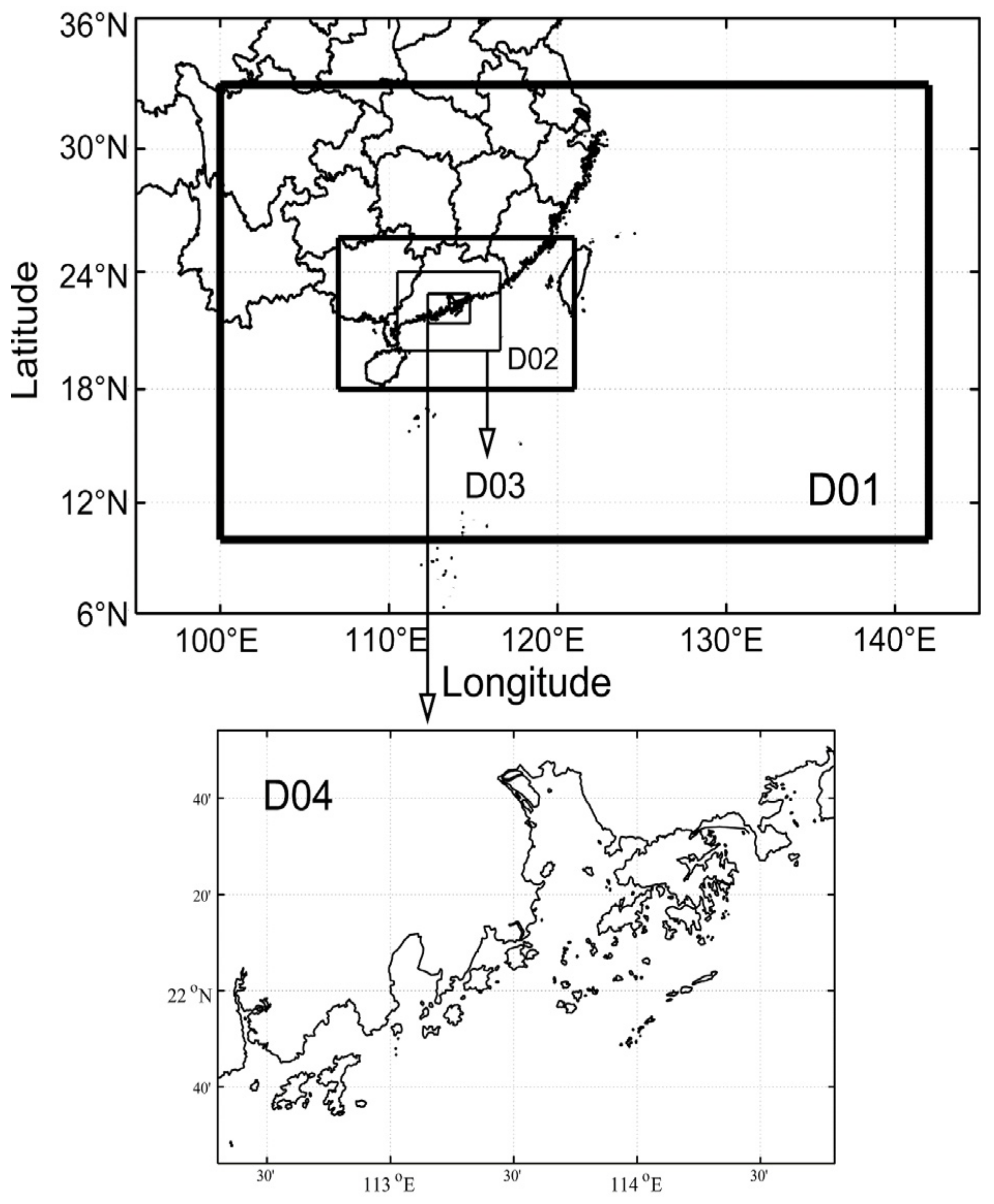
2.1. Simulation Domain

In the WRF simulation, a nested-domain configuration with four inter-chained domains was employed, as shown in Figure 1. In detail, the outermost domain, D01, covers most of the northwest Pacific (latitudes spanning from $10°\mathrm{N}$ to$33°\mathrm{N}$ and longitudes spanning from $100°\mathrm{E}$ to $142°\mathrm{E}$). The horizontal grid spacing and the number of grid points for D01 are 27 km and 149 × 89, respectively. The second domain, D02, covers the entire southeast of China (latitudes spanning from $18°\mathrm{N}$ to $25.7°\mathrm{N}$ and longitudes spanning from $107°\mathrm{E}$ to $121°\mathrm{E}$). The horizontal grid spacing and the number of grid points for D02 are 9 km and 150 × 90, respectively. The third domain, D03, covers the Guangdong Province (latitudes spanning from $20°\mathrm{N}$ to $24°\mathrm{N}$ and longitudes spanning from $110.5°\mathrm{E}$ to $116.6°\mathrm{E}$). The horizontal grid spacing and the number of grid points for D03 are 3 km and 198 × 141, respectively. The innermost domain, D04, focuses on the coasts of Shenzhen and Hong Kong (latitudes spanning from $21.4°\mathrm{N}$ to $22.9°\mathrm{N}$and longitudes spanning from$112.3°\mathrm{E}$to$114.8°\mathrm{E})$. The horizontal grid spacing and the number of grid points for D04 are 1 km and 240 × 159, respectively. In all domains, 44 layers were established in order to discretize the atmosphere spanning from 10 hPa to 1000 hPa in the vertical direction and the vertical spacing increased with the heights in order to make sure that the near-surface flow in the typhoon boundary layer was simulated with higher resolutions.

2.2. Boundary and Initial Condition

The historical reanalysis data that were used to initiate the WRF simulation are maintained by the European Centre for Medium-Range Weather Forecasts (ECMWF) and are available publicly on the Internet (European Centre for Medium-Range Weather Forecasts: http://apps.ecmwf.int/datasets/data/interim-full-daily/levtype=sfc/ accessed on 31 December 2020) [23]. The data is recorded four times (at 00, 06, 12 and 18 UTC) per day and includes all of the necessary meteorological variables that are required in order to initiate a WRF simulation. The horizontal resolution of the data is $0.75°\times 0.75°$. The details of the ECMWF data that were used in the present study are shown in

Table 1. Details of ECMWF historical reanalysis data.

Parameter	Content
3D variables	U and V components of wind, temperature, relative humidity and geopotential height.
Pressure levels (hPa)	10, 20, 30, 50, 70, 100, 150, 200, 250, 300, 350, 400, 450, 500, 550, 600, 650, 700, 750, 800, 850, 900, 925, 950, 975, 1000
2D variables (Surface level)	10-m U and V components of wind, surface pressure, mean sea level pressure, skin temperature, 2-m temperature, 2-m relative humidity.
Areas	$100°\mathrm{E}–145°\mathrm{E},5°\mathrm{N}–35°\mathrm{N}$
Horizontal Resolution	$0.75°\times 0.75°$
Temporal interval	6 h

.

Using these ECMWF data, three historical typhoon cases were simulated. In detail, the Typhoon Kai-tak, Usagi and Vicente, which occurred during the years of 2012 and 2013, were simulated. The start and end moments of each typhoon simulation case, listed in

Table 2. Start and end points of the time periods in three typhoon cases.

Date (UTC)		Location	Maximum Wind Speed (m/s)	Central Pressure (hPa)
Typhoon Kai-tak
Start	08, 12 August 2012	$131.80°\mathrm{E}$, $16.60°\mathrm{N}$	13	1004
End	00, 18 August 2012	$102.60°\mathrm{E}$, $23.10°\mathrm{N}$	10	1000
Typhoon Usagi
Start	18, 16 September 2013	$132.40°\mathrm{E}$, $17.50°\mathrm{N}$	13	1006
End	00, 23 September 2013	$107.80°\mathrm{E}$, $24.80°\mathrm{N}$	10	1002
Typhoon Vicente
Start	06, 20 July 2012	$128.50°\mathrm{E}$, $14.80°\mathrm{N}$	13	1006
End	00, 25 July 2012	$105.10°\mathrm{E}$, $22.20°\mathrm{N}$	8	996

, were determined according to the best track data that is maintained by the Hong Kong Observatory.

2.3. Model Configuration

The initial meteorological fields that were extracted from the ECMWF data were relatively coarse in terms of their horizontal resolutions, which could have been problematic as the small-scale perturbations necessary for the typhoon genesis were absent. Following the common practice in the simulation of historical typhoons [24], a bogus tropical cyclone with a perfect structure was inserted into the initial field in order to force the genesis of a typhoon. In detail, using the numerical tool that is embedded in WRF software package [25,26], a three-dimensional Rankine vortex with predefined key parameters was inserted. The inserted Rankin vortex was defined by the longitude and latitude of the vortex center, the radius to the maximum wind speed (RMW) and the maximum sustainable wind speed [27]. The latitudes and longitudes of the center location of the bogus tropical cyclone and the maximum sustainable wind speeds were determined according to the best track records of historical typhoons, maintained by the Hong Kong Observatory. The RMW, on the other hand, can be estimated based on central pressures or maximum wind speeds using a series of empirical models [28]. Among the empirical models, the model that is recommended by Chang et al. was employed [29] in the present study in order to estimate the RMW according to the central pressure ${\mathrm{P}}_{\mathrm{c}}$ as shown in Equation (1).

$${\mathrm{R}}_{\max }=0.4785·{\mathrm{P}}_{\mathrm{c}}-413$$

(1)

In Equation (1), ${\mathrm{R}}_{\max }$ is the RMW (in the unit of km), ${\mathrm{P}}_{\mathrm{c}}$ is the central pressure (in the unit of hPa). Regarding the other model configurations that were used to run the WRF simulation in the present study, the details of these are summarized in

Table 3. Detailed settings of the WRF model. MM5: mesoscale model 5; YSU: Yonsei University; WSM3: WRF single-moment 3-class; RRTM: rapid radiative transfer model.

Domain	D01	D02	D03	D04
Configuration	4 nested domains, Mercator projection
Grid points	$103\times 119$	$231\times 315$	$384\times 210$	$273\times 318$
Time step	Adaptive time step (Courant, Friedrichs, Lewy number $\le$1.6)
Physics	Surface layer: MM5 scheme [30]
	Boundary layer: YSU scheme [31]
	Land surface model: MM5 5-layer thermal diffusion [32]
	Cumulus parameterization: Kain–Fritsch scheme [33]
	Microphysics: WSM3 scheme [34]
	Radiation physics: RRTM scheme [35]
FDDA (Four- dimensional data assimilation)	Spectral nudging [36]
	Variable		Nudging coefficient (${\mathrm{s}}^{-1}$)
	Wind speed		$3\times {10}^{-4}$
	Temperature		$1\times {10}^{-4}$
	Geopotential height		$1\times {10}^{-4}$
	Wave number (x)		4
	Wave number (y)		2

.

2.4. Post-Processing

After the model was configured, three historical typhoon cases were simulated in order to yield the typhoon wind fields within the specific periods (shown in Table 2). Since the bogus tropical cyclone, with a perfect but unrealistic vortex structure, was inserted into the initial field, the simulation results within the first 12 h were considered unreliable and hence discarded. After the first 12 h, the simulated typhoon wind fields were continuously recorded at a 3-min interval. In the discussion of the WRF simulation of wind fields, the results extracted from the D04 domain were post-processed in order to yield the profiles of the hourly mean wind speeds and directions at the locations of the land weather station and the offshore buoys, from which the observations were obtained for comparisons.

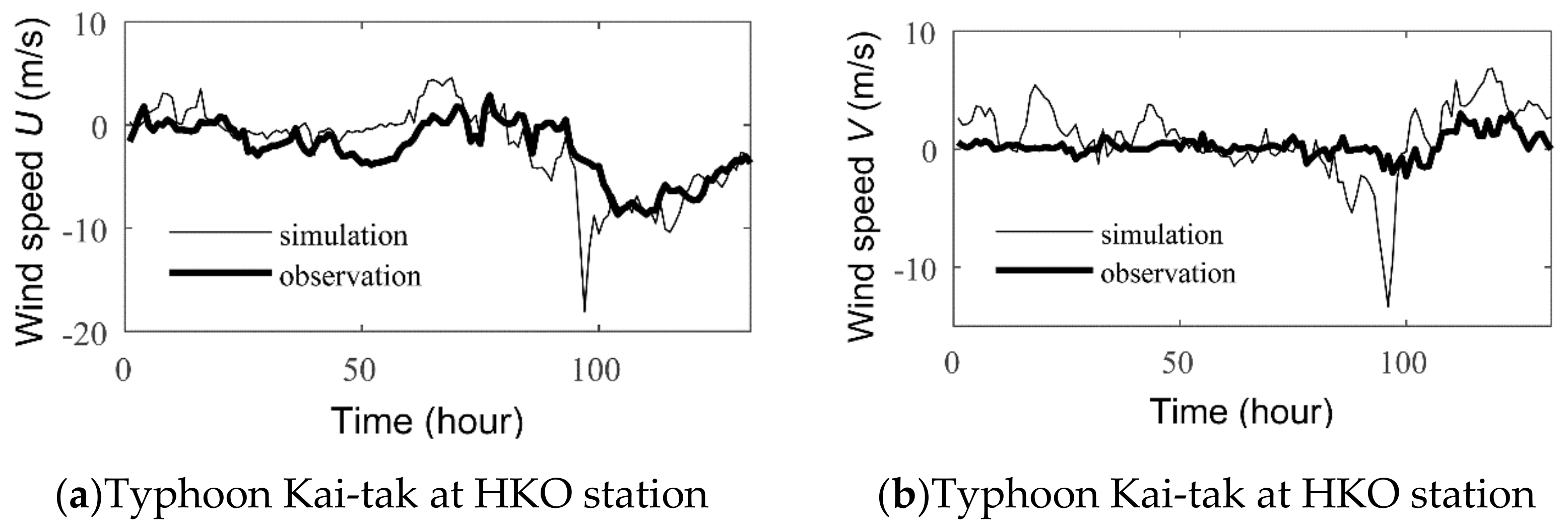
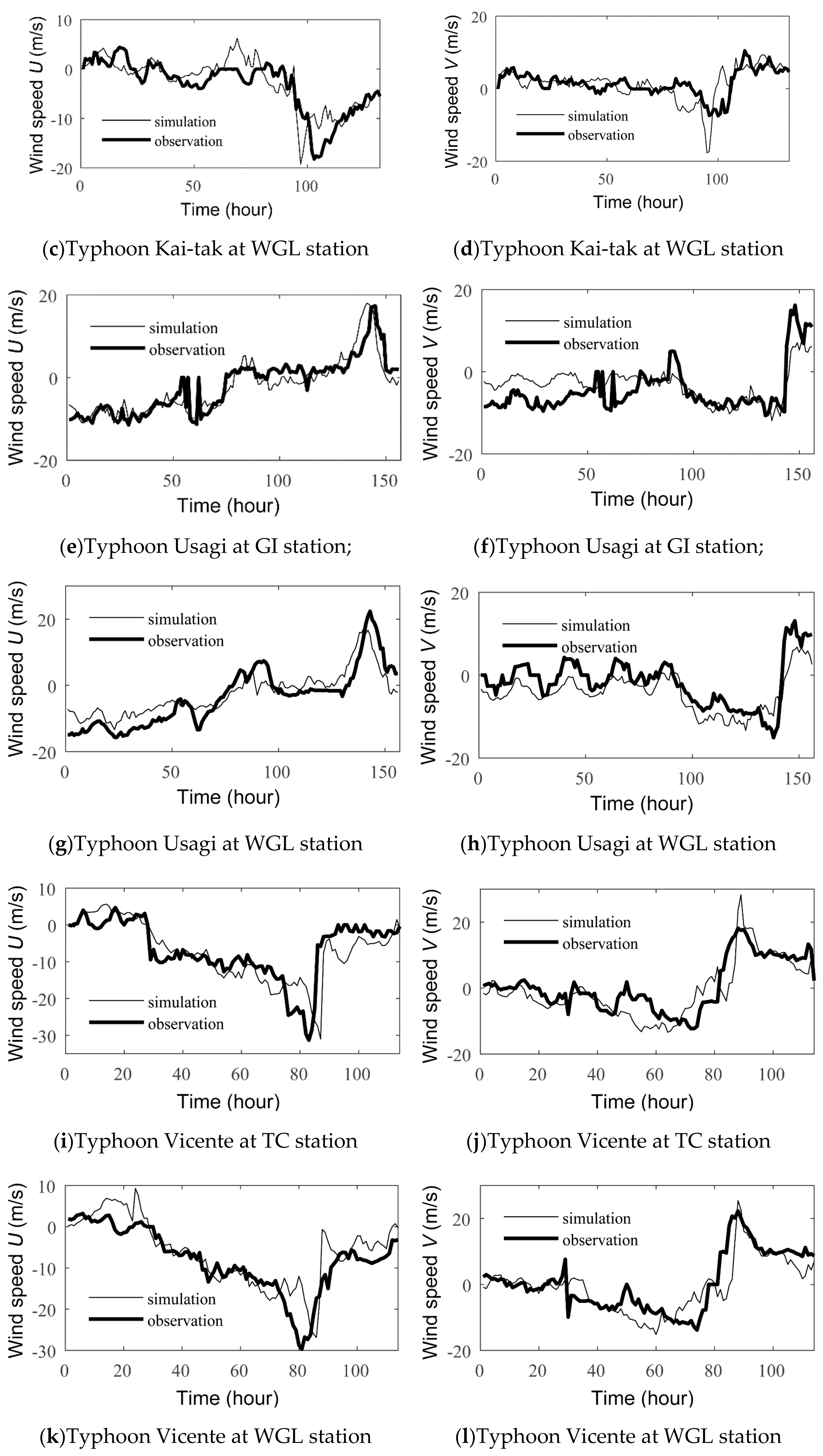
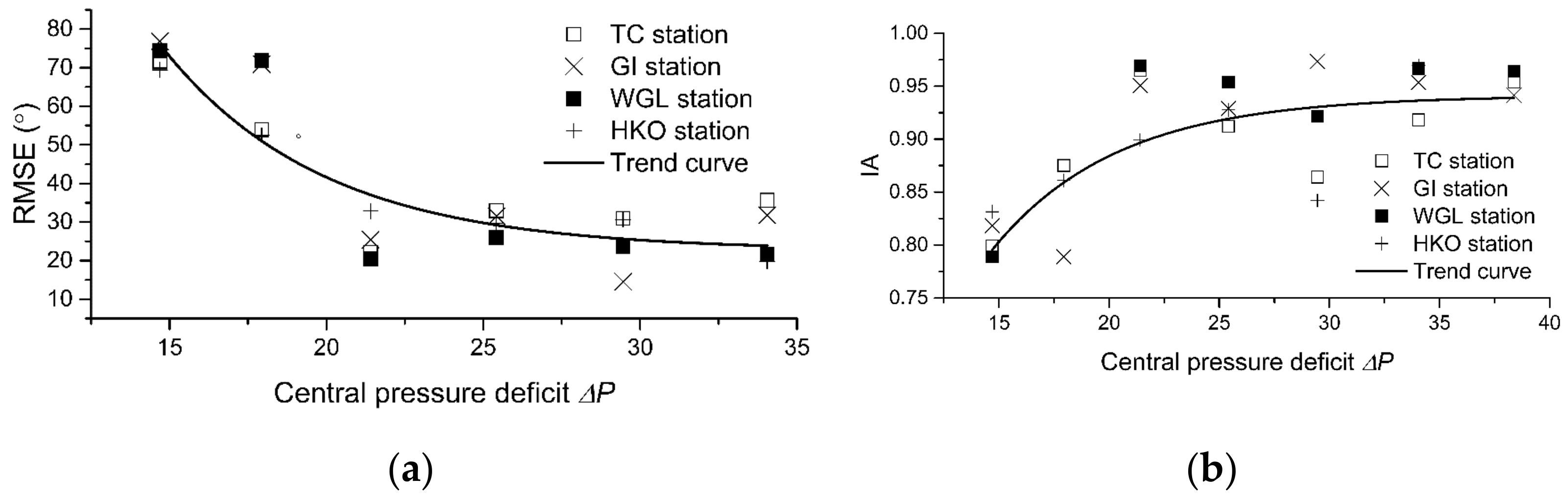
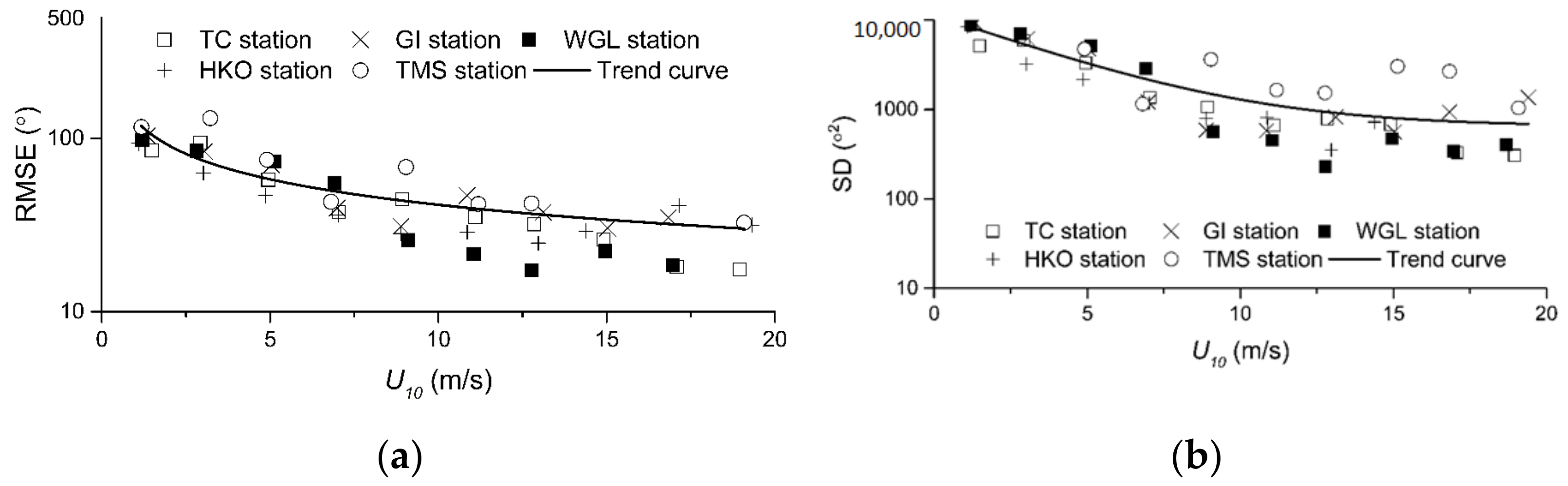
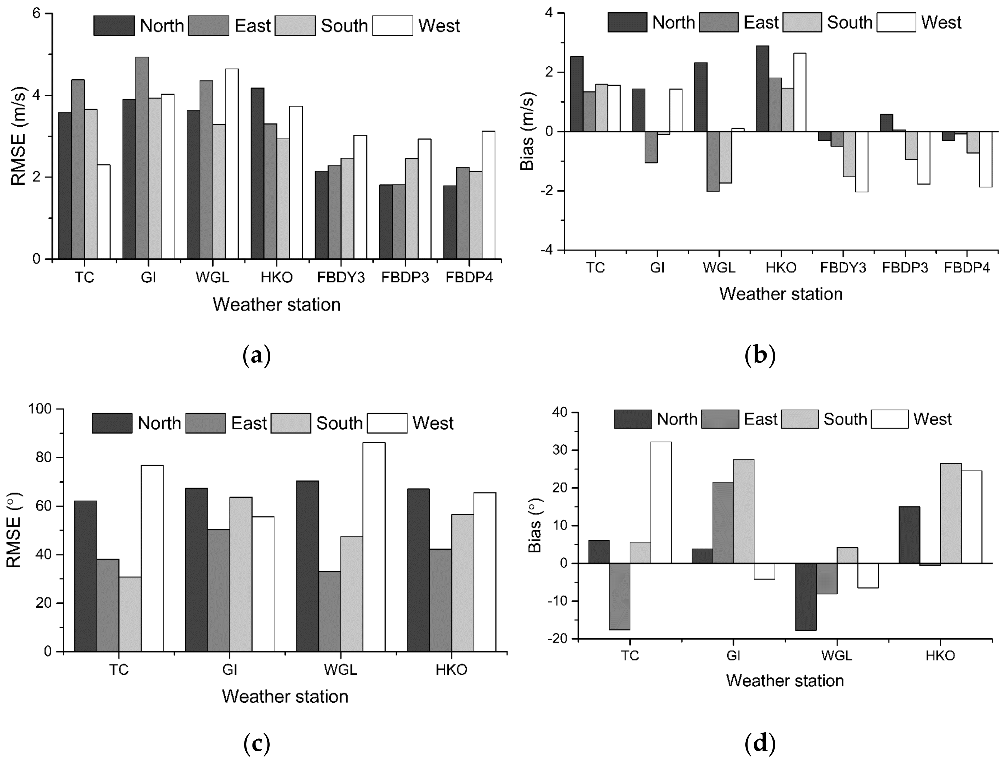
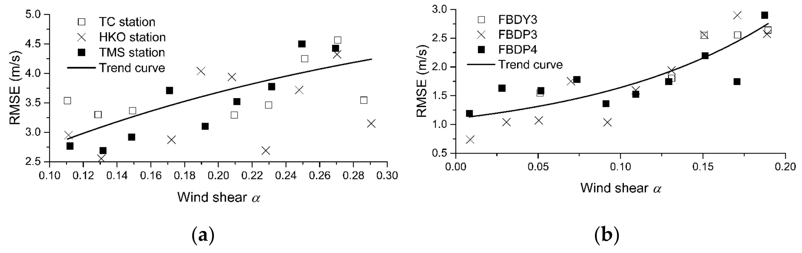
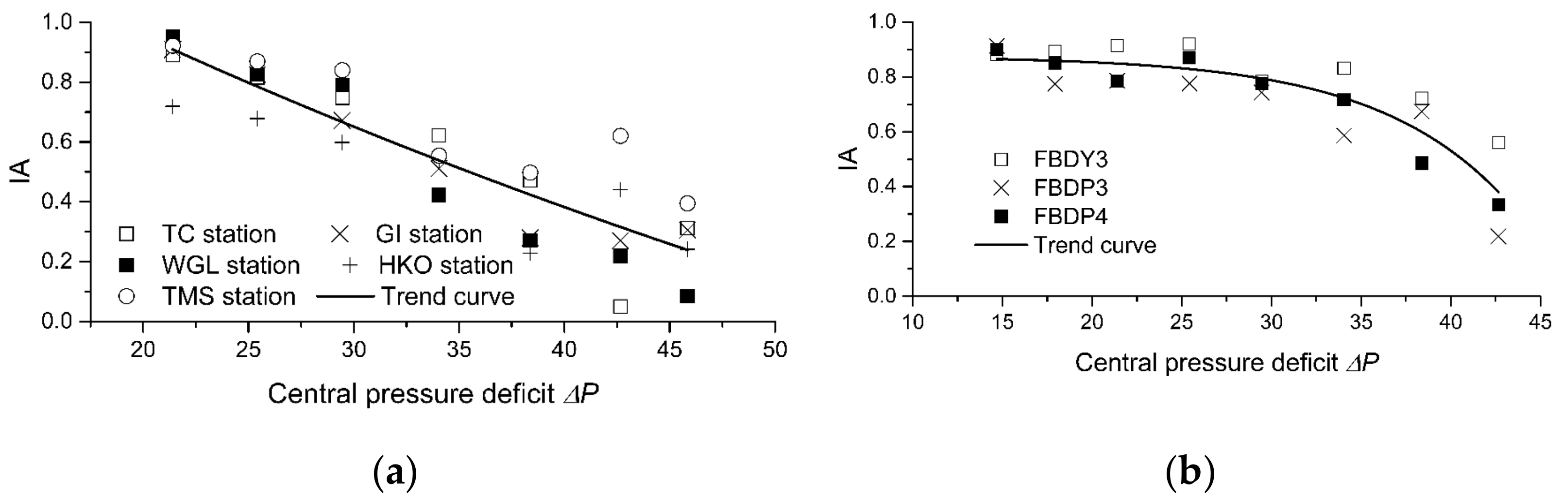
3. Error Statistics Report

Before further investigating the error features and their connections to large-scale meteorological patterns and localized wind conditions, the error statistics were reported through comparing the simulations to the observations. In detail, the hourly mean wind speeds and directions that were collected at five land weather stations, which are maintained by the Hong Kong Observatory, were employed. The hourly mean wind speeds at the sensor height (2 m) observed by the offshore buoys deployed by the Shenzhen Marine Observation and Prediction Center were also used. The relevant information regarding the weather station and offshore buoys is summarized in

Table 4. Details of the land weather station and offshore buoys.

Station Name	Position	Elevation above the Mean Sea Level (m)
Land weather station
Tate’s Cairn (TC)	$114.22°\mathrm{E}$$22.36°\mathrm{N}$	587
Green Island (GI)	$114.11°\mathrm{E}$$22.29°\mathrm{N}$	107
Waglan Island (WGL)	$114.30°\mathrm{E}$$22.18°\mathrm{N}$	83
Tai Mo Shan (TMS)	$114.12°\mathrm{E}$$22.41°\mathrm{N}$	966
Hong Kong Observatory (HKO)	$114.17°\mathrm{E}$$22.30°\mathrm{N}$	74
Offshore buoy
FBDY3	$114.52°\mathrm{E}$$22.57°\mathrm{N}$	2
FBDP3	$114.46°\mathrm{E}$$22.57°\mathrm{N}$	2
FBDP4	$114.49°\mathrm{E}$$22.53°\mathrm{N}$	2

and their geographic locations are shown in Figure 2.

It can be seen in Figure 2 that the TC and TMS stations, whose elevations above the mean sea level are 587 m and 966 m, respectively, are located in the mountainous region with complex land topographies. While the HKO station, FBDY3, FBDP3 and FBDP4 are near the shore. This shows the influence of land–sea transitions. The GI and WGL stations are sited on islands under the influence of offshore meteorological circulations. The enlarged surrounding environment for the HKO station and the WGL station are shown in Figure 3.

In order to make a direct comparison between the simulated and observed wind speeds and directions, the simulated typhoon wind fields that were extracted from the innermost domain (D04) were interpolated to the corresponding locations and heights using the cubic spline method [37]. Given that the wind field should vary smoothly in reality, the cubic spline interpolation produces an accurate and smooth estimate of both wind speeds and directions at the observation location. For the sake of brevity, only two comparisons, which were chosen randomly from all of the comparisons in each typhoon case, are illustrated in Figure 4 and Figure 5 in order to show the general accuracy of the simulation results.

In general, the comparisons that are shown in Figure 4 and Figure 5 reveal that the patterns, i.e., the occurrence location and magnitude of the peaks and valleys, are shared by both the simulated and observed wind velocities. Especially, the simulated wind velocities in the east–west and north–south directions, as demonstrated in Figure 4, and the magnitude of the simulated wind velocities, shown in Figure 5, are in a good agreement with the observations. Furthermore, the comparisons corresponding to the offshore buoys present better agreements than those corresponding to the land weather stations.

In order to quantify the discrepancies between the simulated and observed typhoon winds, five error indicators [3,38,39], namely the root mean square error ($\mathrm{RMSE}$), the $\mathrm{bias}$, the squared standard deviation ($\mathrm{SSD}$), the scatter index ($\mathrm{SI}$) and the index of agreement ($\mathrm{IA}$), were employed. The definitions of the five indicators are:

$$RMSE=\sqrt{{\displaystyle \sum }_{i=1}^n{\left(S_i-O_i\right)}^2/n}$$

(2)

$$Bias={\displaystyle \sum }_{i=1}^N\left(S_i-O_i\right)/n$$

(3)

$$SSD=RMS{E}^2-Bia{s}^2$$

(4)

$$SI=RMSE/\overline{O}$$

(5)

$$IA=1-\frac{n·RMS{E}^2}{{{\displaystyle \sum }}_{i=1}^n{\left(\left|S_i-\overline{O}\right|+\left|O_i-\overline{O}\right|\right)}^2}$$

(6)

In Equations (2)–(6), $\mathrm{n}$ represents the size of the sample dataset. ${\mathrm{S}}_{\mathrm{i}}$ and ${\mathrm{O}}_{\mathrm{i}}$ are the simulated and corresponding observed data. The overbar indicates the calculation of the mean. It should be noted that the simple arithmetic subtraction does not yield the difference between the simulated and observed wind directions. Following Carvalho et al. [40], the difference between the simulated and observed wind directions was calculated as,

$$S_i-O_i=\left({\theta }_s-{\theta }_o\right)\times \left[1-\frac{360}{\left|{\theta }_s-{\theta }_o\right|}\right], if \left|{\theta }_s-{\theta }_o\right|>180°$$

(7)

In Equation (7), ${\mathsf{\theta }}_{\mathrm{s}}$ is the simulated wind direction while ${\mathsf{\theta }}_{\mathrm{o}}$ is the observed wind direction. According to the definitions of the error indicators that are shown above, $\mathrm{RMSE}$ shows the deviation, in general, of the simulation results from the observed data. $\mathrm{Bias}$ was used in order to assess the trend of the deviation. $\mathrm{SSD}$ indicates the stability of the deviation and a lower $\mathrm{SSD}$ implies that the simulation captures the variations of the observed wind speed and direction and hence the physics were truthfully simulated. $\mathrm{SI}$, on the other hand, indicates the degree of dispersion. $\mathrm{IA}$ is a general index, varied from 0 to 1, which was used to indicate the degree of agreement between the simulated and observed data [41]. The five error indicators, calculated based on the simulation and observations corresponding to all three of the typhoon simulation cases, are summarized in

Table 5. Summary of the error indicators for the wind speed simulation.

Station	RMSE (m/s)	Bias (m/s)	SSD (${\mathbf{m}}^2/$${\mathbf{s}}^2$)	SI (m/s)	IA
TC	3.82	1.80	11.32	0.44	0.88
GI	4.26	−0.07	18.15	0.55	0.77
WGL	3.93	−0.67	15.01	0.44	0.87
HKO	3.43	2.05	7.53	0.93	0.72
TMS	4.30	0.64	18.12	0.42	0.88
FBDY3	2.30	−0.77	4.72	0.40	0.89
FBDP3	2.01	−0.17	4.00	0.46	0.84
FBDP4	2.16	−0.40	4.49	0.46	0.85

and

Table 6. Summary of the error indicators for the wind direction simulation.

Station	RMSE ($°$)	Bias ($°$)	SSD (${°}^2$)	SI ($°$)	IA
TC	51.35	−5.39	2607.90	0.37	0.92
GI	59.25	17.80	3193.30	0.41	0.92
WGL	55.78	−7.32	3057.60	0.43	0.91
HKO	55.72	8.68	3029.20	0.36	0.91

. The entire sample size that was used to calculate the error indicators for a single observation site was greater than 6300.

Table 5 and Table 6 quantitatively show how the simulated wind speeds and directions compare to the observations, in addition to Figure 4 and Figure 5. Consistent with the conclusion that was drawn from the comparisons that are shown in the figures, the error statistics report indicates that, in most case, the errors at the offshore buoys tended to be lower than those of the land weather stations. More specifically, the $\mathrm{RMSE}$, $\mathrm{bias}$ and $\mathrm{SSD}$ corresponding to the offshore buoys were lower than those corresponding to the land weather stations by ~45%, ~57% and ~69%, respectively. Such systematic differences may be connected to the difficulties in simulating the typhoon wind field over the complex land topography along the shore. The largest errors appeared at the TMS station showing the largest $\mathrm{RMSE}$ (4.30 m/s) and $\mathrm{SD}$ (18.12 ${\mathrm{m}}^2$/${\mathrm{s}}^2$) for wind speeds. Moreover, it was found that the $\mathrm{SI}$ corresponding to the wind speeds that were measured and simulated at the HKO station were larger than those of the other locations, showing a maximum value of 0.93 m/s, which could be attributed to the influence of the urban morphology surrounding the HKO station, as shown in Figure 3. In fact, the error variations that were exposed in the statistics report suggest that the reliability of the simulations of the wind speeds and directions is in connection to both the large-scale features of the typhoon systems and the localized wind conditions.

4. Discussion

Based on the error statistics that are reported in Section 3, the features of the errors in the simulated typhoon wind speeds and directions and their connections to both the large-scale meteorological pattern and localized wind conditions were investigated. Such an investigation builds the foundation for empirical corrections to be made to the WRF simulations of the tropical cyclone wind field, given the simulated general weather patterns and known localized wind conditions. In detail, the pressure deficit of a typhoon system and the distance from the observation location to the typhoon center were employed in order to show the influence of the large-scale meteorological pattern. The wind speeds and directions at 10 m height and the wind shear, on the other hand, were used as indicators in order to investigate the influence of the localized wind conditions.

4.1. Large-Scale Feature

In the present study, the pressure deficit and distance between the observation location and the typhoon’s center are discussed in connection with the error statistics that were calculated according to Equations (2)–(7). The central pressure deficit was calculated as,

$$\Delta P=P_b-P_c$$

(8)

In Equation (8), ${\mathrm{P}}_{\mathrm{c}}$ is the central pressure of a specific typhoon. ${\mathrm{P}}_{\mathrm{b}}$ shows the background sea-level pressure, equaling to 1013.25 hPa. The normalized distance is defined as,

$$r=\frac{R}{R_{max}}$$

(9)

In Equation (9), $\mathrm{R}$ represents the distance between the locations of the observations and the typhoon center, while ${\mathrm{R}}_{\max }$ is the RMW that is estimated based on the simulated central pressure of the typhoon according to Equation (1). In the calculation of the error indicators, the central pressure deficit is equally binned with a size varying from 3 hPa–5 hPa in order to ensure that the sample size for the calculation of the error indicator is meaningful and that the sample sizes for the calculation are all larger than 300. Similarly, the normalized distance was binned with a step varying from 2.5–3.5.

Using the indicators of $\Delta \mathrm{P}$ and $\mathrm{r}$, the error statistics of the simulated wind speeds and directions were plotted against $\Delta \mathrm{P}$ and $\mathrm{r}$, as shown in Figure 6, Figure 7, Figure 8 and Figure 9. The relationships between the error indicators and $\Delta \mathrm{P}$& $\mathrm{r}$ are revealed by the trend curves that have been fitted through the least square method [42].

According to Figure 6, it was found that the $\mathrm{IA}$ of the wind speeds over land and sea decreased with $\Delta \mathrm{P}$, which indicates that the degree of agreement between the simulated and observed data deteriorated with increasing typhoon intensity. The errors in the simulated wind directions, on the other hand, imply that the simulation of wind directions improved with increasing typhoon intensity, according to the decreasing $\mathrm{RMSE}$ and increasing $\mathrm{IA}$that are shown in Figure 7. One plausible explanation might be that the intensive typhoons are, in general, associated with more perfectly organized primary vortexes. In such cases, the variation in wind directions is relatively low and depends mainly on the large-scale meteorological pattern of the typhoon system. In other words, other small-scale factors influencing the wind directions are suppressed in an intensive typhoon, which makes the WRF simulation of wind directions more accurate.

As for the relationship between the error indicators and the normalized distance $\mathrm{r}$, it is evident from the data that are reported in Figure 8 and Figure 9 that the $\mathrm{RMSE}$ and $\mathrm{SD}$ of the wind speed simulations nonlinearly decreased with the increasing normalized distance. In other words, the error reduced when the typhoon was moving away from the observation site. In detail, the $\mathrm{RMSE}$ and $\mathrm{SD}$ in the bin of $25–30$ were less than, in general, those in the bin of $0–5$ by 57.99% and 83.85%, respectively. A striking feature is that the degree of agreement between the simulations and observations in terms of the wind directions over the land deteriorated with the increase in the $\mathrm{r}$ value. The $\mathrm{RMSE}$ of the wind direction, on the other hand, first increased when $\mathrm{r}$ varied in the range $0–20$, then decreased when $\mathrm{r}$ was in the range of $20–30$. More specifically, the largest $\mathrm{RMSE}$ appeared when the $\mathrm{r}$ value reached $15–18$, while the smallest $\mathrm{RMSE}$ occured in the bins of $0–5$ and $25–30$. It should be acknowledged that when the typhoon approaches the observation site, the air-land/sea momentum flux is influenced by the relative position of the observation site in a typhoon system [43]. The spatial variation in air-land/sea momentum fluxes is, however, simply parametrized according to the Monin–Obukhov similarity theory in a WRF simulation. Such parameterization is postulated to be inaccurate near the typhoon’s center. For example, Mohan et al. found that the external ocean mixing model, which provides additional adjustments to the surface heat/momentum fluxes parameterizations, enhanced the simulation of tropical cyclone intensities [44]. Compared to the error indicators of the wind speeds, the nonlinear variation in the errors of the wind directions indicates that the highest $\mathrm{RMSE}$ generally appears in the location with a distance of $15\mathrm{RMW}–20\mathrm{RMW}$ away from the typhoon’s center. In short, the variations of the error statistics that are revealed in Figure 8 and Figure 9 implies that the WRF simulations of the wind speeds over land and the sea are in better agreement with the observations when the typhoon’s center keeps a certain distance from the site.

In conclusion, the reliability of the WRF simulation’s results is under the influence of the large-scale meteorological pattern of a typhoon system. More specifically, the reliability of the simulated wind speeds decreases approaching the center of an intensive typhoon. The degree of agreement in the simulated and observed wind directions, however, presents a different trend. Moreover, the $\mathrm{RMSE}$ of the wind directions decreases with increased typhoon intensity and shows the highest value in a ring with a distance of $15\mathrm{RMW}–20\mathrm{RMW}$ away from the typhoon’s center.

4.2. Localized Wind Conditions

In addition to the large-scale meteorological pattern, the localized wind conditions, as indicated by the localized wind speeds and directions at 10 m and the shear in the wind profile, were included in our investigation. More specifically, the observed wind speeds (${\mathrm{U}}_{10}$) and directions (${\mathsf{\theta }}_{10}$) at 10 m at each observation site were employed in order to investigate the influence of the localized wind conditions. When determining the influence of ${\mathrm{U}}_{10}$, the observed ${\mathrm{U}}_{10}$ was binned with a step size of 2 m/s. In each bin, the error indicators were calculated in order to assess the model’s performance, as presented in Figure 10 and Figure 11.

According to the Figure 10 and Figure 11, it becomes clear that the simulation errors of the wind speeds increase with ${\mathrm{U}}_{10}$, whereas the errors in the simulated wind directions decrease exponentially with ${\mathrm{U}}_{10}$. Such difference is expected since, under the conditions of low wind speeds, the wind direction measurement and simulation are subjected to higher errors due to the fact that the weak winds are generally associated with unstable atmospheric regimes [14]. Given that the variation in the wind directions is higher in the convective boundary layer with unstable stratification, it is difficult for the model to reliably capture all of the variations in the wind directions. As for the errors in the simulation of the wind speeds, there seems to be, in Figure 10, a linear trend of the $\mathrm{bias}$ with the wind speeds; for the low wind speed bin ($<10\mathrm{m}/\mathrm{s}$), the $\mathrm{bias}$ tended to be negative and low; for the high wind speed bin ($\ge 10\mathrm{m}/\mathrm{s}$), it became positive and high. Therefore, it could be concluded that the WRF simulation, in most cases, tends to overestimate the wind strength in the typhoon’s boundary layer when ${\mathrm{U}}_{10}$ is above 10 m/s.

Figure 12 presents the wind speed and direction error variation with the observed wind directions at 10 m (${\mathsf{\theta }}_{10}$). The error statistics were binned into four sectors, according to ${\mathsf{\theta }}_{10}$, as: north (${\mathsf{\theta }}_{10}$ in the range between 315$°$ and 45$°$), east (${\mathsf{\theta }}_{10}$ in the range between 45$°$ and 135$°$), south (${\mathsf{\theta }}_{10}$ in the range between 135$°$ and 225$°$) and west (${\mathsf{\theta }}_{10}$ in the range between 225$°$ and 315$°$).

It can be found from the results that are reported in Figure 12 that the east sector shows the highest error for the simulated wind speeds at the TC and GI stations, while the west sector reveals the largest error in the wind speeds that were measured or simulated at the WGL station and at all three of the offshore buoys. Referring to Figure 2, it is suggested that the WRF model’s performance deteriorates when the wind flow is coming from the land–ocean interface, similar to the conclusions that have been found in the previous work [14]. As for the HKO station, the north sector is associated with highest errors in simulated wind speeds. Obviously, such errors could be attributed to the facts that the wind blowing from the north passes through complex urban morphology (the downtown area of Kowloon, Hong Kong) and that the WRF simulation of the urban canopy layer is always a challenge. Another interesting finding is that the simulations, on average, overestimated the wind speed over land and underestimated the wind speed over the sea. Previous studies [9,45] have explained that WRF presents a high wind speed bias over land, which is attributed to the exclusion of sub−grid orographic drag in the formulation of surface roughness lengths. Hence, such difference exposed in the Figure 12b may be explained by the drawback of the surface parameterizations, in which the topographic data underestimates the land−surface roughness while overestimates the sea−surface roughness. Comparing to the simulation of the wind speeds, the errors in the simulated wind directions show a different variation pattern. In detail, the north and west sectors show the highest errors over land, which are related to the weak northerly and westerly synoptic winds over the coast of China [46]. In addition, the $\mathrm{bias}$ of the wind direction is ranged from $~-20°$ to $~30°$ where the simulation results in the south sector always erroneously predicting the wind direction over land, according to Figure 12d.

In summary, Figure 12 implies a degradation of the WRF simulation results of wind speeds when the wind was coming from the land–ocean interface and from complex urban terrain. Moreover, it was found that the simulations, in most cases, overestimated the wind speed over land and underestimated the wind speed over the sea. The errors in the simulated wind directions, on the other hand, are related to the weak northerly and westerly synoptic winds over the coast of China, which are not properly simulated in the WRF model.

In addition to the wind speeds and directions, Wang and Jin found that wind shear might be a factor in influencing the performance of the WRF model [38]. Hence, the simulated and observed wind speeds and directions were binned according to wind shear ($\mathsf{\alpha }$) with a step size of 0.02. The wind shear was calculated as

$$\alpha =\frac{ln\left[U\left(z_2\right)/U\left(z_1\right)\right]}{ln\left(z_2/z_1\right)}$$

(10)

In Equation (6), $\mathrm{U}\left({\mathrm{z}}_2\right)$ and $\mathrm{U}\left({\mathrm{z}}_1\right)$ are the wind speeds at two different height levels (${\mathrm{z}}_2=120\mathrm{m},{\mathrm{z}}_1=6\mathrm{m})$, extracted from the simulated wind profile. In each bin, the error indicators corresponding to the wind speeds and directions were calculated and are shown in Figure 13 and Figure 14.

It was found from the data that are reported in Figure 13 and Figure 14 that the errors in the wind speed simulations increased while the errors in the simulated wind directions decreased with $\mathsf{\alpha }$. It should be noted that wind shear is mainly related to atmospheric stratification, the land/sea surface roughness and the magnitude of typhoon wind speeds [3]. Therefore, it is evident from the figures that it is still challenging for a mesoscale model to simulate wind velocities reliably when the magnitude of the wind velocity gradient is high. Such difficulties may be connected with the parameterizations of the land−surface process that are adopted in the WRF model. The $\mathrm{RMSE}$ and $\mathrm{bias}$ of the simulated wind directions, on the other hand, decreased with $\mathsf{\alpha }$, according to the data that are reported in Figure 14. It is speculated that the performance of the wind direction simulations, in essence, is related to the magnitude of the typhoon’s wind speed. Considering that $\mathsf{\alpha }$ increases with the wind speed under typhoon conditions, as concluded in previous studies [3], the magnitude of the typhoon wind speed, not the atmospheric stratification and the land or sea surface roughness, was found in the present study to directly influence the simulation of wind directions under typhoon conditions.

5. Conclusions

In the present study, the WRF simulations of three historical typhoon cases were conducted in order to provide typhoon wind fields for the discussion of the features of simulation errors. More specifically, the error statistics and their connections to the large-scale meteorological patterns and the localized wind conditions were investigated. Although a considerable number of previous studies have been carried out in order to assess and analyze the errors in the WRF simulation of typhoon wind fields, their main focuses were placed on the configuration of the model. In other words, the influences of the characteristics of a specific weather system, such as a typhoon, have not yet been a topic of systematical study. A quantitative investigation of the errors in the WRF simulation could be beneficial in (a) determining the reliability of WRF predictions under specific conditions and (b) developing an empirical correction of the WRF simulation of typhoon wind fields. It should be noted that it is the authors’ long-term and on-going aim to develop a comprehensive set of empirical corrections to be made to the WRF simulation results, in order to enhance the reliability and realism of the estimates of wind speeds and directions. The presently reported work is only a preliminary attempt, which will build the foundation for further endeavors, based on more WRF simulations covering a wider range of weather systems.

From the process of comparing simulations with observations that were obtained from inland weather stations and offshore buoys, it was found that the reliability of simulated wind speeds decreases approaching the center of an intensive typhoon. The degree of agreement in simulated and measured wind directions, however, presents a different trend. More specially, the $\mathrm{RMSE}$ of the wind direction error decreases with the typhoon’s intensity. In general, the influence of large-scale meteorological features on simulation errors, to a large extent, could be explained by the degree of organization in the typhoon’s main vortex and the spatial characteristics of the air–land–sea momentum flux.

In addition to the large-scale meteorological pattern, the localized wind conditions, as indicated by the wind speed and direction at 10 m and the wind shear were included in the investigation. In general, it was found that the errors in the simulated wind speeds exponentially increased with the magnitude of the wind speed at 10 m. The simulations, in most cases, overestimated the wind speed over land and underestimated the wind speed over the sea. The variations in the simulation’s errors for wind directions were found in association with weak northerly and westerly synoptic winds over the coast of China, which are not properly simulated by the WRF model. In addition to the localized wind speed and direction, the present study has quantitatively discerned, for the first time, that the simulation of wind speeds deviates from the observations with increasing wind shear. The simulation of wind directions, on the contrary, improves in the sheared wind flow.

It should be noted that the conclusions that were drawn from the present study are based on a few selected typhoon cases which occurred and were observed in the South China Sea and the findings are, therefore, primarily applicable for corrections that could be made to the mesoscale simulation of tropical cyclones, especially for the tropical cyclones that are observed in the South China Sea. Although the applicability of the present study is limited, it could shed light onto the corrections that may be made to the WRF forecasts of tropical cyclones.

References

1. China Meteorological Administration. The Tropical Cyclone Yearbook; China Meteorological Press: Beijing, China, 2014. [Google Scholar]
2. Liu, Y.; Chen, D.; Li, S.; Chan, P. Revised power-law model to estimate the vertical variations of extreme wind speeds in China coastal regions. J. Wind. Eng. Ind. Aerodyn. 2018, 173, 227–240. [Google Scholar] [CrossRef]
3. Liu, Y.; Chen, D.; Yi, Q.; Li, S. Wind Profiles and Wave Spectra for Potential Wind Farms in South China Sea. Part I: Wind Speed Profile Model. Energies 2017, 10, 125. [Google Scholar] [CrossRef] [Green Version]
4. Liu, Y.; Li, S.; Chan, P.W.; Chen, D. Empirical Correction Ratio and Scale Factor to Project the Extreme Wind Speed Profile for Offshore Wind Energy Exploitation. IEEE Trans. Sustain. Energy 2017, 9, 1030–1040. [Google Scholar] [CrossRef]
5. Sun, X.; Barros, A.P. High resolution simulation of tropical storm Ivan (2004) in the Southern Appalachians: Role of planetary boundary-layer schemes and cumulus parametrization. Q. J. R. Meteorol. Soc. 2014, 140, 1847–1865. [Google Scholar] [CrossRef]
6. Kim, D.; Jin, C.-S.; Ho, C.-H.; Kim, J.; Kim, J.-H. Climatological features of WRF-simulated tropical cyclones over the western North Pacific. Clim. Dyn. 2014, 44, 3223–3235. [Google Scholar] [CrossRef]
7. Grell, G.A.; Peckham, S.E.; Schmitz, R.; McKeen, S.A.; Frost, G.; Skamarock, W.C.; Eder, B. Fully coupled “online” chemistry within the WRF model. Atmos. Environ. 2005, 39, 6957–6975. [Google Scholar] [CrossRef]
8. Michalakes, J.; Dudhia, J.; Gill, D.; Klemp, J.; Skamarock, W. Design of a Next-Generation Regional Weather Research and Forecast Model; Towards Teracomputing 1998; World Scientific: River Edge, NJ, USA, 1998; pp. 117–124. [Google Scholar]
9. Jiménez, P.A.; Dudhia, J. Improving the representation of resolved and unresolved topographic effects on surface wind in the WRF model. J. Appl. Meteorol. Climatol. 2012, 51, 300–316. [Google Scholar] [CrossRef] [Green Version]
10. Papanastasiou, D.; Melas, D.; Lissaridis, I. Study of wind field under sea breeze conditions; an application of WRF model. Atmos. Res. 2010, 98, 102–117. [Google Scholar] [CrossRef]
11. Tao, W.-K.; Wu, D.; Lang, S.; Chern, J.-D.; Peters-Lidard, C.; Fridlind, A.; Matsui, T. High-resolution NU-WRF simulations of a deep convective-precipitation system during MC3E: Further improvements and comparisons between Goddard microphysics schemes and observations. J. Geophys. Res. Atmos. 2016, 121, 1278–1305. [Google Scholar] [CrossRef]
12. Sun, J.; He, H.; Hu, X.; Wang, D.; Gao, C.; Song, J. Numerical Simulations of Typhoon Hagupit (2008) Using WRF. Weather. Forecast. 2019, 34, 999–1015. [Google Scholar] [CrossRef]
13. Banks, R.F.; Tiana-Alsina, J.; Baldasano, J.M.; Rocadenbosch, F.; Papayannis, A.; Solomos, S.; Tzanis, C.G. Sensitivity of boundary-layer variables to PBL schemes in the WRF model based on surface meteorological observations, lidar, and radiosondes during the HygrA-CD campaign. Atmos. Res. 2016, 176–177, 185–201. [Google Scholar] [CrossRef]
14. Carvalho, D.; Rocha, A.; Gómez-Gesteira, M.; Santos, C.S. Sensitivity of the WRF model wind simulation and wind energy production estimates to planetary boundary layer parameterizations for onshore and offshore areas in the Iberian Peninsula. Appl. Energy 2014, 135, 234–246. [Google Scholar] [CrossRef]
15. Lee, S.-H.; Kim, S.-W.; Angevine, W.M.; Bianco, L.; McKeen, S.A.; Senff, C.J.; Trainer, M.; Tucker, S.C.; Zamora, R.J. Evaluation of urban surface parameterizations in the WRF model using measurements during the Texas Air Quality Study 2006 field campaign. Atmos. Chem. Phys. Discuss. 2011, 11, 2127–2143. [Google Scholar] [CrossRef] [Green Version]
16. Pennelly, C.; Reuter, G.; Flesch, T. Verification of the WRF model for simulating heavy precipitation in Alberta. Atmos. Res. 2014, 135–136, 172–192. [Google Scholar] [CrossRef]
17. Hong, S.-Y.; Lee, J. Assessment of the WRF model in reproducing a flash-flood heavy rainfall event over Korea. Atmos. Res. 2009, 93, 818–831. [Google Scholar] [CrossRef]
18. Carvalho, D.; Rocha, A.; Gomez-Gesteira, M.; Santos, C.S. WRF wind simulation and wind energy production estimates forced by different reanalyses: Comparison with observed data for Portugal. Appl. Energy 2014, 117, 116–126. [Google Scholar] [CrossRef]
19. Xue, L.; Li, Y.; Song, L.; Chen, W.; Wang, B. A WRF-based engineering wind field model for tropical cyclones and its applications. Nat. Hazards 2017, 87, 1735–1750. [Google Scholar] [CrossRef]
20. Tse, K.; Li, S.; Fung, J.; Chan, P. An information exchange framework between physical modeling and numerical simulation to advance tropical cyclone boundary layer predictions. J. Wind. Eng. Ind. Aerodyn. 2015, 143, 78–90. [Google Scholar] [CrossRef]
21. Draxl, C.; Hahmann, A.N.; Peña, A.; Giebel, G. Evaluating winds and vertical wind shear from Weather Research and Forecasting model forecasts using seven planetary boundary layer schemes. Wind. Energy 2014, 17, 39–55. [Google Scholar] [CrossRef]
22. Storm, B.; Dudhia, J.; Basu, S.; Swift, A.; Giammanco, I. Evaluation of the Weather Research and Forecasting model on forecasting low-level jets: Implications for wind energy. Wind Energy 2009, 12, 81–90. [Google Scholar] [CrossRef]
23. ECMWF. ERA Interim Daily Data. Available online: http://apps.ecmwf.int/datasets/data/interim-full-daily/levtype=sfc/ (accessed on 31 December 2020).
24. Wang, W.; Bruyere, C.; Duda, M.; Dudhia, J.; Gill, D.; Lin, H.; Michalakes, J.; Rizvi, S.; Zhang, X.; Beezley, J. ARW version 3 Modeling System User’s Guide; Mesoscale & Miscroscale Meteorology Division; National Center for Atmospheric Research: Boulder, CO, USA, 2010. [Google Scholar]
25. Davis, C.A.; Low-Nam, S. The NCAR-AFWA Tropical Cyclone Bogussing Scheme; National Center for Atmospheric Research: Boulder, CO, USA, 2001. [Google Scholar]
26. Kurihara, Y.; Bender, M.A.; Ross, R.J. An Initialization Scheme of Hurricane Models by Vortex Specification. Mon. Weather Rev. 1993, 121, 2030–2045. [Google Scholar] [CrossRef] [Green Version]
27. Nakamura, R.; Takahiro, O.; Shibayama, T.; Miguel, E.; Takagi, H. Evaluation of Storm Surge Caused by Typhoon Yolanda (2013) and Using Weather—Storm Surge—Wave—Tide Model. Procedia Eng. 2015, 116, 373–380. [Google Scholar] [CrossRef] [Green Version]
28. Takagi, H.; Wu, W. Maximum wind radius estimated by the 50 kt radius: Improvement of storm surge forecasting over the western North Pacific. Nat. Hazards Earth Syst. Sci. 2016, 16, 705–717. [Google Scholar] [CrossRef] [Green Version]
29. Chang, C.M.; Fang, H.M.; Chen, Y.W.; Chuang, S.H. Discussion on the Maximum Storm Radius Equations When Calculating Typhoon Waves. J. Mar. Sci. Technol. 2015, 23, 4. [Google Scholar]
30. Paulson, C.A. The mathematical representation of wind speed and temperature profiles in the unstable atmospheric surface layer. J. Appl. Meteorol. 1970, 9, 857–861. [Google Scholar] [CrossRef]
31. Hong, S.-Y.; Pan, H.-L. Nonlocal boundary layer vertical diffusion in a medium-range forecast model. Mon. Weather. Rev. 1996, 124, 2322–2339. [Google Scholar] [CrossRef] [Green Version]
32. Dudhia, J. A Multi-layer Soil Temperature Model for MM5. In Proceedings of the Sixth PSU/NCAR Mesoscale Model Users’ Workshop, Boulder, CO, USA, 22–24 July 1996; pp. 49–50. [Google Scholar]
33. Kain, J.S. The Kain-Fritsch convective parameterization: An update. J. Appl. Meteorol. 2004, 43, 170–181. [Google Scholar] [CrossRef] [Green Version]
34. Hong, S.Y.; Dudhia, J.; Chen, S.H. A revised approach to ice microphysical processes for the bulk parameterization of clouds and precipitation. Mon. Weather. Rev. 2004, 132, 103–120. [Google Scholar] [CrossRef]
35. Mlawer, E.J.; Taubman, S.J.; Brown, P.D.; Iacono, M.J.; Clough, S.A. Radiative transfer for inhomogeneous atmospheres: RRTM, a validated correlated-k model for the longwave. J. Geophys. Res. Atmos. 1997, 102, 16663–16682. [Google Scholar] [CrossRef] [Green Version]
36. Miguez-Macho, G.; Stenchikov, G.L.; Robock, A. Spectral nudging to eliminate the effects of domain position and geometry in regional climate model simulations. J. Geophys. Res. Space Phys. 2004, 109, 1025–1045. [Google Scholar] [CrossRef] [Green Version]
37. Mckinley, S.; Levine, M. Cubic Spline Interpolation. Numer. Math. J. Chin. Univ. 1999, 64, 44–56. [Google Scholar]
38. Wang, C.; Jin, S. Error features and their possible causes in simulated low-level winds by WRF at a wind farm. Wind. Energy 2013, 17, 1315–1325. [Google Scholar] [CrossRef]
39. Liu, Y.; Li, S.; Yi, Q.; Chen, D. Wind Profiles and Wave Spectra for Potential Wind Farms in South China Sea. Part II Wave Spectr. Model. Energ. 2017, 10, 127. [Google Scholar]
40. Carvalho, D.; Rocha, A.; Gómez-Gesteira, M.; Santos, C. A sensitivity study of the WRF model in wind simulation for an area of high wind energy. Environ. Model. Softw. 2012, 33, 23–34. [Google Scholar] [CrossRef] [Green Version]
41. Willmott, C.J. On the validation of models. Phys. Geogr. 1981, 2, 184–194. [Google Scholar] [CrossRef]
42. Charnes, A.; Frome, E.L.; Yu, P.L. The Equivalence of Generalized Least Squares and Maximum Likelihood Estimates in the Exponential Family. J. Am. Stat. Assoc. 1976, 71, 169–171. [Google Scholar] [CrossRef]
43. Zhou, L.; Wang, A.; Guo, P.; Wang, Z. Effect of surface waves on air–sea momentum flux in high wind conditions for typhoons in the South China Sea. Prog. Nat. Sci. 2008, 18, 1107–1113. [Google Scholar] [CrossRef]
44. Mohan, G.M.; Srinivas, C.V.; Naidu, C.V.; Baskaran, R.; Venkatraman, B. Real-time numerical simulation of tropical cyclone nilam with wrf: Experiments with different initial conditions, 3d-var and ocean mixed layer model. Nat. Hazards 2015, 77, 597–624. [Google Scholar] [CrossRef]
45. Mass, C.F. Fixing WRF’s High Speed Wind Bias: A New Subgrid Scale Drag Parameterization and the Role of Detailed Verification. In Proceedings of the 24th Conference on Weather and Forecasting/20th Conference on Numerical Weather Prediction, Seattle, WA, USA, 22–27 January 2011. [Google Scholar]
46. Penabad, E.; Alvarez, I.; Balseiro, C.; DeCastro, M.; Gómez, B.; Perez-Munuzuri, V.; Gomez-Gesteira, M. Comparative analysis between operational weather prediction models and QuikSCAT wind data near the Galician coast. J. Mar. Syst. 2008, 72, 256–270. [Google Scholar] [CrossRef]
Figure 1. Nested-domain configuration with WRF simulation.
Atmosphere 13 00158 g001
Figure 2. Locations of the five land weather stations and the three offshore buoys.
Atmosphere 13 00158 g002
Figure 3. The enlarged surrounding environment for the HKO and the WGL station.
Atmosphere 13 00158 g003
Figure 4. The west–east (U) and north–south (V) wind velocities simulated/measured at the land weather station, (ad) Typhoon Kai-tak; (eh) Typhoon Usagi; (il) Typhoon Vicente.
Atmosphere 13 00158 g004aAtmosphere 13 00158 g004b
Figure 5. The magnitude of the wind velocities simulated/measured at offshore buoys, (a,b) Typhoon Kai-tak, (c,d) Typhoon Usagi, (e,f) Typhoon Vicente.
Atmosphere 13 00158 g005
Figure 6. Wind speed error variation as a function of the Δ P . (a) IA of wind speed over land; (b) IA of wind speed over the sea.
Atmosphere 13 00158 g006
Figure 7. Wind direction error variation as a function of the Δ P . (a) RMSE of wind direction over land; (b) IA of wind direction over land.
Atmosphere 13 00158 g007
Figure 8. Wind speed error variation as a function of the r . (a,b) RMSE and SD of wind speed over land; (c,d) RMSE and SD of wind speed over the sea.
Atmosphere 13 00158 g008
Figure 9. Wind direction error variation as a function of the r . (a) RMSE of wind direction; (b) IA of wind direction.
Atmosphere 13 00158 g009
Figure 10. Wind speed error variation as a function of the U 10 . (a) RMSE of wind speed over land; (b) RMSE of wind speed over the sea; (c) Bias of wind speed over land; (d) Bias of wind speed over the sea.
Atmosphere 13 00158 g010
Figure 11. Wind direction error variation as a function of the U 10 (a) RMSE of wind direction; (b) SD of wind direction.
Atmosphere 13 00158 g011
Figure 12. Wind speed and direction error variation as a function of the θ 10 . (a)   RMSE of wind speed; (b) Bias of wind speed; (c) RMSE of wind direction; (d) Bias of wind direction.
Atmosphere 13 00158 g012
Figure 13. Wind speed error variation as a function of the α . (a) RMSE of wind speed over land; (b) RMSE of wind speed over the sea.
Atmosphere 13 00158 g013
Figure 14. Wind direction error variation as a function of the α . (a) RMSE of wind direction; (b) Bias of wind direction.
Atmosphere 13 00158 g014