Article

Analogue Ensemble Averaging Method for Bias Correction of 2-m Temperature of the Medium-Range Forecasts in China

1
Chinese Academy of Meteorological Sciences, Beijing 100081, China
2
University of Chinese Academy of Sciences, Beijing 100049, China
3
China Meteorological Administration Training Center, China Meteorological Administration, Beijing 100081, China
4
CMA Earth System Modeling and Prediction Centre (CEMC), Beijing 100081, China
5
State Key Laboratory of Severe Weather, Chinese Academy of Meteorology Sciences, Beijing 100081, China
*
Authors to whom correspondence should be addressed.
Atmosphere 2022, 13(12), 2097; https://doi.org/10.3390/atmos13122097
Submission received: 1 November 2022 / Revised: 1 December 2022 / Accepted: 9 December 2022 / Published: 13 December 2022
(This article belongs to the Special Issue Improving Extreme Precipitation Simulation)

Abstract

:
The 2-m temperature is one of the important meteorological elements, and improving the accuracy of medium- and long-term forecasts of the 2-m temperature is important. The similarity forecasting method is widely used as a calibration technique in the statistical postprocessing of numerical weather prediction (NWP). In this study, the analogue ensemble averaging method is used to correct the deterministic forecast of the 2-m temperature with a forecast lead time from 180 h to 348 h using the CMA-GEPS model. The bias, mean absolute error (MAE), and root mean square error (RMSE) are used as the evaluation metrics. In comparison with NWP, the systematic error of the model for 2-m temperature is effectively reduced during each forecast period when using the analogue ensemble averaging method. In addition, the differences in forecast errors between regions are reduced, and the accuracy of 2-m temperature forecasts over complex terrain, especially in Southwest China, Northwest China, and North China, is improved using this method. In the future, there is certainly potential to apply the analogue ensemble averaging method to the bias correction of medium- and long-term forecasts of more meteorological elements.

1. Introduction

Medium- and long-range weather predictions represent the transitions between short-term and sub-seasonal forecasts. These predictions are used for drought, flood, and warm and cold trends, and critical, catastrophic, and transitional weather forecasting services [1,2]. Improving the accuracy of medium- and long-range weather forecasting is of great research significance and application value for disaster prevention and mitigation, and other meteorological security. However, due to the chaotic nature of the atmosphere and the deficiencies of the numerical model (i.e., observation errors, imperfect data assimilation techniques, and physical parameterization schemes) [3,4,5,6,7,8,9,10,11], numerical weather forecasts are subject to inevitable systematic errors. It is necessary to carry out statistical postprocessing methods to remove systematic errors before these forecasts can be used [12,13].
There have been many studies on the bias correction methods of numerical weather prediction. Klein et al. [14] proposed the Perfect Prognostic (PP) method in 1959. In this method, only the predictors of dynamic predictions are used when making forecasts. Then, the Model Output Statistical (MOS) method was proposed and widely used in meteorological centers in many countries [15,16,17], including the Netherlands [18], the United Kingdom [19], Italy [20], China [17,21], Spain [22], Canada [23], and the United States [15]. This method can include the influences of the specific characteristics of different forecast lead times of the model in the regression equation. The Kalman filter (KF) technique [24,25,26], Back Propagation (BP) neural network algorithm [27,28], Support Vector Machine (SVM) method [29], and Deep Learning (DL) methods have also been increasingly researched and developed in recent years [30,31,32,33,34].
However, most of the methods require complex techniques to simulate all sources of numerical weather forecast uncertainty, which consumes many computing resources. In 2006, Hamill et al. [35] proposed a theory for the statistical correction of weather forecasts based on observed analogues. The first step of this method is to find similar forecasts in the historical forecast dataset, and then use the corresponding observation results to generate deterministic forecasts or probabilistic forecasts. Mayr and Messner tested three variants of this method in the idealized Lorenz 96 system, and the results showed that these methods excel at longer lead times [36]. Delle Monache et al. [37] evaluated 0–48 h probabilistic predictions of 10-m wind speed and 2-m temperature after correction by the analogue ensemble (AnEn) method. The skill and value of AnEn predictions were compared with forecasts from an NWP ensemble system, and it was found that AnEn exhibits high statistical consistency and reliability and the ability to capture the flow-dependent behavior of errors. On this basis, some researchers have attempted to improve the performance of the AnEn method. Junk et al. [38] explored predictor-weighting techniques to assign unequal weights to the predictors. Yang et al. [39] used two NWP models to postprocess predicted wind speed during storms and found optimal weights for the predictors. A variant method, the Kalman filter predictor-corrector algorithm (ANKF), was applied to the analogues arranged into a series that was rank ordered by descending distance to the current forecast. The improved methods have achieved good results. Alessandrini et al. [40] applied the AnEn method to wind power forecasts and solar power forecasts, effectively improving the accuracy of forecasts and increasing the production of renewable energy. Other studies have used this method to predict atmospheric variables (e.g., wind speed, temperature) [41,42,43], precipitation [44,45], tropical cyclone (TC) intensity [46,47,48], and surface particulate matter (PM2.5) [49].
The 2-m temperature is one of the most popular weather elements in daily weather forecasting and has attracted people’s attention. Improving the accuracy of 2-m temperature forecasts plays an important role in refining forecasts and improving disaster prevention. In this paper, the AnEn method is applied to the correction of the medium- and long-term deterministic forecasts of 2-m temperature. The forecasts of the CMA-GEPS model during 180–348 h forecast periods are used in the modified approach, and the results before and after the modification are examined and compared to explore the potential application of the analogue ensemble method for medium- and long-term forecasts of meteorological elements.
Section 2 describes the forecast and observation data. Section 3 briefly summarizes the analogue ensemble average method and verification scores used in this paper. Section 4 contains the results from the postprocessing method compared to CMA-GEPS model forecasts and presents the results from two aspects, forecast lead time and site distribution. Finally, a summary and conclusions are given in Section 5.

2. Forecast and Observation Data

In this study, the 2-m temperature element is statistically interpreted, and the CMA-GEPS model is used to make 168–360 h control forecasts from 25 December 2018 to 28 June 2022, with a period of 1282 days. These data are used for the release of the analogue ensemble averaging method. The CMA-GEPS model is a global ensemble forecast system developed by the China Meteorological Administration and is based on the SVs initial perturbation method and integrating the tropical cyclone initial perturbation techniques TCSV, SPPT, and SKEB model perturbation schemes. The control forecast is generated by the CMA-GFS model with a horizontal resolution of 50 km and a vertical resolution of 60 layers. The model starts at 00:00 (UTC, same as below) and 12:00 (only the forecast results from 00 h are used in this article.). The maximum forecast lead time is 15 days. In this paper, 17 forecast lead times of 168–360 h (with an interval of 12 h) are tested.
The contemporaneous surface observation data from 2405 meteorological stations in China were obtained from the data-sharing platform of the China Meteorological Data Service Centre. The outlier values of the observation data were detected with three times the standard deviation and removed. The missing values were filled by linear interpolation to form a more precise and complete observation dataset.
The CMA-GEPS model forecast outputs are grid point data. First, the outlier samples exceeding the climate extreme values of the model data were removed, and then the existing 2-m temperature forecast operational test matching scheme, which does not take into account the vertical height difference between the elevation of the station and the topographic height at which the forecast is located, and a bilinear interpolation method was used to obtain the test station forecast using four grid point forecasts around the observation.

3. Methods and Verification Scores

3.1. Analogue Ensemble Averaging Method

In this study, the theory of analogue ensemble forecasts is applied to address the medium-and long-term forecast bias of the 2-m temperature, assuming that long-term, stable numerical models have similar forecast results and error distribution characteristics for similar weather conditions [35]. The analogue ensemble averaging forecasting method is developed based on this idea, and the post-processing process is simplified to find similar forecasts by using historical forecast data and observation data, and the complete revision process is shown in Figure 1.
The realization process of the analogue ensemble averaging method is divided into three steps. First, it is assumed that the similarity measure formula is used to calculate the similarity between the current forecast and the historical forecast datasets with the same forecast time at the same location for the model forecast data starting from the moment t = 0 with forecast time t in the future. Then, the top n most similar historical forecasts are selected to find the corresponding actual observations as members of the analogue ensemble forecasts. Finally, a deterministic forecast or probabilistic forecast is generated (in this paper, the arithmetic mean of the members is used as the deterministic forecast result to compare with the model control forecast result.). The similarity measure formula is as follows:
F t , A t = 1 σ i = t ˜ t ˜ F t + i A t + i 2
In the above formula, F t is the deterministic forecast of the future time t , A t is the forecast of the historical time t at the same spatial position, the same starting time and the forecast lead time, σ is the standard deviation of the time series of the forecast factor, and t ˜ is the selected similar forecast time window ( t ˜ = 1 in this paper). Then, the results of the current forecast time and the one before and after the forecast lead time are used in the calculation of the similarity measure. In contrast to only using the forecast value at a given time, the information over a period of time can be used through the selection of the window to find similar forecast trends when looking for similar historical forecasts. The smaller the result of Equation (1) is, the more similar the prediction of historical time t is to the prediction of current time t .
Using Equation (1), n observations corresponding to the most similar historical forecasts ( n = 30 in this paper) are selected from the historical forecast dataset as the ensemble members, and the ensemble average is used as the deterministic forecast.
F A n E n A = 1 n i = 1 n O i
where n is the number of ensemble members, and O i is the observation value corresponding to the i -th historical forecast.
In this paper, the forecast lead time from 180 h to 348 h of the 2-m temperature (forecast time interval is 12 h) is statistically interpreted by using the analogue ensemble averaging forecast method. The number of similar forecast members is 30. The data duration and parameter settings used in the experiment are shown in Table 1.

3.2. Verification Scores

For the deterministic forecast, bias reflects the degree of deviation between the predicted results and the real results of the sample. The closer the value is to 0, the smaller the degree of deviation between the predicted relative observations. The MAE and the RMSE measure the deviation between the predicted value and the real value. The RMSE is very sensitive to large or small errors in a set of data, and it will also punish the high difference more. The smaller the value is, the higher the forecast accuracy.
In this paper, the bias, MAE and RMSE are used as verification scores. The formulas are as follow:
BIAS = 1 n i = 1 n f i o i
MAE = 1 n i = 1 n f i o i
RMSE = 1 n i = 1 n f i o i 2
In the formula, n is the total number of samples, f i is the predicted value of the i -th sample, and O i is the observed value of the i -th sample.

4. Results

4.1. Comparisons of Different Forecast Lead Time Results between Analogue Ensemble Averaging Forecast and Numerical Weather Prediction Methods

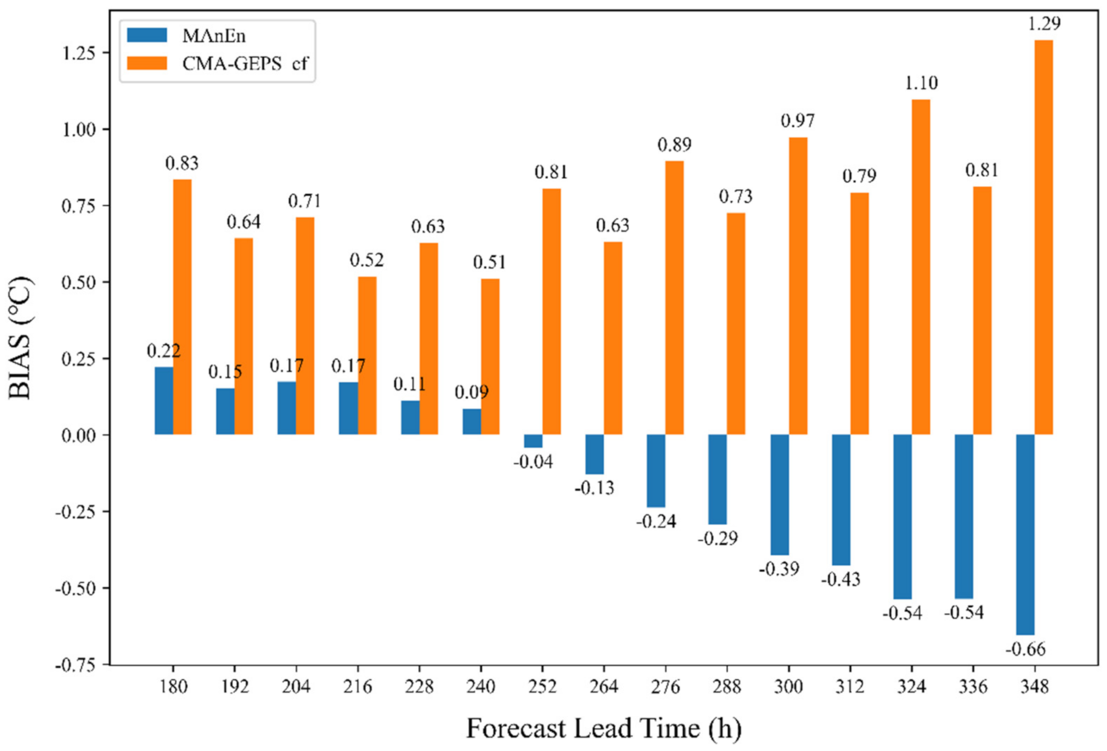
The bias corrections of 15 forecast periods of 180–348 h at 2405 stations in China were carried out using the analogue ensemble averaging forecast method. The bar chart of the bias of 2-m temperature model forecasts and analogue ensemble averaging forecasts from 1 May 2022, to 28 June 2022, are shown in Figure 2. It can be seen from the figure that the biases of the 2-m temperature model forecasts for the 15 forecast lead times are above 0.5 °C, and the largest bias is 1.29 °C. After correction, the biases are obviously reduced and the values are closer to 0. With the extension of forecast lead times, the biases gradually change from positive to negative and below 0.7 °C. In addition, the bias of the model forecasts for the adjacent forecast lead times is distributed in the high and low phases. This is because the 00 h model forecasts are better than the 12 h forecasts. In other words, the morning forecasts are better than the night forecasts.
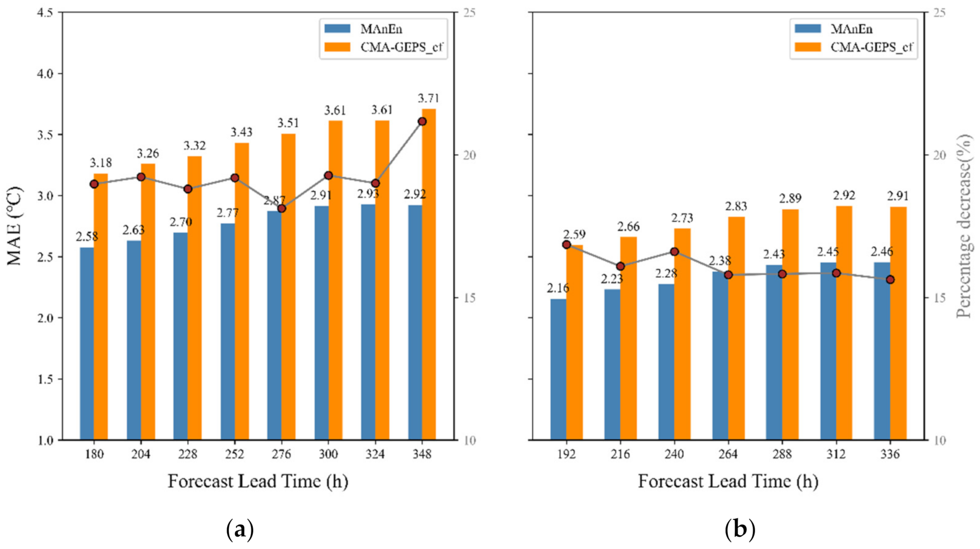
The MAE distributions for the analogue ensemble averaging forecasts and model forecasts under different forecast lead times at 2405 national stations are shown in Figure 3 (the mean of all stations with the same forecast lead time). After bias correction, the MAEs of all forecast lead times are reduced to below 3 °C, with decreases between 15% and 25 %. Figure 3a shows the MAEs of the daily 12 h forecasts for 7–14 days, and Figure 3b shows the MAEs of the daily 00 h forecasts. Comparing Figure 3a with Figure 3b, it can be seen that for the model forecasts, the daily 00 h forecast are always better than the 12 h forecasts. After bias correction is performed, using the analogue ensemble averaging method, the forecast gap between 00 h and 12 h forecasts improves.
The conclusions embodied in Figure 4 are similar to those in Figure 3, i.e., the RMSE and percentage decrease of the forecasts of 2-m temperature at 2405 national stations with forecast lead times of 180–348 h using the analogue ensemble averaging method and NWP model.
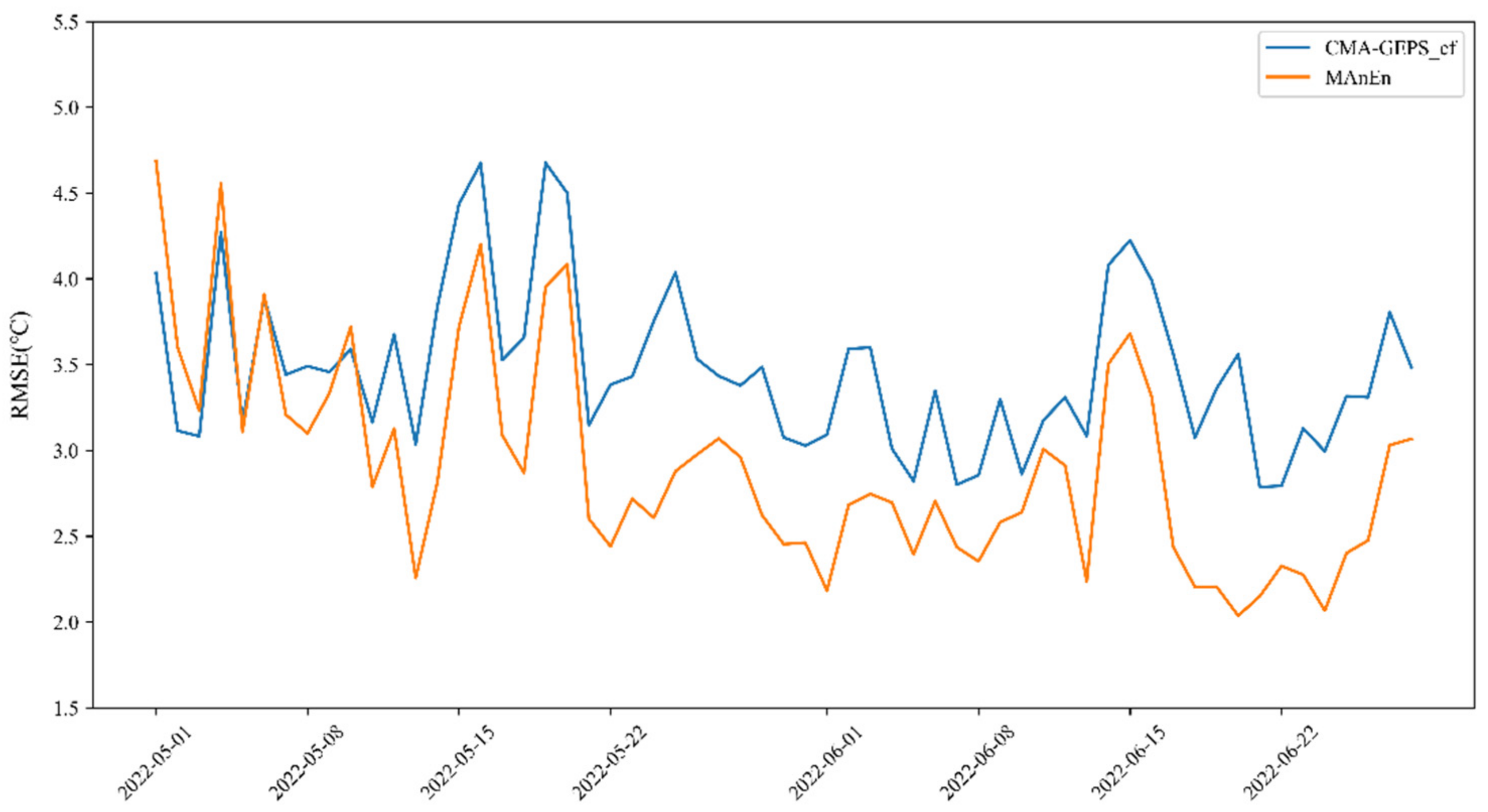
The analogue ensemble averaging method is used to test the 240 h forecasts of 2-m temperature for 2405 national stations from 1 May to 28 June 2022, and to examine the variation of the RMSE (Figure 5). As shown in Figure 5, the RMSE of the daily model forecast with a forecast lead time of 10 d is approximately 3.5 °C. After bias correction using the analogue ensemble averaging method, the RMSE is reduced to approximately 2.5 °C–3 °C, and the RMSE is reduced by 16% during the test dates.

4.2. Tests of Forecast Ability at the Stations

The RMSE distributions of the model forecasts and analogue ensemble averaging forecasts of 2405 stations with forecast times of 192 h, 240 h, 288 h, and 336 h from 1 May to 28 June 2022, are compared and analyzed, as shown in Figure 6.
It can be seen from the diagram that with the extension of the forecast lead times, the RMSE at the 2405 stations increase (comparing Figure 6a,c,e,g, and b,d,f,h, respectively), for both the model forecasts and the analogue ensemble averaging forecasts. The forecast difficulty of 2-m temperature gradually increases with the extension of the forecast lead times. For the same forecast lead time (comparing Figure 6a and b, c and d, e and f, g and h), the RMSE of the model forecasts are reduced for most stations, especially in Northwest, Southwest, and North China, when using the analogue ensemble averaging forecast method. The 8-d, 10-d, 12-d, and 14-d forecasts are greatly improved, and the rest of the region is also improved. For the four forecast lead times, the percentage of stations with reduced RMSE to all stations is shown in the following table (Table 2).
The RMSE (a, c, e, and g) of 2-m temperature forecasts by the model are obviously smaller in South China, Central China, and East China, than in other regions. This is greatly related to the amount of observation data and the difference in terrain height between the actual measurement and the topographic height at which the forecast is located. In general, the more distributed the stations are, the more abundant the observation data and the more accurate the model forecast. In addition, the temperature forecast error related to the terrain height difference is part of the systematic bias of the model forecast and can be corrected by statistical methods. Figure 7 shows the RMSE distribution for the 2-m temperature forecasts using the 240 h forecast lead time at each station. The terrain height of the observation stations is ordered from smallest to largest after the model forecast and bias correction using the analogue ensemble averaging method.
Figure 7 shows that the RMSEs for the 2-m temperature forecasts at stations with higher terrain height have an increasing trend compared with plain areas, and the errors are larger. This indicates that the temperature prediction error in the complex terrain area has greater uncertainty than that in the plain area. However, after bias correction using the analogue ensemble averaging forecast method, the RMSEs of the 2-m temperature forecasts of each station decrease, obviously, and a relatively consistent size is observed. This indicates that this method corrects the systematic error caused by the terrain height difference between the elevation of the station and the topographic height at which the forecast is located, and the correction effect is more significant for the stations with larger terrain heights.

4.3. Forecast Case

According to the above results, the analogue ensemble averaging method forecasts have better performance than the model forecasts, and the model forecast errors are effectively reduced.
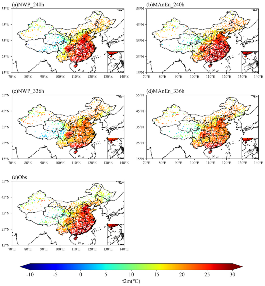
Figure 8 shows the results from the 240-h model forecasts results and analogue ensemble averaging method forecasts starting from 00 h on 5 June 2022, and the 336-h forecast results from 00 h on 22 May 2022. For both the 240-h and the 336-h 2-m temperature forecasts, the results after the correction of the analogue ensemble averaging method are closer to the actual observation than the model forecasts. From the overall regional point of view, after correction, the results from the Southwest, Central and North China are closer to the station observations.

5. Conclusions and Discussion

In this paper, the ‘analogue’ concept is applied to the statistical interpretation of the medium- and long-term forecasts of the model, and the analogue ensemble averaging correction method is developed. Based on the CMA-GEPS model, the 180–348 h forecasts of 2-m temperature and the observation data of 2405 stations in China are tested and analyzed, and compared with the model forecasts. The performance of the analogue ensemble averaging method is analyzed by several key test indexes, such as bias, MAE, and RMSE. The following conclusions are obtained:
(1)
The analogue ensemble averaging method has a good correction effect on the long forecast time of 180–348 h and effectively reduces the systematic error of the model forecasts of the 2-m temperature, which is higher at night and lower during the day. The forecast deviation is reduced by approximately 0.5 °C, and the MAE and RMSE are reduced by approximately 10–20%. During the test period from 1 May to 28 June 2022, the RMSE reduction rate of 240 h forecast reached 91% (the proportion of samples with reduced RMSE to all samples). Comparing the correction effect of different forecast lead times, the analogue ensemble averaging forecast method still has a better correction effect in longer forecast lead times.
(2)
After comparisons based on the spatial prediction results from 2405 stations, it is shown that the application of the analogue ensemble averaging forecast method effectively reduces the RMSEs of forecasts in Southwest China, Northwest China, and North China. The improvement rate of different forecast times reaches 31.4%. This method has a more obvious effect on the correction of complex terrain areas.
In this paper, only a factor of 2-m temperature is comprehensively tested and evaluated. In the future, multifactor application tests and evaluations need to be carried out. In addition, for the analogue ensemble averaging correction method, the length of the historical forecast dataset, the design of the similarity measure, the meteorological elements used in the selection of similar historical forecasts, and the forecast lead times are the key factors affecting the correction effect. Therefore, in the future, we will focus on the different forecast elements: (1) establish a longer historical forecast dataset so that there are more opportunities to find results similar to the current forecast; (2) for different forecast elements, more model predictors are used as similar reference factors, and the optimal weight combination is found to improve the correction effect; and (3) the actual data corresponding to the historical forecast selected by the analogue ensemble method can not only generate deterministic forecasts by averaging, but also generate probability forecasts, and can be used for objective correction of precipitation forecasts.

Author Contributions

Conceptualization, Y.H. and Q.W.; methodology, Y.H.; validation, Y.H.; formal analysis, Y.H.; investigation, Y.H.; resources, Q.W.; data curation, Y.H. and Q.W.; writing—original draft preparation, Y.H.; writing—review and editing, Q.W. and X.S.; visualization, Y.H.; supervision, Q.W. and X.S.; project administration, X.S.; funding acquisition, X.S. All authors have read and agreed to the published version of the manuscript.

Funding

This research was supported by grants from the NSFC Project (41975100).

Institutional Review Board Statement

Not applicable.

Informed Consent Statement

Not applicable.

Data Availability Statement

Restrictions apply to the availability of these data. Data was obtained from CMA and are available from the corresponding authors with the permission of CMA.

Acknowledgments

We acknowledge support from the above funding projects.

Conflicts of Interest

The authors declare no conflict of interest.

References

  1. Knag, Z.M.; Bao, Y.Y.; Zhou, N.F. Current Situation and Development of Medium-Range and Extended-Range Weather Forecast in China. Adv. Meteor. Sci. Technol. 2013, 3, 18–24. [Google Scholar]
  2. Zhang, J.J.; Ge, L. Basis of Medium-and Long-Term Weather Forecast, 1st ed.; China Meteorological Press: Beijing, China, 1983.
  3. Lorenz, E.N. Deterministic Nonperiodic Flow. J. Atmos. Sci. 1963, 20, 130–141. [Google Scholar] [CrossRef]
  4. Bauer, P.; Thorpe, A.; Brunet, G. The quiet revolution of numerical weather prediction. Nature 2015, 525, 47–55. [Google Scholar] [CrossRef] [PubMed]
  5. Chen, D.H.; Xue, J.S. An overview on recent progresses of the operational numerical weather prediction models. Acta Meteor. Sin. 2004, 62, 623–633. [Google Scholar]
  6. Dai, K.; Cao, Y.; Qian, Q.F.; Gao, S.; Zhao, S.G.; Chen, Y.; Qian, C.H. Situation and Tendency of Operational Technologies in Short-and Medium-Range Weather Forecast. Meteor. Mon 2016, 42, 1445–1455. [Google Scholar]
  7. Li, Z.C.; Bi, B.G.; Jin, R.H.; Xu, Z.F.; Xue, F. The development and application of the modern weather forecast in China for the recent 10 years. Acta Meteor. Sin. 2014, 72, 1069–1078. [Google Scholar]
  8. Shen, X.S.; Wang, J.J.; Li, Z.C.; Chen, D.H.; Gong, J.D. China’s independent and innovative development of numerical weather prediction. Acta Meteor. Sin. 2020, 78, 451–476. [Google Scholar]
  9. Sun, C.; Liang, X. Understanding and Reducing Warm and Dry Summer Biases in the Central United States: Analytical Modeling to Identify the Mechanisms for CMIP Ensemble Error Spread. J. Clim. 2022, 1–42. [Google Scholar] [CrossRef]
  10. Sun, C.; Liang, X. Understanding and Reducing Warm and Dry Summer Biases in the Central United States: Improving Cumulus Parameterization. J. Clim. 2022, 1–42. [Google Scholar] [CrossRef]
  11. Bannister, R.N. A review of operational methods of variational and ensemble-variational data assimilation. Quart. J. Roy Meteor. Soc. 2017, 143, 607–633. [Google Scholar] [CrossRef] [Green Version]
  12. Tao, Z.Y.; Zhao, C.G.; Chen, M. The Necessity of Statistical Forecasts. Adv. Meteor. Sci. Technol. 2016, 6, 6–13. [Google Scholar]
  13. Su, X.; Yuan, H.L. The research progress of ensemble statistical postprocessing methods. Adv. Meteor. Sci. Technol. 2020, 10, 30–41. [Google Scholar]
  14. Klein, W.H.; Lewis, B.M.; Enger, I. Objective prediction of five-day mean temperature during winter. J. Meteorol. 1959, 16, 672–682. [Google Scholar] [CrossRef]
  15. Carter, G.M.; Dallavalle, J.P.; Glahn, H.R. Statistical forecasts based on the National Meteorological Center’s numerical weather prediction system. Weather. Forecast. 1989, 4, 401–412. [Google Scholar] [CrossRef]
  16. Glahn, H.R.; Lowry, D.A. The use of Model Output Statistics (MOS) in objective weather forecasting. J. Appl. Meteorol. 1972, 11, 1203–1211. [Google Scholar] [CrossRef]
  17. Ding, S.S. The advance of model output statistics method in China. Acta Meteor Sin. 1985, 43, 332–338. [Google Scholar]
  18. Lemcke, C.; Kruizinga, S. Model output statistics forecasts: Three years of operational experience in the Netherlands. Mon. Weather. Rev. 1988, 116, 1077–1090. [Google Scholar] [CrossRef]
  19. Francis, P.E.; Day, A.P.; Davis, G.P. Automated temperature forecasting, an application of Model Output Statistics to the Meteorological Office numerical weather prediction model. Meteorol. Mag. 1982, 111, 73–87. [Google Scholar]
  20. Conte, M.; DeSimone, C.; Finizio, C. Post-processing of numerical models: Forecasting the maximum temperature at Milano Linate. Rev. Meteor. Aeronautica. 1980, 40, 247–265. [Google Scholar]
  21. Lu, R. The application of NWP products and progress of interpretation techniques in China. In Programme on Short- and Medium-Range Weather Prediction Research; Glahn, H.R., Murphy, A.H., Wilson, L.J., Jensenius, J.S., Jr., Eds.; World Meteorological Organization: Geneva, Switzerland, 1991; pp. 19–22. [Google Scholar]
  22. Azcarraga, R.; Ballester, G.A.J. Statistical system for forecasting in Spain. In Programme on Short- and Medium-Range Weather Prediction Research; Glahn, H.R., Murphy, A.H., Wilson, L.J., Jensenius, J.S., Jr., Eds.; World Meteorological Organization: Geneva, Switzerland, 1991; pp. 23–25. [Google Scholar]
  23. Brunet, N.; Verret, R.; Yacowar, N. An objective comparison of model output statistics and “perfect prog” systems in producing numerical weather element forecasts. Weather. Forecast. 1988, 3, 273–283. [Google Scholar] [CrossRef]
  24. Lu, R.H.; Xu, C.Y.; Zhang, L.; Mao, W.X. Calculation method for initial value of Kalman Filter and its application. Quart. J. Appl. Meteor. 1997, 8, 34–43. [Google Scholar]
  25. Homleid, M. Diurnal corrections of short-term surface temperature forecasts using Kalman filter. Wea. Forecast. 1995, 10, 689–707. [Google Scholar] [CrossRef]
  26. Galanis, G.; Anadranistakis, M. A one-dimensional Kalman filter for the correction of near surface temperature forecasts. Meteorol. Appl. 2002, 9, 437–441. [Google Scholar] [CrossRef] [Green Version]
  27. Liu, S.Y.; Xu, L.Q.; Li, D.L. Multi-scale prediction of water temperature using empirical mode decomposition with back-propagation neural networks. Comput. Electr. Eng. 2016, 49, 1–8. [Google Scholar] [CrossRef]
  28. Xiong, S.W.; Yu, L.H.; Hu, S.S.; Shen, A.Y.; Shen, Y.; Jing, Y.S. An optimized BP-MOS temperature forecast method based on the fine-mesh products of ECMWF. J. Arid. Meteorol. 2017, 35, 668–673. [Google Scholar]
  29. Feng, H.Z.; Chen, Y.Y. Application of support vector machine regression method in weather forecast. Meteor. Mon. 2005, 31, 41–44. [Google Scholar]
  30. Sun, J.; Cao, Z.; Li, H.; Qian, S.; Wang, X.; Yan, L.; Xue, W. Application of artificial intelligence technology to numerical weather prediction. J. Appl. Meteor. Sci. 2021, 32, 1–11. [Google Scholar]
  31. Han, L.; Chen, M.; Chen, K.; Chen, H.; Zhang, Y.; Lu, B.; Song, L.; Qin, R. A deep learning method for bias correction of ECMWF 24–240 h forecasts. Adv. Atmos. Sci. 2021, 38, 1444–1459. [Google Scholar] [CrossRef]
  32. Peng, T.; Zhi, X.F.; Ji, Y.; Ji, L.Y.; Ye, T. Prediction skill of extended range 2 m maximum air temperature probabilistic forecasts using machine learning Post-processing methods. Atmosphere 2020, 11, 823. [Google Scholar] [CrossRef]
  33. Zarei, M.; Najarchi, M.; Mastouri, R. Bias correction of global ensemble precipitation forecasts by Random Forest method. Earth Sci. Inform. 2021, 14, 677–689. [Google Scholar] [CrossRef]
  34. Zhang, H.; Wang, Y.; Chen, D.; Feng, D.; You, X.; Wu, W. Temperature Forecasting Correction Based on Operational GRAPES-3km Model Using Machine Learning Methods. Atmosphere 2022, 13, 362. [Google Scholar] [CrossRef]
  35. Hamill, T.M.; Whitaker, J.S. Probabilistic quantitative precipitation forecasts based on reforecast analogs: Theory and application. Mon. Weather. Rev. 2006, 134, 3209–3229. [Google Scholar] [CrossRef]
  36. Mayr, G.J.; Messner, J.W. Probabilistic Forecasts Using Analogs in the Idealized Lorenz96 Setting. Mon. Weather. Rev. 2011, 139, 1960–1971. [Google Scholar]
  37. Delle Monache, L.; Eckel, F.A.; Rife, D.L.; Nagarajan, B.; Searight, K. Probabilistic Weather Prediction with an Analog Ensemble. Mon. Weather. Rev. 2013, 141, 3498–3516. [Google Scholar] [CrossRef] [Green Version]
  38. Junk, C.; Monache, L.D.; Alessandrini, S.; Cervone, G.; Von Bremen, L. Predictor-weighting strategies for probabilistic wind power forecasting with an analog ensemble. Meteorol. Z. 2015, 24, 361–379. [Google Scholar] [CrossRef]
  39. Yang, J.; Astitha, M.; Monache, L.D.; Alessandrini, S. An analog technique to improve storm wind speed prediction using a dual NWP model approach. Mon. Weather. Rev. 2018, 146, 4057–4077. [Google Scholar] [CrossRef]
  40. Alessandrini, S.; Delle Monache, L.; Sperati, S.; Nissen, J. A novel application of an analog ensemble for short-term wind power forecasting. Renew. Energy 2015, 76, 768–781. [Google Scholar] [CrossRef]
  41. Monache, L.D.; Nipen, T.; Liu, Y.; Roux, G.; Stull, R.B. Kalman filter and analog schemes to postprocess numerical weather predictions. Mon. Weather. Rev. 2011, 139, 3554–3570. [Google Scholar] [CrossRef] [Green Version]
  42. Mahoney, W.P.; Parks, K.; Wiener, G.; Liu, Y.; Myers, W.L.; Sun, J.; Monache, L.D.; Hopson, T.; Johnson, D.; Haupt, S.E. A wind power forecasting system to optimize grid integration. IEEE Trans. Sustain. Energy 2012, 3, 670–682. [Google Scholar] [CrossRef]
  43. Eckel, F.A.; Delle Monache, L. A hybrid NWP-analog ensemble. Mon. Weather. Rev. 2016, 144, 897–911. [Google Scholar] [CrossRef]
  44. Hamill, T.M.; Scheuerer, M.; Bates, G.T. Analog Probabilistic Precipitation Forecasts Using GEFS Reforecasts and Climatology-Calibrated Precipitation Analyses*. Mon. Weather. Rev. 2015, 143, 3300–3309. [Google Scholar] [CrossRef] [Green Version]
  45. Panziera, L.; Germann, U.; Gabella, M.; Mandapaka, P.V. NORA–Nowcasting of orographic rainfall by means of an alogues. Quart. J. Roy. Meteor. Soc. 2011, 137, 2106–2123. [Google Scholar] [CrossRef]
  46. Liu, C.X. The short-term climate forecasting of tropical cyclone in Guangdong: In the phase space similarity method. J. Trop. Meteor. 2002, 18, 83–90. [Google Scholar]
  47. Alessandrini, S.; Monache, L.D.; Rozoff, C.M.; Lewis, W.E. Probabilistic Prediction of Tropical Cyclone Intensity with an Analog Ensemble. Mon. Weather. Rev. 2018, 146, 1723–1744. [Google Scholar] [CrossRef]
  48. Chen, P.; Yu, H.; Brown, B.; Chen, G.; Wan, R. A probabilistic climatology-based analogue intensity forecast scheme for tropical cyclones. Q. J. R. Meteorol. Soc. 2016, 142, 2386–2397. [Google Scholar] [CrossRef]
  49. Djalalova, I.; Monache, L.D.; Wilczak, J. PM2.5 analog forecast and Kalman filter post-processing for the Community Multiscale Air Quality (CMAQ) model. Atmos. Environ. 2015, 108, 76–87. [Google Scholar] [CrossRef]
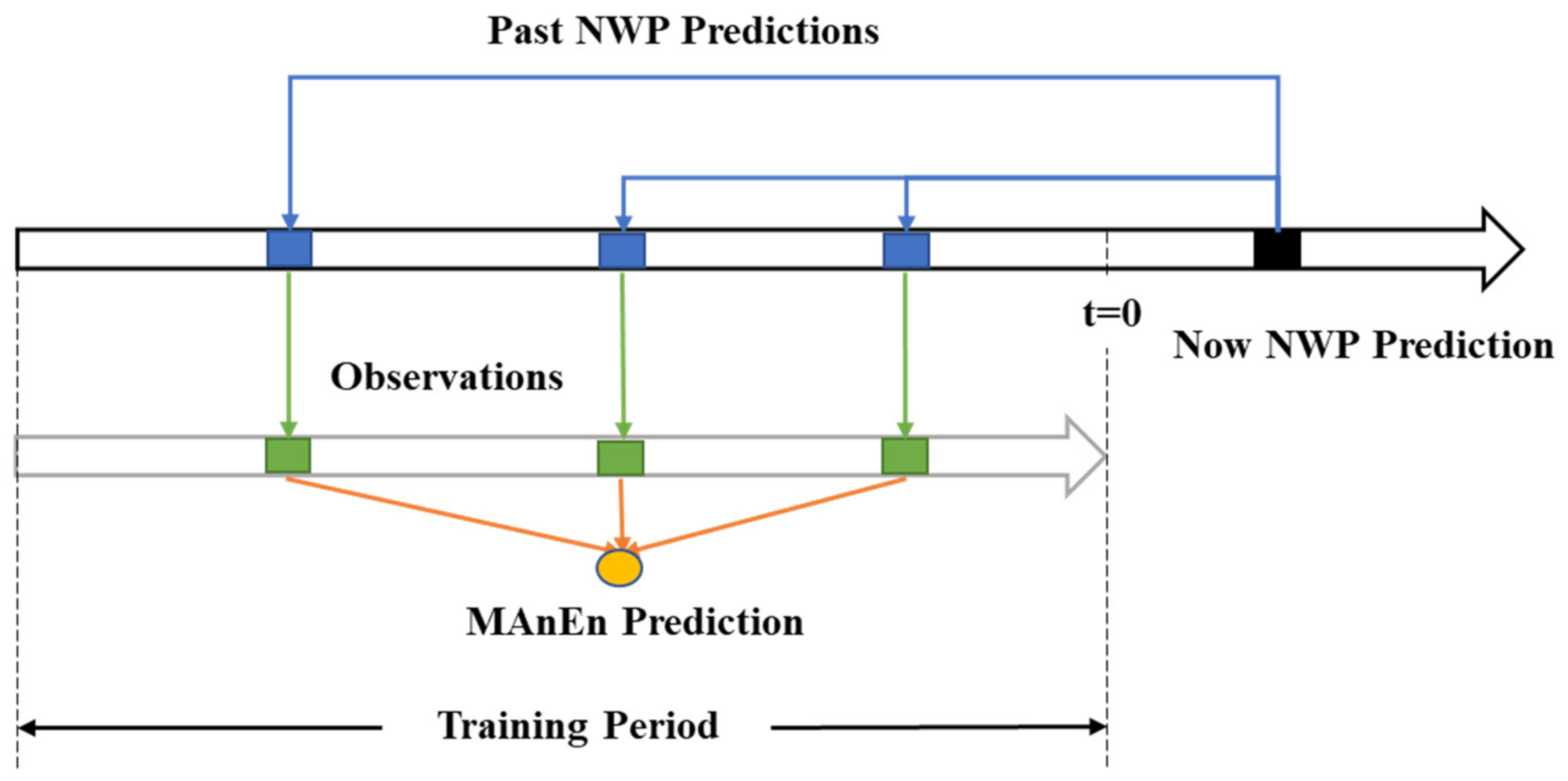
Figure 1. Flow chart of the analogue ensemble averaging method (MAnEn).
Atmosphere 13 02097 g001
Figure 2. The biases of 2-m temperature between analogue ensemble averaging forecasts and model forecasts for the forecast lead times of 180–348 h.
Atmosphere 13 02097 g002
Figure 3. MAE and percentage decrease of analog ensemble averaging forecasts and model forecasts. (a) Daily 12 h forecasts for 7–14 d; (b) daily 00 h forecasts for 8–14 d.
Atmosphere 13 02097 g003
Figure 4. RMSE and percentage decrease of the analog ensemble averaging forecasts and model forecasts. (a) Daily 12 h forecast for 7–14 d; (b) daily 00 h forecast for 8–14 d.
Atmosphere 13 02097 g004
Figure 5. RMSE of daily 240 h forecast for 1 May–28 June 2022.
Atmosphere 13 02097 g005
Figure 6. RMSE distribution of model forecasts and analog ensemble averaging forecasts for 2405 stations. ((a,c,e,g) are model forecasts; (b,d,f,h) are analog ensemble averaging forecasts).
Atmosphere 13 02097 g006
Figure 7. RMSE of model forecasts and analog ensemble averaging forecasts and the terrain height of stations.
Atmosphere 13 02097 g007
Figure 8. Observations, 240-h, and-336 h model forecasts, the analogue ensemble averaging forecasts of 2-m temperature ((a,c): model forecasts; (b,d): analogue ensemble mean forecasts; (e): observations) at 00:00 UTC on 5 June 2022.
Atmosphere 13 02097 g008
Table 1. Data duration and parameter setting for each forecast time.
Forecast Lead TimeTesting PeriodTraining PeriodSelected Lead TimeAnalog Ensemble Members
180 h20220501–0628
(59 d)
20181225–20220423 (1216 d)168 h, 180 h, 192 h30
192 h–20220422 (1215 d)180 h, 192 h, 204 h
204 h1215 d192 h, 204 h, 216 h
216 h–20220421 (1214 d)204 h, 216 h, 228 h
228 h1214 d216 h, 228 h, 240 h
240 h–20220420 (1213 d)228 h, 240 h, 252 h
252 h1213 d240 h, 252 h, 264 h
264 h–20220419 (1212 d)252 h, 264 h, 276 h
276 h1212 d264 h, 276 h, 288 h
288 h–20220418 (1211 d)276 h, 288 h, 300 h
300 h1211 d288 h, 300 h, 312 h
312 h–20220417 (1210 d)300 h, 312 h, 324 h
324 h1210 d312 h, 324 h, 336 h
336 h–20220416 (1209 d)324 h, 336 h, 348 h
348 h1209 d336 h, 348 h, 360 h
Table 2. The decreasing percent of RMSE of the stations.
Forecast Lead TimeDecreasing Percent
192 h31.4%
240 h29.6%
288 h23.5%
336 h24.4%
Publisher’s Note: MDPI stays neutral with regard to jurisdictional claims in published maps and institutional affiliations.