
Analysis of the Spatial–Temporal Distribution Characteristics of NO2 and Their Influencing Factors in the Yangtze River Delta Based on Sentinel-5P Satellite Data
 ,
,
Abstract
1. Introduction
2. Materials and Methods
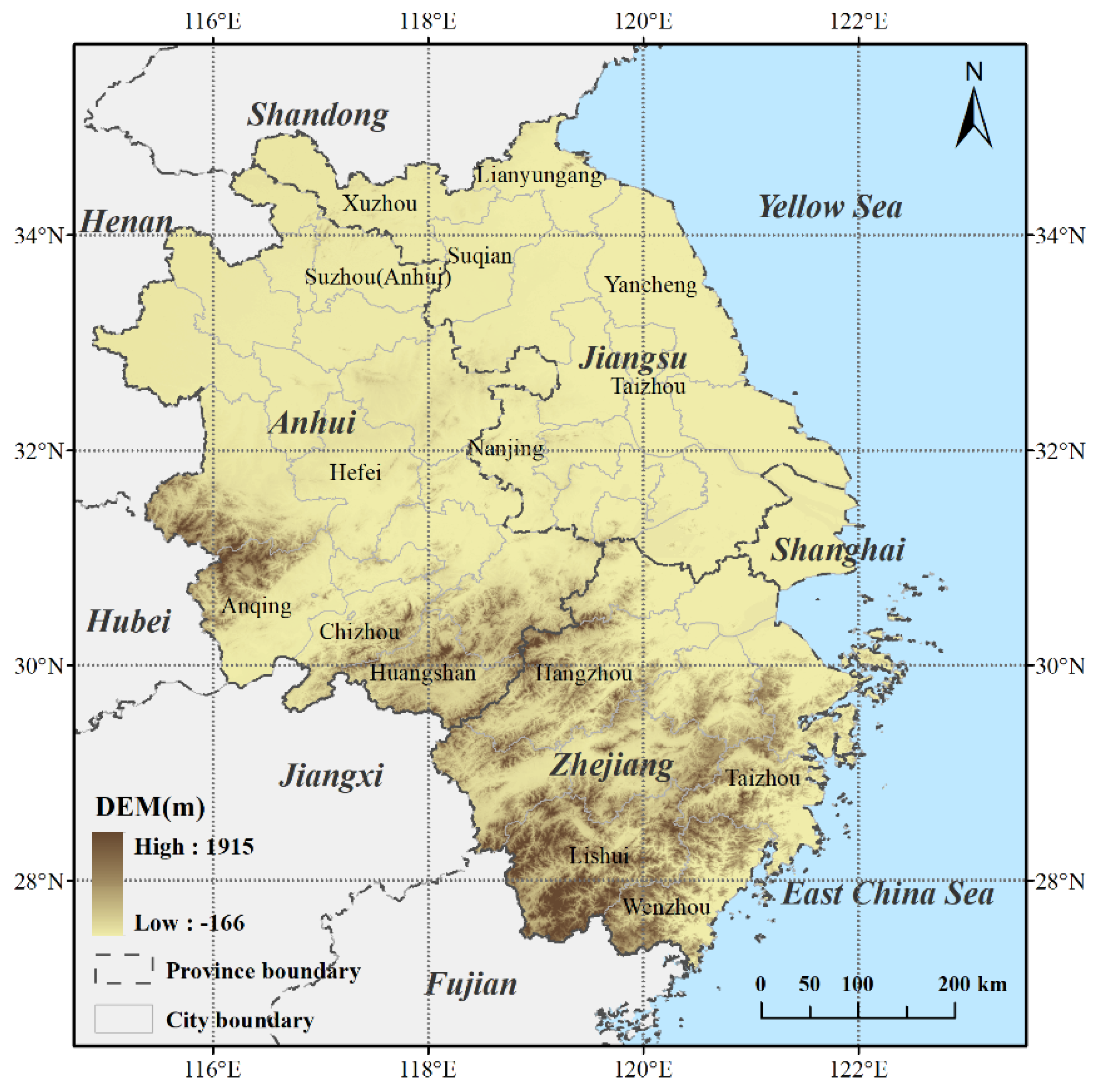
2.1. Study Area
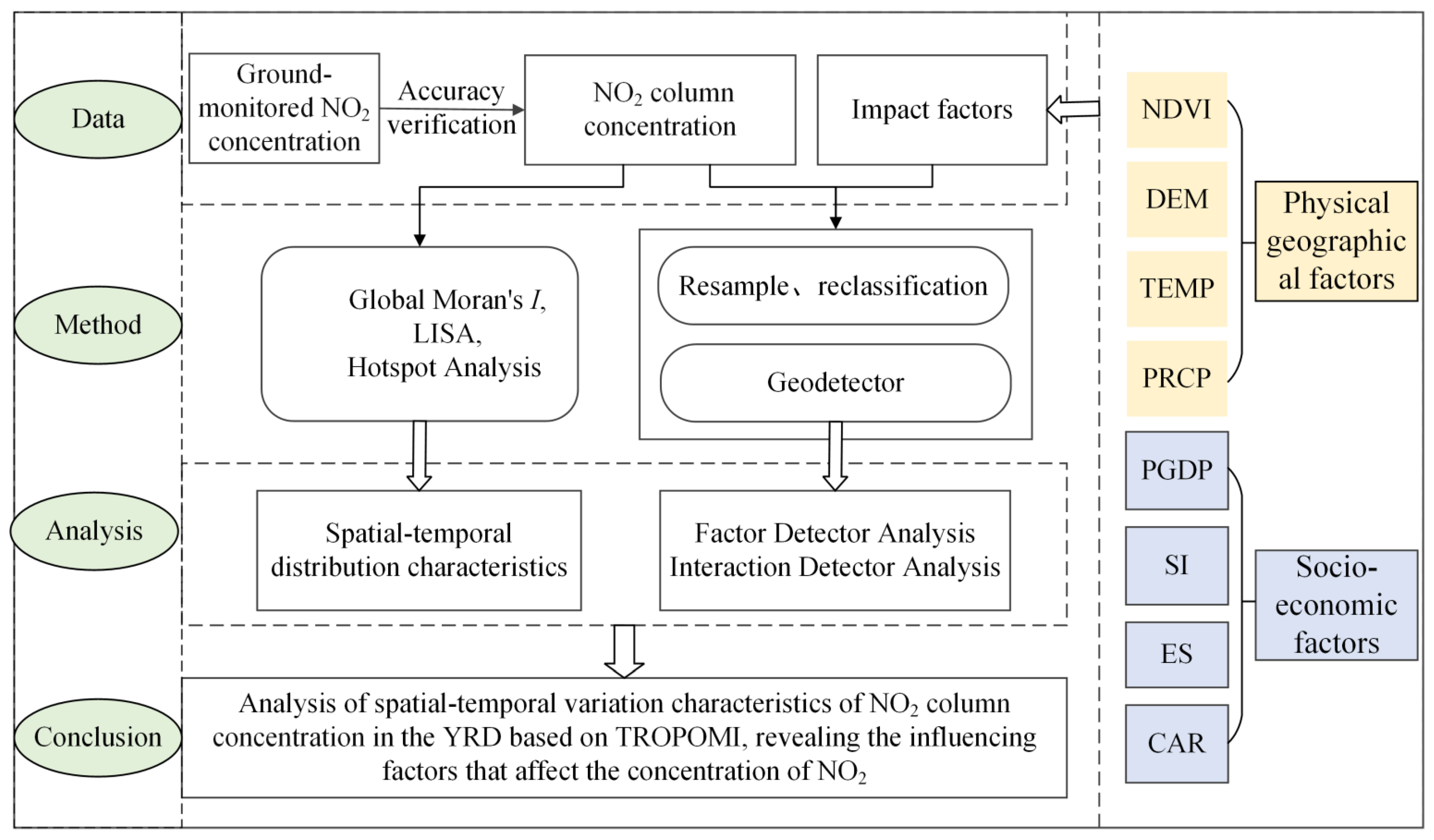
2.2. Data Sources
2.3. Methods
2.3.1. Spatial Autocorrelation Analysis
2.3.2. Hotspot Analysis
2.3.3. Geodetector
3. Results
3.1. Comparison and Verification between the NO2 Column Concentration and the Ground-Monitored NO2 Concentrations
3.2. Spatial–Temporal Distribution Characteristics of the NO2 Column Concentration
3.2.1. Temporal Distribution Characteristics of the NO2 Column Concentration in the YRD
3.2.2. Spatial Distribution Characteristics of NO2 Column Concentration in the YRD
3.3. Spatial Agglomeration Characteristics of the NO2 Column Concentration in the YRD
3.4. Influencing Factor Analysis of NO2 Column Concentration Distribution in the YRD
3.4.1. Factor Detector Analysis
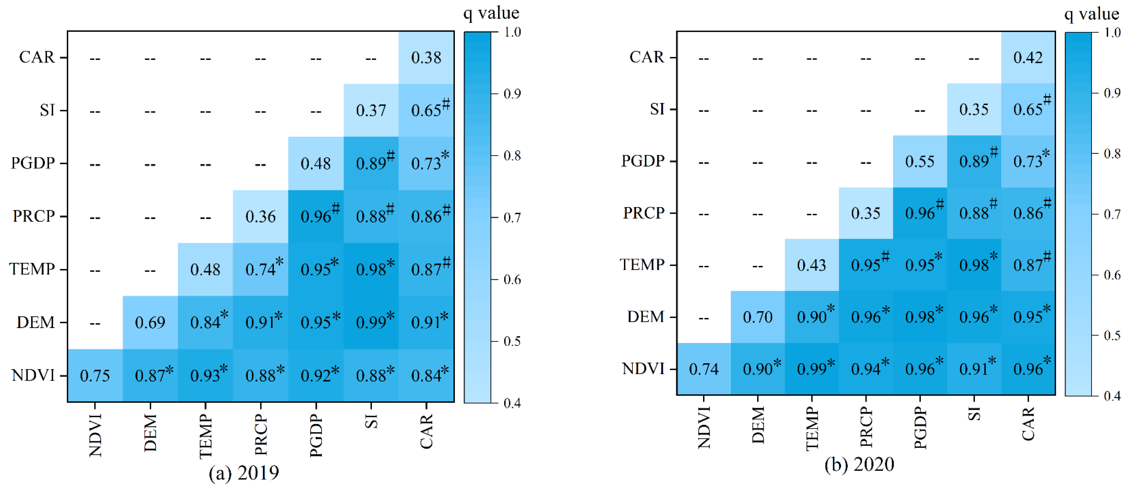
3.4.2. Interaction Detector Analysis
4. Discussion
4.1. Spatial–Temporal Distribution Characteristics of NO2 Column Concentration
4.2. Influencing Factors of NO2 Column Concentration
4.2.1. Physical Geographical Factors
4.2.2. Socio-Economic Factors
4.3. Strengths and Limitations of this Study
5. Conclusions
- (1)
- Based on the ground-monitored NO2 concentration data, the correlation tests showed that the NO2 column concentration observed by TROPOMI could reflect the real NO2 pollution scenario on the surface.
- (2)
- The annual variation trend of NO2 column concentrations in the YRD region from 2019 to 2020 exhibited a ‘U’-shaped curve, and there was a seasonal characteristic of ‘high in winter and low in summer’. In terms of the spatial distribution, the NO2 column concentration in the YRD was the highest in the central region and the lowest in high-altitude areas in the south and the coastal area in the northeast.
- (3)
- The factor detection results show that the influences of vegetation and altitude were the largest. Further, by comparing the influences of various factors in 2019 and 2020, it was found that economic development and traffic had a greater impact on the concentrations of NO2.
Author Contributions
Funding
Institutional Review Board Statement
Informed Consent Statement
Data Availability Statement
Acknowledgments
Conflicts of Interest
References
- Cui, Y.; Wang, L.; Jiang, L.; Liu, M.; Wang, J.; Shi, K.; Duan, X. Dynamic spatial analysis of NO2 pollution over China: Satellite observations and spatial convergence models. Atmos. Pollut. Res. 2021, 12, 89–99. [Google Scholar] [CrossRef]
- Zhang, X.; Zhang, P.; Zhang, Y.; Li, X.; Qiu, H. The trend, seasonal cycle, and sources of tropospheric NO2 over China during 1997–2006 based on satellite measurement. Sci. China Ser. D Earth Sci. 2007, 50, 1877–1884. [Google Scholar] [CrossRef]
- Chen, R.; Huang, W.; Wong, C.-M.; Wang, Z.; Quoc Thach, T.; Chen, B.; Kan, H. Short-term exposure to sulfur dioxide and daily mortality in 17 Chinese cities: The China air pollution and health effects study (CAPES). Environ. Res. 2012, 118, 101–106. [Google Scholar] [CrossRef] [PubMed]
- Cui, Y.; Zhang, W.; Bao, H.; Wang, C.; Cai, W.; Yu, J.; Streets, D.G. Spatiotemporal dynamics of nitrogen dioxide pollution and urban development: Satellite observations over China, 2005–2016. Resour. Conserv. Recycl. 2019, 142, 59–68. [Google Scholar] [CrossRef]
- Xu, Y.; Wang, D.; Wu, Z. Spatio-temporal Variations of Troposhperic NO2 over China in 1996–2010 based on Remote Sensing Data. Remote Sens. Technol. Appl. 2013, 28, 898–903. (In Chinese) [Google Scholar]
- Richter, A.; Burrows, J.P. Tropospheric NO2 from GOME measurements. Adv. Space Res. 2002, 29, 1673–1683. [Google Scholar] [CrossRef]
- Piters, A.; Bramstedt, K.; Lambert, J.-C.; Kirchhoff, B.J.A.C. Overview of SCIAMACHY validation: 2002–2004. Atmos. Chem. Phys. 2006, 6, 127–148. [Google Scholar] [CrossRef]
- Boersma, K.F.; Jacob, D.J.; Eskes, H.J.; Pinder, R.W.; Wang, J.; Van Der A, R.J. Intercomparison of SCIAMACHY and OMI tropospheric NO2 columns: Observing the diurnal evolution of chemistry and emissions from space. J. Geophys. Res. 2008, 113, D16S26. [Google Scholar]
- Van Geffen, J.; Eskes, H.; Compernolle, S.; Pinardi, G.; Verhoelst, T.; Lambert, J.C.; Sneep, M.; ter Linden, M.; Ludewig, A.; Boersma, K.F.; et al. Sentinel-5P TROPOMI NO2 retrieval: Impact of version V2.2 improvements and comparisons with OMI and ground-based data. Atmos. Meas. Tech. 2022, 15, 2037–2060. [Google Scholar] [CrossRef]
- Berger, M.; Moreno, J.; Johannessen, J.A.; Levelt, P.F.; Hanssen, R.F. ESA’s sentinel missions in support of Earth system science. Remote Sens. Environ. 2012, 120, 84–90. [Google Scholar] [CrossRef]
- Guanter, L.; Aben, I.; Tol, P.; Krijger, J.M.; Hollstein, A.; Köhler, P.; Damm, A.; Joiner, J.; Frankenberg, C.; Landgraf, J. Potential of the TROPOspheric Monitoring Instrument (TROPOMI) onboard the Sentinel-5 Precursor for the monitoring of terrestrial chlorophyll fluorescence. Atmos. Meas. Tech. 2015, 8, 1337–1352. [Google Scholar] [CrossRef]
- Liu, H.F.C.; Huang, J.; Zhu, X.; Zhou, Y.; Wang, Z.; Zhang, Q. The spatial-temporal characteristics and influencing factors of air pollution in Beijing-Tianjin-Hebei urban agglomerration. Acta Ecol. Sin. 2018, 73, 177–191. (In Chinese) [Google Scholar]
- Zheng, Z.; Yang, Z.; Wu, Z.; Marinello, F. Spatial Variation of NO2 and Its Impact Factors in China: An Application of Sentinel-5P Products. Remote Sens. 2019, 11, 1939. [Google Scholar] [CrossRef]
- Judd, L.M.; Al-Saadi, J.A.; Szykman, J.J.; Valin, L.C.; Janz, S.J.; Kowalewski, M.G.; Eskes, H.J.; Veefkind, J.P.; Cede, A.; Mueller, M.; et al. Evaluating Sentinel-5P TROPOMI tropospheric NO2 column densities with airborne and Pandora spectrometers near New York City and Long Island Sound. Atmos. Meas. Tech. 2020, 13, 6113–6140. [Google Scholar] [CrossRef] [PubMed]
- Ghasempour, F.; Sekertekin, A.; Kutoglu, S.H. Google Earth Engine based spatio-temporal analysis of air pollutants before and during the first wave COVID-19 outbreak over Turkey via remote sensing. J. Clean. Prod. 2021, 319, 128599. [Google Scholar] [CrossRef] [PubMed]
- Schneider, P.; Hamer, P.D.; Kylling, A.; Shetty, S.; Stebel, K. Spatiotemporal Patterns in Data Availability of the Sentinel-5P NO2 Product over Urban Areas in Norway. Remote Sens. 2021, 13, 2095. [Google Scholar] [CrossRef]
- Zheng, Z.W.Z.; Chen, Y.; Yang, Z.; Marinello, F. Analysis of temporal and spatial variation characteristics of NO2 pollutants in Guangdong-Hong Kong-Macao Greater Bay Area based on Sentinel-5P satellite data. China Environ. Sci. 2021, 41, 63–72. [Google Scholar]
- Wang, J.Y.J.; Guo, H.; Wang, X.; Liu, B.; Li, Y. Spatio-temporal analysis of NO2 column density in Beijing-Tianjin-Hebei region based on TROPOMI. Environ. Sci. Technol. 2022, 45, 21–31. (In Chinese) [Google Scholar]
- He, J.; Hu, S. Ecological efficiency and its determining factors in an urban agglomeration in China: The Chengdu-Chongqing urban agglomeration. Urban Clim. 2022, 41, 101071. [Google Scholar] [CrossRef]
- Lei, Y.; Zhao, J. Development track and new-type urbanization apporoaches in major conurbation in China. Acta Sci. Nat. Univ. Sunyatseni 2016, 55, 141–150. (In Chinese) [Google Scholar]
- The Central Committee of the Communist Party of China and the State Council issued the “Outline of the Yangtze River Delta Regional Integrated Development Plan”. Available online: http://www.mofcom.gov.cn/article/b/g/202001/20200102931567.shtml (accessed on 18 August 2022).
- Xiao, Z.; Xie, X.; Chen, Y.; Liu, S.; Lin, X.; Chen, G. Temporal and spatial characteristics and influencing factors of NO2 pollution over Guangdong-Hong Kong-Macao Greater Bay Area. China Environ. Sci. 2020, 40, 2010–2017. [Google Scholar]
- Li, R.; Wang, Z.; Cui, L.; Fu, H.; Zhang, L.; Kong, L.; Chen, W.; Chen, J. Air pollution characteristics in China during 2015–2016: Spatiotemporal variations and key meteorological factors. Sci. Total Environ. 2019, 648, 902–915. [Google Scholar] [CrossRef] [PubMed]
- Wang, J.X.C. Geodetector: Principle and prospective. Acta Ecol. Sin. 2017, 72, 116–134. (In Chinese) [Google Scholar]
- Han, K.M. Temporal Analysis of OMI-Observed Tropospheric NO2 Columns over East Asia during 2006–2015. Atmosphere 2019, 10, 658. [Google Scholar] [CrossRef]
- Boersma, K.F.; Eskes, H.J.; Dirksen, R.J.; van der A, R.J.; Veefkind, J.P.; Stammes, P.; Huijnen, V.; Kleipool, Q.L.; Sneep, M.; Claas, J.; et al. An improved tropospheric NO2 column retrieval algorithm for the Ozone Monitoring Instrument. Atmos. Meas. Tech. 2011, 4, 1905–1928. [Google Scholar] [CrossRef]
- Boersma, K.F.; Eskes, H.J.; Veefkind, J.P.; Brinksma, E.J.; van der A, R.J.; Sneep, M.; van den Oord, G.H.J.; Levelt, P.F.; Stammes, P.; Gleason, J.F.; et al. Near-real time retrieval of tropospheric NO2 from OMI. Atmos. Chem. Phys. 2007, 7, 2103–2118. [Google Scholar] [CrossRef]
- United States Geological Survey (USGS). Available online: https://lpdaac.usgs.gov/node/838 (accessed on 19 August 2022).
- Farr, T.G.; Rosen, P.A.; Caro, E.; Crippen, R.; Duren, R.; Hensley, S.; Kobrick, M.; Paller, M.; Rodriguez, E.; Roth, L.; et al. The Shuttle Radar Topography Mission. Rev. Geophys. 2007, 45, RG2004. [Google Scholar] [CrossRef]
- Li, H.; Zhang, J.; Wen, B.; Huang, S.; Gao, S.; Li, H.; Zhao, Z.; Zhang, Y.; Fu, G.; Bai, J.; et al. Spatial-Temporal Distribution and Variation of NO2 and Its Sources and Chemical Sinks in Shanxi Province, China. Atmosphere 2022, 13, 1096. [Google Scholar] [CrossRef]
- He, Y.; Lin, K.; Liao, N.; Chen, Z.; Rao, J. Exploring the spatial effects and influencing factors of PM2.5 concentration in the Yangtze River Delta Urban Agglomerations of China. Atmos. Environ. 2022, 268, 118805. [Google Scholar] [CrossRef]
- Sokal, R.R.; Oden, N.L. Spatial autocorrelation in biology: 1. Methodology 1978, 10, 199–228. [Google Scholar]
- Moran, P.A.P. The interpretation of statistical maps. J. R. Stat. Soc. Ser B (Methodol.) 1948, 10, 243–251. [Google Scholar] [CrossRef]
- Anselin, L. Local indicators of spatial association-LISA. Geogr. Anal. 2010, 27, 93–115. [Google Scholar] [CrossRef]
- Wang, A.; Kang, P.; Zhang, Y.; Zeng, S.; Zhang, X.; Shi, J.; Liu, Z.; Xiang, Z.; Wang, K.; Zhang, S.; et al. Spatial differentiation and driving factors of aerosol optical depth in Sichuan Basin from 2003 to 2018. China Environ. Sci. 2022, 42, 528–538. (In Chinese) [Google Scholar]
- Zhang, Y.; Wang, L.; Tang, Z.; Zhang, K.; Wang, T. Spatial effects of urban expansion on air pollution and eco-efficiency: Evidence from multisource remote sensing and statistical data in China. J. Clean. Prod. 2022, 367, 132973. [Google Scholar] [CrossRef]
- Zhou, L.; Wu, J.; Jia, R.; Liang, N.; Zhang, F.; Ni, Y.; Liu, M. Investigation of temporal-spatial characteristics and underlying risk factors of PM2.5 pollution in Beijing-Tianjin- Hebei Area. Res. Environ. Sci. 2016, 29, 483–493. [Google Scholar]
- Liu, X.; Yi, G.; Zhou, X.; Zhang, T.; Lan, Y.; Yu, D.; Wen, B.; Hu, J. Atmospheric NO2 Distribution Characteristics and Influencing Factors in Yangtze River Economic Belt: Analysis of the NO2 Product of TROPOMI/Sentinel-5P. Atmosphere 2021, 12, 1142. [Google Scholar] [CrossRef]
- Liu, Y.; Xie, Y. Remote sensing monitoring of NO2 concentration based on Sentinel-5P in China. China Environ. Sci. 2022, 42, 1–16. (In Chinese) [Google Scholar]
- Yu, L.; He, W.; Li, N.; Lu, J.; Xie, S.; Huang, L. Analysis of temporal and spatial variation characteristics and influencing factors of NO2 pollutants in Guangxi. Environ. Sci. Technol. 2021, 44, 1–9. (In Chinese) [Google Scholar]
- Zhou, C.; Wang, Q.; Li, Q.; Liu, S.; Chen, H.; Ma, P.; Wang, Z.; Tan, C. Spatio-temporal change and influencing factors of tropospheric NO2 column density of Yangtze River Delta in the decade. China Environ. Sci. 2016, 36, 1921–1930. (In Chinese) [Google Scholar]
- Zhao, J.; Cai, K.; Li, S.; Zheng, F.; Liu, Y. Spatiotemporal analysis on the impact of COVID-19 pandemic on NO2 emission in China. China Environ. Sci. 2021, 41, 56–62. [Google Scholar]
- Li, L.; Li, Q.; Huang, L.; Wang, Q.; Zhu, A.; Xu, J.; Liu, Z.; Li, H.; Shi, L.; Li, R.; et al. Air quality changes during the COVID-19 lockdown over the Yangtze River Delta Region: An insight into the impact of human activity pattern changes on air pollution variation. Sci. Total Environ. 2020, 732, 139282. [Google Scholar] [CrossRef] [PubMed]
- Department of Ecology and Environment of Jiangsu Province. Available online: http://sthjt.jiangsu.gov.cn/art/2020/12/11/art_84025_10211876.html (accessed on 19 August 2022).
- Falocchi, M.; Zardi, D.; Giovannini, L. Meteorological normalization of NO2 concentrations in the Province of Bolzano (Italian Alps). Atmos. Environ. 2021, 246, 118048. [Google Scholar] [CrossRef]
- Zhang, Q.; Geng, G.; Wang, S.; Richter, A.; He, K. Satellite remote sensing of changes in NOx emissions over China during 1996–2010. Chin. Sci. Bull. 2012, 57, 2857–2864. [Google Scholar] [CrossRef]
- Zheng, F.; Yu, T.; Cheng, T.; Gu, X.; Guo, H. Intercomparison of tropospheric nitrogen dioxide retrieved from Ozone Monitoring Instrument over China. Atmos. Pollut. Res. 2014, 5, 686–695. [Google Scholar] [CrossRef]
- Hou, Y.; Wang, L.; Zhou, Y.; Wang, S.; Du, C.; Wang, F. Spatiotemporal variations of tropospheric column nitrogen dioxide over Jing-Jin-Ji during the past decade. Int. J. Remote Sens. 2019, 40, 15–30. [Google Scholar] [CrossRef]
- Shen, Y.; Jiang, F.; Feng, S.; Zheng, Y.; Cai, Z.; Lyu, X. Impact of weather and emission changes on NO2 concentrations in China during 2014–2019. Environ. Pollut. 2021, 269, 116163. [Google Scholar] [CrossRef]
- Conroy, B.M.; Hamylton, S.M.; Kumbier, K.; Kelleway, J.J. Assessing the structure of coastal forested wetland using field and remote sensing data. Estuar. Coast. Shelf Sci. 2022, 271, 107861. [Google Scholar] [CrossRef]
- Du, Y.; Xie, Z. Global financial crisis making a V-shaped fluctuation in NO2 pollution over the Yangtze River Delta. J. Meteorol. Res. 2017, 31, 438–447. [Google Scholar] [CrossRef]
- Zheng, L.; Jiang, L.; Chen, S. The economic and social development of one city and three provinces in the Yangtze River Delta will be stable and improving in 2020. Zhejiang Econ. 2021, 38, 37–40. (In Chinese) [Google Scholar]
- Liu, S.; Li, H.; Kun, W.; Zhang, Z.; Wu, H. How Do Transportation Influencing Factors Affect Air Pollutants from Vehicles in China? Evidence from Threshold Effect. Sustainability 2022, 14, 9402. [Google Scholar] [CrossRef]
- Lu, H.; Yao, A.; Yao, C.; Chen, C.; Wang, B. An investigation on the characteristics of and influence factors for NO2 formation in diesel/methanol dual fuel engine. Fuel 2019, 235, 617–626. [Google Scholar] [CrossRef]
- Liu, F.; Xing, C.; Su, P.; Luo, Y.; Zhao, T.; Xue, J.; Zhang, G.; Qin, S.; Song, Y.; Bu, N. Source analysis of the tropospheric NO2 based on MAX-DOAS measurements in northeastern China. Environ. Pollut. 2022, 306, 119424. [Google Scholar] [CrossRef] [PubMed]


| Variable | Indicator | Abbreviation | Source |
|---|---|---|---|
| NO2 | NO2 column concentrations | -- | Google Earth Engine |
| Ground-monitored NO2 concentrations | -- | China National Environmental Monitoring Centre | |
| Physical geographical factors | Normalized difference vegetation index | NDVI | Google Earth Engine |
| Altitude | DEM | ||
| Temperature | TEMP | China Statistical Yearbook | |
| Precipitation | PRCP | ||
| Socio-economic factors | Per capita gross domestic product | PGDP | |
| Secondary industry | SI | ||
| Civil car ownership | CAR |
| Influence Factor | 2019 | 2020 |
|---|---|---|
| q Value | q Value | |
| NDVI | 0.746 * | 0.741 * |
| DEM | 0.692 * | 0.695 * |
| TEMP | 0.482 * | 0.425 * |
| PRCP | 0.359 * | 0.351 * |
| PGDP | 0.479 * | 0.553 * |
| SI | 0.370 * | 0.351 * |
| CAR | 0.384 * | 0.421 * |
Publisher’s Note: MDPI stays neutral with regard to jurisdictional claims in published maps and institutional affiliations. |
© 2022 by the authors. Licensee MDPI, Basel, Switzerland. This article is an open access article distributed under the terms and conditions of the Creative Commons Attribution (CC BY) license (https://creativecommons.org/licenses/by/4.0/).
Share and Cite
Guo, X.; Zhang, Z.; Cai, Z.; Wang, L.; Gu, Z.; Xu, Y.; Zhao, J. Analysis of the Spatial–Temporal Distribution Characteristics of NO2 and Their Influencing Factors in the Yangtze River Delta Based on Sentinel-5P Satellite Data. Atmosphere 2022, 13, 1923. https://doi.org/10.3390/atmos13111923
Guo X, Zhang Z, Cai Z, Wang L, Gu Z, Xu Y, Zhao J. Analysis of the Spatial–Temporal Distribution Characteristics of NO2 and Their Influencing Factors in the Yangtze River Delta Based on Sentinel-5P Satellite Data. Atmosphere. 2022; 13(11):1923. https://doi.org/10.3390/atmos13111923
Chicago/Turabian StyleGuo, Xiaohui, Zhen Zhang, Zongcai Cai, Leilei Wang, Zhengnan Gu, Yangyang Xu, and Jinbiao Zhao. 2022. "Analysis of the Spatial–Temporal Distribution Characteristics of NO2 and Their Influencing Factors in the Yangtze River Delta Based on Sentinel-5P Satellite Data" Atmosphere 13, no. 11: 1923. https://doi.org/10.3390/atmos13111923
APA StyleGuo, X., Zhang, Z., Cai, Z., Wang, L., Gu, Z., Xu, Y., & Zhao, J. (2022). Analysis of the Spatial–Temporal Distribution Characteristics of NO2 and Their Influencing Factors in the Yangtze River Delta Based on Sentinel-5P Satellite Data. Atmosphere, 13(11), 1923. https://doi.org/10.3390/atmos13111923