Abstract
Air pollution is still one of the biggest environmental threats to human health on a global scale. In urban environments, exposure to air pollution is largely influenced by the activity patterns of the population as well as by the high spatial and temporal variability in air pollutant concentrations. Over the last years, several studies have attempted to better characterize the spatial variations in air pollutant concentrations within a city by deploying dense, fixed as well as mobile, low-cost sensor networks and more recently opportunistic sampling and by improving the spatial resolution of air quality models up to a few meters. The purpose of this work has been to investigate the use of properly designed mobile monitoring campaigns along the streets of an urban neighborhood to assess the capability of an operational air dispersion model as SIRANE at the district scale to capture the local variability of pollutant concentrations. To this end, an IoT ecosystem—MONICA (an Italian acronym for Cooperative Air Quality Monitoring), developed by ENEA, has been used for mobile measurements of CO and NO2 concentration in the urban area of the City of Portici (Naples, Southern Italy). By comparing the mean concentrations of CO and NO2 pollutants measured by MONICA devices and those simulated by SIRANE along the urban streets, the former appeared to exceed the simulated ones by a factor of 3 and 2 for CO and NO2, respectively. Furthermore, for each pollutant, this factor is higher within the street canyons than in open roads. However, the mobile and simulated mean concentration profiles largely adapt, although the simulated profiles appear smoother than the mobile ones. These results can be explained by the uncertainty in the estimation of vehicle emissions in SIRANE as well as the different temporal resolution of measurements of MONICA able to capture local high concentrations.
1. Introduction
Air pollution is considered the most important source of risk for the environmental quality at European level. According to the EEA report on air quality in Europe in 2022, most of the European urban population is exposed to dangerous levels of air pollutants, although the COVID-19 lockdown measures implemented in 2020 have led to a non-negligible reduction of air pollutants emissions. As an example, it is estimated that 89% of the urban population is exposed to levels of NO2 above the threshold value established by the 2021 WHO guidelines, even if in France, Italy, and Spain, NO2 annual mean levels fell by as much as 25% in large cities and 17% in rural areas [1,2].
The main source of NO2 is road transport, which emits NO2 close to the ground, mostly in densely populated areas, contributing to population exposure. Other important sources are industrial combustion processes, and, generally, energy supply systems.
Urban population exposure to air pollution is influenced by human activities, and it is subject to a high spatial and temporal variability, related to the variability of pollutant concentrations on a small scale [3,4,5]. Such a variability is mainly due to the differences in traffic density, street topology (e.g., street canyons), and source localization. Indeed, close to busy streets and intersections in built-up areas, traffic emissions are more important, and natural ventilation is reduced by the local topography. It is therefore important to capture and quantify the existing differences in any urban areas mapping air quality at high spatial resolution and quantify pollutants concentration levels.
Traditional central monitoring stations, sparsely distributed within urban environment, may not always accurately characterize the spatial variability in the surrounding area and may be not representative of the whole city [6].
Over the last years, several studies have attempted to better characterize the spatial variations in air pollutant concentrations within a city, using fixed low-cost sensor networks as well as mobile and more recently opportunistic sampling systems [7], and have attempted to improve the spatial resolution of air quality models up to a few meters [8,9,10]. With the increasing availability of low-cost sensors, though their data quality is still debated [11], the deployment of stationary low-cost sensor networks at high spatial density has become more feasible.
One primary application of such networks within the cities is to supplement regulatory monitoring networks providing the lacking informative content for high resolution air quality mapping. Regarding this application, an important question is where these stations should be deployed. Fattoruso et al. [7] have addressed this issue by developing a spatially explicit methodology able to allocate optimal sites for stationary low-cost multi-sensor stations across a city for a spatially dense monitoring of air quality.
Another application of low-cost sensor networks across a city is to develop and validate atmospheric pollutant dispersion models [12,13]. Traditionally, the performance of regional models, operating with a spatial resolution on the order of 10 km, is evaluated by comparing simulation results with reference network measurements. However, using atmospheric dispersion models at a spatial resolution up to a few hundred meters (see for example SIRANE [14] and ADMS-Urban models [15]), a larger number of sampling locations are required to evaluate their performance. Thus, distributed low-cost sensors networks can be used as well as mobile monitoring to quantify pollutant spatial variations at fine (sub km) length scales and better address the model uncertainties.
It is known that mobile low-cost sensors can acquire air pollution data at a high spatial-temporal resolution [16,17], though the representativeness of their measurements is still investigated, because of the mobile nature of the measurements and the high temporal variability of the urban air pollution. To date, there are few studies available in literature on the use of mobile monitoring systems for high resolution urban air quality assessment [18,19,20].
Van den Bossche et al. [18] investigated the use of large experimental datasets of mobile air quality measurements for capturing the high spatial-temporal variability of urban air pollution. They concluded that a careful set-up of mobile monitoring campaigns is needed with a sufficient number of repetitions in relation to the desired reliability (e.g., at least 8 runs for generating pollutant concentrations maps at a 50 m spatial resolution with an uncertainty of 5%). This approach can provide insight into the spatial variability that it is not possible to assess with stationary monitors.
They also investigated the potential of unstructured opportunistic campaigns and concluded that there is still a rather large uncertainty on the average concentration levels at spatial resolution of 50 m due to sampling bias. Despite this uncertainty, large spatial patterns within the city are clearly captured [20].
The objective of this research work has been to investigate the use of mobile monitoring campaigns, properly designed, along the streets of a densely populated urban neighborhood, in order to evaluate the ability of an operational air dispersion model as SIRANE at district scale of capturing the local variability of pollutant concentrations. At this aim, a mobile IoT ecosystem—MONICA (an Italian acronym for Cooperative Air Quality Monitoring), developed by ENEA [21], including multiple low-cost air quality monitoring systems interconnected through different telecommunication infrastructure, has been used for monitoring the concentrations of the air pollutants NO2 and CO along the streets of the City of Portici (Southern Italy). Thus, these mobile measurements have been compared with the estimated air pollutants concentrations at street scale, performed by SIRANE software.
The City of Portici has been chosen because of its high population density and its complex urban canopy layer composed of numerous street canyons that promote the accumulation of traffic-induced pollution, due to their lack of natural ventilation.
In the following paragraphs, the material and methods are firstly described. Then, the results estimated and measured by SIRANE and MONICA are described and discussed. Finally, the conclusions of the study are reported.
2. Materials and Methods
2.1. The Case Study
The study has been carried out in the City of Portici. Portici lies at the feet of a volcano (i.s. Mount Vesuvius), faces the Gulf of Naples, and is bordered by three densely populated cities (Figure 1). The city counts 56,000 habitants and occupies an area of 4.54 km2 with a population density of 13,000 inhabitants/km2. Because of the absence of any significant industrial activity, air pollution is almost exclusive attributed to urban mobility.
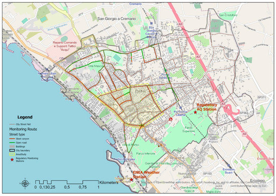
Figure 1.
Map of the City of Portici. The map includes: the weather station (by ENEA RC Portici) and the regulatory air quality monitoring station located in the city (both represented in red stars); the area study (represented in the yellow area) and the urban street network classified as street canyon (red lines) and open street (green lines).
Air quality in the city of Portici is monitored by a single monitoring station maintained by the Regional Agency of Environmental Protection (ARPAC). This is a background monitoring station, located within a park (Figure 1), at about 80 m on the sea level. The height of the sampling point is at about 3.5 m from the ground. The measurement equipment and operating methods meet the standards established by the European Community (2008/50/CE). From the meteorological point of view, the city is characterized by a breeze regime, as almost all coastal towns are. Prevailing winds are mainly from S to SW during spring and summer, and mainly from N to NE during autumn and winter. The most frequent classes of wind velocity are the 1–2 m/s [7].
For our research, a pivotal neighborhood of the city has been considered, crossed by the road network of the city center. The network consists of four main urban roads—Via Libertà, Via Da Vinci, Via Diaz, and Corso Garibaldi (Figure 2). The latter, along with Via Libertà, are the roads which sustain most of inbound/outbound traffic from/to the city area.
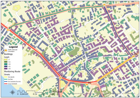
Figure 2.
Map of the selected neighborhood of the City of Portici including footprint of the buildings with their height, the monitoring route—Via Libertà (yellow line), Via da Vinci (blue line), Via Diaz (green line), Corso Garibaldi (red line) —and the locations of the traffic vehicular campaigns.
The urban canopy layer (the layer of air extending from the ground surface up to the level of the buildings) of the selected neighborhood is composed of numerous street canyons, which are narrow urban roads, flanked by a continuous row of high buildings on both sides. These street canyons promote the accumulation of traffic-induced pollution, due to their lack of natural ventilation, so that, along these roads, the human exposure to air pollution is higher. It is also known that the street levels of pollution can vary widely between canyons, due to the meteorological conditions, to the difference in emissions, and to the variation in the street canyon morphology (e.g., the ratio between building height [H] and width [W]).
Identifying the street canyon effects across an urban area can help to understand the spatial variability of pollutant concentrations that can be captured by using air dispersion models at district scale as SIRANE as well as a pervasive monitoring [7].
For our scope, using the 3D urban model of the City of Portici, including buildings and vegetation, performed by the authors in a previous research work [7], the geometric attributes (i.e., width and length) of the selected urban roads and the buildings’ height along these roads have been derived and the spatial layer of street canyons has been generated. This layer (Figure 1) classifies every selected urban road as a street canyon if the ratio W/H ≤ 3 and, otherwise, is an open road. Figure 1 shows that the four roads selected are street canyons for almost their entire length. It has to be noted that in a street canyon, the pollutant concentrations increase near the ground due to the phenomena of recirculation that lead to pollutants stagnation. Thus, the spatial variability in (local) concentrations can be captured by the mobile device MONICA, used in this research. MONICA can be easily carried in the hand or in a backpack of any citizen, eventually involved in (opportunistic) mobile monitoring campaigns, during walk along the city streets [22,23].
2.2. Mobile Monitoring Campaigns
MONICA (Cooperative Air Quality Monitoring multi-sensor platform) [21], has been set up with fixed time slots and a fixed route of about 2.5 km, including the streets of Via Libertà, Via Da Vinci, Via Diaz, and Corso Garibaldi (Figure 2), during two working days in June (5, 21 June 2019). Considering that school activity, in an urban area, significantly contributes to the urban vehicular traffic during the morning rush hours, two working days in June have been selected. The first one was selected when the schools were still open, and the second one was selected during the summer holidays, i.e., when the vehicular traffic was essentially caused by the human activities other than those related to schools (e.g., working, leisure, sportive, in-home maintenance activities).
The sensing platform MONICA used for mobile monitoring is a low-cost air quality monitoring portable multisensory device. With a volume footprint of (15 × 15 × 5 cm3), it hosts an array of solid-state sensors which include three Electrochemical sensors (Alphasense B4 class CO, NO2, O3 targeted sensors) along with their analog front end. Sensor data are gathered through a uC based board (Nucleo LK432KC) whose firmware is responsible for continuous acquisition of raw data and its transmission through BLE interface. Usually interfaced with the user smartphone, MONICA platform exploits an Android APP calibrating raw data and extracting concentration estimations through AI (Artificial Intelligence) components, previously trained with field calibration campaigns [21]. The APP also provides immediate feedback to the user bearing the device. This Android app has been developed and designed to provide local and immediate feedback to the user, exploiting the above-mentioned, on-board AI driven calibration components. Estimated concentrations for the target gases are numerically reported to the concerned user along with a colorimetric index for holistic air quality assessment. The latter is based on European AQI structure (EAQI), and compares the estimated concentrations with threshold values derived from the current regulative framework, i.e., the 2008 European Air Quality Directive. Concentrations of single target gases are also reported using a similar color scale which highlight their influence on the holistic index. In this way, the user can obtain immediate feedback in terms of recommendations linked to the EAQI while being capable to identify at a glance which pollutant is responsible for Air Quality degradation in case of harsh conditions.
One of the main concerns when using low-cost, solid-state, sensor-based Air Quality Multisensor systems is the quality and accuracy of the data. In terms of data coverage, due to the reliability of the BT connectivity and the smartphone centered solution, the MONICA devices have shown their capability to exceed 99% data delivery. In terms of accuracy, since MONICA nodes are based on electrochemical devices, they are subject to environmental influences and to cross interference by non-target gases which elicit an unwanted response on their electrodes. In particular, the employed Alphasense NO2 sensor is subject to limited but significant influence of high O3 concentrations. To reduce the impact of these interferences, nodes were calibrated using state of the art methodology, ensuring the best available accuracy for this class of sensors which is field-calibrated by colocation with regulatory grade analyzers. The calibration law is a multilinear regression including both NO2 and O3 sensors’ raw responses (Working and Auxiliary electrodes voltage) as regressors along with temperature readings, so to correct for their influence on multisensory device concentration estimations. The colocation period has been performed in similar environmental conditions in the same city so to provide for minimum performance degradation due to concept drift effects [21]. With this information, the best accuracy setup for the proposed experiments can be ensured. Short-term accuracy figures of the devices are highlighted in [21].
The gathered estimations along with raw data are transmitted to a backend/frontend IoT device management platform which takes care of storage and data presentation tasks. Battery operated (3.7 V 3800 mA), it can sustain more than 20 h of continuous monitoring before a recharge is needed, being thus compatible with the smartphone companion use case. A recent version has been equipped with an Optical Particle Counter (Plantower PMS7003) for PM sensing duties [22,23].
The monitoring campaign has consisted of 6 runs (Figure 3), repeated at two different days and different times on one day. During a run, two passages have been made by each location taking 1 h. A passage denotes the completion of the entire route once. The entire monitoring campaign has collected 6 h of point measurements along the selected route. This sampling schema has been designed to make comparable concentration measurements with concentration estimations by the SIRANE model. In fact, this latter estimates hourly average values of the air pollution concentrations along street segments properly characterized according to their geometry and that of the surrounding buildings.
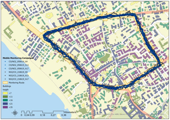
Figure 3.
Maps of the mobile monitoring campaigns along the selected monitoring route.
Each run started at the city square of San Ciro (SQ in Figure 2) continued along Via Libertà, turning to Via da Vinci and then to Corso Garibaldi until reaching the city square. The runs have covered the rush hours in the morning (from 9 a.m. to 10 a.m.), at the lunchtime (from 1 p.m. to 2 p.m.), and in the evening (from 5 p.m. to 6 p.m.). The concentrations of CO and NO2 have been measured walking along the route at 1/6 Hz time resolution and at about 1m in height from the street level.
The monitoring campaigns have been designed to guarantee an appropriate temporal and spatial coverage and to address the research questions.
2.3. Traffic Vehicular Campaigns
During mobile monitoring campaigns, vehicular traffic has been monitored in five strategic locations: in San Ciro Square (SQ) and at the four road junctions along the monitoring route. These latter are the road junction of via Garibaldi and via Gianturco (C1), the road junction of Via Diaz and Via Garibaldi (C2), the road junction of Via Diaz and Via da Vinci (C3), and the road junction of Via Libertà and Via Da Vinci (C4) (Figure 2).
By using hand-held cameras, the number of vehicles travelling for the crossroads has been monitored during the first and the last 10 min of each rush hour in the two days of mobile monitoring campaigns. Processing point data collected on one hour, the average number of vehicles per hour, along each street segment of the route, have been derived. In particular, the number of vehicles along each street segment has been calculated by the difference among the numbers of the vehicles at monitoring points, while the average number of vehicles per minute has been calculated by dividing the number of vehicles monitored in one rush hour for the length of the entire monitoring period. Additionally, the vehicles monitored have been classified into 5 categories: cars, motorcycles, light duty vehicles and heavy-duty vehicles, and buses, according to the COPERT classification [24].
2.4. SIRANE Air Pollution Maps
The scope of this work has been to investigate the ability of a dispersion model such as SIRANE to capture the local variability of pollutant concentrations at the urban scale by comparing the estimated concentrations with mobile measurements. To do this, maps of air pollutants’ concentrations at high spatial resolution have been performed by using the model SIRANE (Figure A1, Figure A2, Figure A3, Figure A4, Figure A5 and Figure A6).
SIRANE is an operational model at the local urban scale. It simulates pollutant dispersion within and above the urban canopy scale and provides hourly averaged pollutant concentrations within each street, assuming steady meteorological conditions over hourly time steps [14]. SIRANE is based on a street network approach and represents the urban canopy as a network of connected streets whose relative pollutant exchange is modeled adopting ad hoc parameterizations, notably considering three exchange processes [25] as the advection of pollutant along the street axis [26], the dispersion at the intersections [27], and the ventilation through the turbulent exchange at the roof level [28]. Above the canopy, SIRANE is integrated with a Gaussian plume model. Further details on the model are provided in [14]. Over the last two decades, SIRANE has been widely used [29,30,31,32,33,34,35,36] and has been validated both in wind tunnel [37,38] and in field trough fixed air quality monitoring stations.
For our scope, six maps for both the pollutant NO2 and CO have been performed using SIRANE in order to compare the estimations by the model with measurements by MONICA.
For running SIRANE, several input datasets have been collected and/or processed as the urban geometry including the street network and buildings, the meteorological data, the linear emissions, and the background concentrations.
In particular, for calculating the traffic emissions, firstly an average emission factor for each category of vehicles and for both CO and NO2 has been estimated. To this data of the metropolitan vehicular fleet database, published by the Automobile Club d’Italia (ACI) have been used together with the emission factors computed by the Istituto Superiore per la Protezione e la Ricerca Ambientale (ISPRA) by means of the COPERT model [24]. Then, the emissions have been estimated by multiplying the emission factors by the number of vehicles monitored during the vehicular traffic campaigns, as above described.
Background concentration of all pollutants was given to SIRANE as hourly averaged concentration homogeneous in all the area study and equal to hourly averaged concentration measured by the regulatory monitoring station, located at the City of Portici (Figure 1). They have been processed by SIRANE before applying the chemistry module within SIRANE.
The meteorological data taken in input by SIRANE is collected by the ENEA meteorological station (Figure 1).
The monitoring route, taken in input by SIRANE, is subdivided into homogeneous segments, having the same geometry (i.e., the same width and aspect ratio). Along this route, a number of 62 homogenous segments have been identified, and 47 have been identified as street canyons. The geometric characteristics of the street segment of the monitoring route have been derived from the 3D city model, previously performed. In Table 1, an overview of these characteristics is reported.

Table 1.
Overview of the characteristics of the monitoring route.
The SIRANE model evaluates the averaged value of the concentrations of the pollutants over the whole volume of each street segment properly identified. SIRANE returns the output as hourly maps of the pollutant concentrations at street scale as well as point estimation (named receptor point) of the pollutant concentrations associated with each identified street segment (Figure 4).
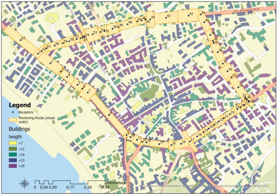
Figure 4.
Map of the receptor points and the polygon street segments at which SIRANE associates the estimated pollutant concentrations.
3. Results and Discussion
The capability of the SIRANE model of capturing the local spatial variability of pollutant concentrations along the urban roads has been investigated in this work by comparing the estimated concentrations of NO2 and CO pollutants with the mobile measurements of these pollutants gathered by the MONICA ecosystem.
The assumption of background concentration spatially homogeneous on the area of interest and equal to hourly average values measured at a reference background station follows the guidelines of developers in the use of SIRANE.
Firstly, the traffic vehicular data, collected during the two campaigns, has been analyzed in order to characterize the main source of the air pollution by NO2 and CO in the City of Portici.
In Table 2, it can be seen that the traffic volume of first campaign (5 June) is greater than that in the second campaign (21 June), in all rush hours and mostly in the morning. In this regard, we can observe that, in the first monitoring day, the morning hours included the entry and exit time from schools while in the second monitoring day the schools were closed, thus explaining the difference in the traffic volume monitored.
Table 2.
Overview of traffic vehicular campaigns.
Analyzing the single campaign, on 5 June, the greatest traffic volume has been recorded in the evening hour (17:00–18:00) with 105,539 vehicles, while on 21 June, the greatest number of vehicles has been recorded in the lunchtime hour (13:00–14:00) with 88,610 vehicles.
However, the busiest street has been Corso Garibaldi with an average traffic of 36,255 on the first monitoring day and of 32,386 on the second monitoring day. Although, the recorded traffic volume has shown little change over the two monitoring days. The reason could be that it is one of the inbound/outbound streets to/from the city. Finally, the street with less traffic is Via Da Vinci with an average number of vehicles of 11,125 on the monitoring day first and of 7461 on the second one.
Grouping by different vehicle category, a characterization of the vehicle fleet for both monitoring days is shown in the graphs reported in Figure 5.
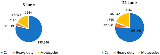
Figure 5.
The vehicle feet by the two traffic monitoring campaigns grouped by vehicle category.
The car category is the largest, including 79% and 76% of vehicles monitored in the first and second traffic campaign, respectively. The motorcycles category counts for about 16% of vehicles by the first monitoring day and 18% by the second monitoring day. The other vehicle categories, instead, include the same number of vehicles in the two monitoring days and are, respectively, 5% for heavy duty vehicles, 1% for light duty vehicles, and 1% for bus.
The insight on the vehicle feet has been here performed for the calculation of the traffic emissions that SIRANE model takes in input. Significant sources, different from vehicular traffic, are not present in the area. Therefore, their emissions were not considered.
As regards concentrations, the data analysis has been performed by spatially aggregating the measured and estimated data at two different spatial scales. The selected spatial entities have been the entire monitoring route and the segments of varying length within the route, classified as street canyons and open roads. The mobile and estimated data have been spatially aggregated by allocating them to the spatial entities on the basis of their spatial coordinates (i.e., GPS data). Additionally, working at segment scale, they have been associated with the central points of the segments, named receptor points. Thus, the mobile data allocated has been aggregated by calculating the arithmetic mean while the estimated data has been performed as average value over the whole volume of the segment. The data aggregations have been performed for every monitored hush hour.
Aggregating the concentration data on the entire monitoring route and for each monitored rush hour, it has been observed that the measured concentrations of both CO and NO2 have an overall average value higher than the estimated average concentrations. In particular, this difference is higher by a factor of 3 for CO concentrations, while for NO2 concentrations the factor is 2. The graphs of Figure 6 show these results for each monitored hush hour. The error bars are calculated as the standard deviation of the time-averaged concentrations for each segment.
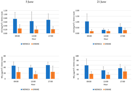
Figure 6.
Comparison between the average measured and estimated concentrations of CO and NO2 pollutants, by aggregating data spatially distributed along the entire monitoring route and for each monitored hush hour.
Additionally, according to the segment classification of the monitoring route, the collected data has been aggregated by calculating the overall average of point data allocated to the street canyon segments and open street segments, respectively.
In relation to street canyon segments, we have observed that the difference factors between the mean recorded and simulated concentrations increase for both CO and NO2 compared to the factors observed for the entire route, exactly from 3 to 3.3 for CO and from 2 to 2.3 for NO2. On the contrary, in relation to open street segments, the difference factors decrease compared to the related factors calculated along the entire route, exactly from 3 to 2.5 for CO, and from 2 to 1.9 for NO2. The graphs of Figure 7 and Figure 8 show these differences for each monitored rush hour.
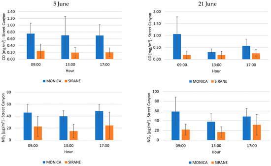
Figure 7.
Comparison between the average measured and estimated concentrations of CO and NO2 pollutants in relation to the street canyon segments.
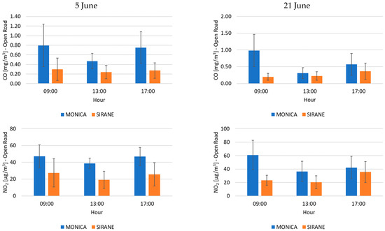
Figure 8.
Comparison between the average measured and estimated concentrations of CO and NO2 pollutants in relation to the open street segments.
The next step has been to analyze the variability of NO2 and CO concentrations at segment scale. At this scope, the mean concentrations profiles of NO2 and CO pollutants have been generated by aggregating the mobile data on the identified segments and calculating the overall average of the allocated data as well as deriving the average estimation associated with the receptor points. The graphs of Figure 9 and Figure 10 show these profiles for the 62 street segments identified along the monitoring route and classified as street canyons and open streets.
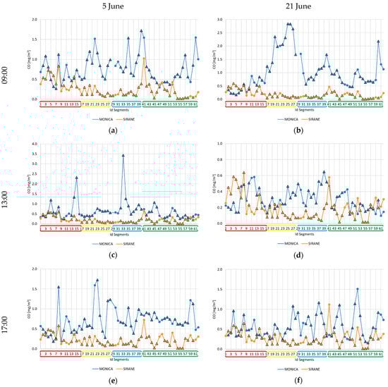
Figure 9.
Comparison between MONICA (blue line) and SIRANE (orange line), for CO pollutant: (a) at 9 am on 5 June; (b) at 9 am on 21 June; (c) at 1 am on 5 June; (d) at 1 am on 21 June; (e) at 5 pm on 5 June; (f) at 5 pm on 21 June. Triangles are street canyons and circle open roads. The ID receptors from 1 to 16 (red lines) are referred to the road segment Corso Garibaildi; IDs from 17 to 28 (yellow lines) to the road segment Via Libertà; IDs from 29 to 40 (blue lines) to the road segment Via DaVinci; IDs from 41 to 61 (green lines) to the road segment Via Diaz.
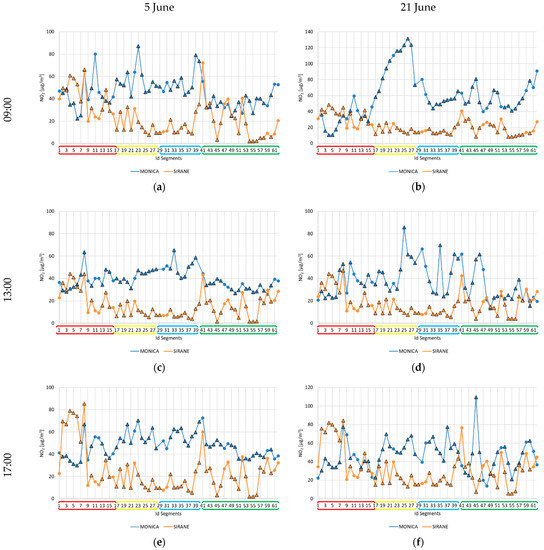
Figure 10.
Comparison between MONICA (blue line) and SIRANE (orange line), for NO2 pollutant: (a) at 9 am on 5 June; (b) at 9 am on 21 June; (c) at 1 am on 5 June; (d) at 1 am on 21 June; (e) at 5 pm on 5 June; (f) at 5 pm on 21 June. Triangles are street canyons and circle open roads. The ID receptors from 1 to 16 (red lines) are referred to the road segment Corso Garibaildi; IDs from 17 to 28 (yellow lines) to the road segment Via Libertà; IDs from 29 to 40 (blue lines) to the road segment Via DaVinci; IDs from 41 to 61 (green lines) to the road segment Via Diaz.
Broadly, the patterns in these concentration profiles correspond. The concentration profiles exhibit the same peaks, following roughly the same spatial trend. However, the simulated concentration profiles appear smoother than the measured concentration ones. In this regard, it is to be noted that, in the mobile profiles, sharp peaks are observed probably due to events that occurred during the monitoring run and causing local high pollutant concentrations, such as a closely passing car or bus, or walking in the emission plume right behind a vehicle, or even idling vehicles due to local traffic congestion.
It is known that these events can occur systematically at certain places or can be more accidental. If they are systematic, they are usually modeled by SIRANE as well as captured by MONICA. Otherwise, if they randomly occur, they might not be modeled by SIRANE, especially if they are sharp peaks, while they are captured by MONICA. Just as an example, looking at the peak at segment ID 33 in the CO profile of Figure 9c, it is evident that this peak is captured in its high magnitude by MONICA while smoothed by SIRANE. Most probably, that is one of those accidental events above specified.
The differences observed between measured and estimated pollutant concentrations may be attributed to several factors. A first factor is given from the operation conditions of MONICA during the mobile monitoring campaigns. MONICA, as mobile device, has been carried in hand during the campaigns, gathering measurements at about 1 m from street level, on one side of the street and on the sidewalk. Thus, these operation conditions have allowed measurements of higher pollutant concentrations to be gathered.
On the other hand, SIRANE evaluates the average concentration of a pollutant within the whole volume of the homogeneous segment. In fact, in the literature, when SIRANE is compared with air quality monitoring stations [39] or passive samplers [40] located 3–4 m above the streets, the simulated trends, except for the unavoidable under-estimation of some peaks of pollution, fit very well in the measurements, with a good correlation.
Another factor that can justify the observed results is the estimation of the emissions. In the SIRANE model, the emission data is evaluated by using an average emission factor weighted by vehicle type on the vehicle fleet registered in one year. Thus, SIRANE does not take into account the presence of any high emitters as high-emission vehicles (HEVs), which could cause concentration peaks [41], as those captured by MONICA during the mobile monitoring campaigns did.
4. Conclusions
Capturing the local variability in air pollutant concentrations across an urban area is a key issue to assess the urban air quality at high spatial resolution and to evaluate the population exposure to high pollutant concentration levels. To date, the approaches available are essentially based on a pervasive air quality monitoring using fixed and mobile sensor networks and on air dispersion modeling at fine length scales. Their potential has been investigated in literature showing both the uncertainty in the average concentration levels and the limits in identifying air pollution hot spots within the city.
In this study, we have investigated the capability of an operational air dispersion model at district scale, such as SIRANE, in identifying the local spatio-temporal variability of pollutant concentrations within an urban district, with respect to mobile monitoring campaigns, using low-cost sensor devices. By comparing the mean concentrations of CO and NO2 pollutants measured by MONICA devices and those simulated by SIRANE along the urban streets, we have shown that the recorded concentrations appear exceeding the simulated ones by a factor of 3 and 2 for CO and for NO2, respectively. Furthermore, for both the pollutants, this factor is higher within the street canyons than in open roads.
However, the data recorded and the simulated pollutant concentrations show patterns that broadly correspond, and also the peaks observed in the mobile profiles appear in the simulated profiles, though smoothed. All of this has been explained by (i) the different height of the receptor points at street level; MONICA measures pollutants concentrations at about 1 m height while SIRANE evaluates the spatially averaged concentration in each street segment; (ii) the uncertainty in the estimation of vehicle emissions in SIRANE that does not take into account the presence of high-emitting vehicles; and (iii) the different temporal resolution of measurements gathered by MONICA capable to capture local high concentrations. Thus, a further potential research could include (i) the use of MONICA devices at different heights for a better understanding of the differences between measured and modeled concentrations, and (ii) the participation of the citizens for more pervasive monitoring campaigns.
However, the results demonstrate that an air dispersion model at district scale as SIRANE can indeed be used for a first evaluation of the urban air pollution. An integrated approach, including a pervasive air quality monitoring by mobile or opportunistic campaigns, may be necessary for applications related to hotspot identification, personal exposure studies, and/or high-resolution mapping. Mobile as well as opportunistic monitoring campaigns will have to collect sufficient data to cover both spatial and temporal variability. Such integrated approach can be feasible if low-cost air quality sensors are available that can collect reliable data in an effortless way.
Author Contributions
Conceptualization, G.F., A.C., F.M. and D.T.; Methodology, G.F., A.C., D.T. and F.M.; Modeling, Data analysis and geospatial analysis, G.F., A.C. and D.T.; Validation, F.M., S.D.V. and M.F.; Monitoring campaigns, D.T., A.C., G.F., F.M. and M.F.; Investigation, F.M., D.T. and G.F.; data curation and node calibration, G.F., D.T. and S.D.V.; writing—original draft preparation, curation, G.F. and D.T.; writing—review and editing, G.F., D.T., S.D.V., F.M., M.F. and G.D.F.; visualization, G.F. and D.T.; supervision, F.M., M.F. and G.D.F. All authors have read and agreed to the published version of the manuscript.
Funding
This research received no external funding.
Data Availability Statement
The data presented in this study are available on request from the corresponding author.
Acknowledgments
The authors acknowledge Giampiero Sorrentino for his involvement in the monitoring campaigns, Pietro Salizzoni and the research group of AIR—Atmosphere, Impact & Risk from Ecole Centrale de Lyon (France) for providing us the SIRANE model and the research group of the Photovoltaic and Sensor Applications Laboratory (Lab. SAFS) at ENEA RC Portici (Italy) for providing the devices MONICA and recorded data properly calibrated.
Conflicts of Interest
The authors declare no conflict of interest.
Appendix A
The map of simulated CO and NO2 concentrations generated by SIRANE are shown in Figure A1, Figure A2, Figure A3, Figure A4, Figure A5 and Figure A6.

Figure A1.
Maps of the estimated concentrations on 5 June at 9 a.m.: (a) CO concentrations; (b) NO2 concentrations.

Figure A2.
Maps of the estimated concentrations on 5 June at 1 a.m.: (a) CO concentrations; (b) NO2 concentrations.

Figure A3.
Maps of the estimated concentrations on 5 June at 5 p.m.: (a) CO concentrations; (b) NO2 concentrations.

Figure A4.
Maps of the estimated concentrations on 21 June at 9 a.m.: (a) CO concentrations; (b) NO2 concentrations.

Figure A5.
Maps of the estimated concentrations on 21 June at 1 a.m.: (a) CO concentrations; (b) NO2 concentrations.

Figure A6.
Maps of the estimated concentrations on 21 June at 5 p.m.: (a) CO concentrations; (b) NO2 concentrations.
References
- European Environment Agency. Europe’s Air Quality Status 2020 Report. Available online: https://www.eea.europa.eu/publications/status-of-air-quality-in-Europe-2022 (accessed on 31 October 2022).
- Toscano, D.; Murena, F. The historical trend of air pollution and its impact on human health in Campania region (Italy). Atmosphere 2021, 12, 553. [Google Scholar] [CrossRef]
- Vardoulakis, S.; Solazzo, E.; Lumbreras, J. Intra-urban and street scale variability of BTEX, NO2 and O3 in Birmingham, UK: Implications for exposure assessment. Atmos. Environ. 2011, 45, 5069–5078. [Google Scholar] [CrossRef]
- Peters, J.; Van den Bossche, J.; Reggente, M.; Van Poppel, M.; De Baets, B.; Theunis, J. Cyclist exposure to UFP and BC on urban routes in Antwerp, Belgium. Atmos. Environ. 2014, 92, 31–43. [Google Scholar] [CrossRef]
- Murena, F.; Prati, M.V. Spatial variability of fine particle number concentration in an urban area. In Proceedings of the Seventh International Conference on Environmental Management, Engineering, Planning and Economics (CEMEPE 2019) and SECOTOX Conference, Mykonos Island, Greece, 19–24 May 2019; pp. 19–24. [Google Scholar]
- Wilson, J.G.; Kingham, S.; Pearce, J.; Sturman, A.P. A review of intraurban variations in particulate air pollution: Implications for epidemiological research. Atmos. Environ. 2005, 39, 6444–6462. [Google Scholar] [CrossRef]
- Fattoruso, G.; Nocerino, M.; Toscano, D.; Pariota, L.; Sorretino, G.; Manna, V.; De Vito, S.; Carteni, A.; Fabbricino, M.; Di Francia, G. Site suitability analysis for low-cost sensor networks for urban spatially dense air pollution monitoring. Atmosphere 2020, 11, 1215. [Google Scholar] [CrossRef]
- Apte, J.S.; Messier, K.P.; Gani, S.; Brauer, M.; Kirchstetter, T.W.; Lunden, M.M.; Marshall, J.D.; Portier, C.J.; Vermeleu, R.C.H.; Hamburg, S.P. High-resolution air pollution mapping with Google street view cars: Exploiting big data. Environ. Sci. Technol. 2017, 51, 6999–7008. [Google Scholar] [CrossRef] [PubMed]
- Steffens, J.; Kimbrough, S.; Baldauf, R.; Isakov, V.; Brown, R.; Powell, A.; Deshmukh, P. Near-port air quality assessment utilizing a mobile measurement approach. Atmos Pollut Res. 2017, 8, 1023–1030. [Google Scholar] [CrossRef]
- Ye, Q.; Gu, P.; Li, H.Z.; Robinson, E.S.; Lipsky, E.; Kaltsonoudis, C.; Lee, A.K.Y.; Apte, J.S.; Robinson, A.L.; Sullivan, R.C.; et al. Spatial variability of sources and mixing state of atmospheric particles in a metropolitan area. Environ. Sci. Technol. 2018, 52, 6807–6815. [Google Scholar] [CrossRef]
- Esposito, E.; De Vito, S.; Salvato, M.; Fattoruso, G.; Di Francia, G. Computational intelligence for smart air quality monitors calibration. In Computational Science and Its Applications; LNCS; Springer: Cham, Switzerland, 2017; Volume 10406, pp. 443–454. [Google Scholar]
- Zwack, L.M.; Hanna, S.R.; Spengler, J.D.; Levy, J.I. Using advanced dispersion models and mobile monitoring to characterize spatial patterns of ultrafine particles in an urban area. Atmos. Environ. 2011, 45, 4822–4829. [Google Scholar] [CrossRef]
- Merbitz, H.; Fritz, S.; Schneider, C. Mobile measurements and regression modeling of the spatial particulate matter variability in an urban area. Sci. Total Environ. 2012, 438, 389–403. [Google Scholar] [CrossRef]
- Soulhac, L.; Salizzoni, P.; Cierco, F.X.; Perkins, R. The model SIRANE for atmospheric urban pollutant dispersion; PART I, presentation of the model. Atmos. Environ. 2011, 45, 7379–7395. [Google Scholar] [CrossRef]
- CERC. ADMS-Urban. 2016. Available online: http://www.cerc.co.uk/ADMS-Urban (accessed on 31 October 2022).
- Wallace, J.; Corr, D.; Deluca, P.; Kanaroglou, P.; McCarry, B. Mobile monitoring of air pollution in cities: The case of Hamilton, Ontario, Canada. J Environ Monitor. 2009, 11, 998–1003. [Google Scholar] [CrossRef] [PubMed]
- Zwack, L.M.; Paciorek, C.J.; Spengler, J.D.; Levy, J.I. Characterizing local traffic contributions to particulate air pollution in street canyons using mobile monitoring techniques. Atmos. Environ. 2011, 45, 2507–2514. [Google Scholar] [CrossRef]
- Van den Bossche, J.; Peters, J.; Verwaeren, J.; Botteldooren, D.; Theunis, J.; De Baets, B. Mobile monitoring for mapping spatial variation in urban air quality: Development and validation of a methodology based on an extensive dataset. Atmos. Environ. 2015, 105, 148–161. [Google Scholar] [CrossRef]
- Hasenfratz, D.; Saukh, O.; Walser, C.; Hueglin, C.; Fierz, M.; Arn, T.; Beutel, J.; Thiele, L. Deriving high-resolution urban air pollution maps using mobile sensor nodes. Pervasive Mob Comput. 2015, 16, 268–285. [Google Scholar] [CrossRef]
- Van den Bossche, J.; Theunis, J.; Elen, B.; Peters, J.; Botteldooren, D.; De Baets, B. Opportunistic mobile air pollution monitoring: A case study with city wardens in Antwerp. Atmos. Environ. 2016, 141, 408–421. [Google Scholar] [CrossRef]
- De Vito, S.; Esposito, E.; Massera, E.; Formisano, F.; Fattoruso, G.; Ferlito, S.; Del Giudice, A.; D’Elia, G.; Salvato, M.; Polichetti, T.; et al. Crowdsensing IoT architecture for pervasive air quality and exposome monitoring: Design, development, calibration, and long-term validation. Sensors 2021, 21, 5219. [Google Scholar] [CrossRef]
- De Vito, S.; Fattoruso, G.; D’Elia, G.; Esposito, E.; Ferlito, S.; Del Giudice, A.; Massera, E.; Loffredo, G.; Di Francia, G. Hyper resoluted air quality maps in urban environment with crowdsensed data from intelligent low cost sensors. In Proceedings of the 2022 IEEE International Symposium on Olfaction and Electronic Nose (ISOEN), 29 May–1 June 2022; pp. 1–4. [Google Scholar]
- Peruzzi, C.; Ramel-Delobel, M.; Coudon, T.; Fervers, B.; De Vito, S.; Fattoruso, G.; Salizzoni, P. Air pollution measurements during commuting in Lyon (No. EGU22-13150). In Proceedings of the EGU General Assembly 2022, Vienna, Austria, 23–27 May 2022. [Google Scholar]
- Ntziachristos, L.; Gkatzoflias, D.; Kouridis, C.; Samaras, Z. COPERT: A European road transport emission inventory model. In Information Technologies in Environmental Engineering; Springer: Berlin/Heidelberg, Germany, 2009; pp. 491–504. [Google Scholar]
- Soulhac, L.; Salizzoni, P.; Mejean, P.; Perkins, R.J. Parametric laws to model urban pollutant dispersion with a street network approach. Atmos. Environ. 2013, 67, 229–241. [Google Scholar] [CrossRef]
- Soulhac, L.; Perkins, R.J.; Salizzoni, P. Flow in a street canyon for any external wind direction. Boundary-Layer Meteorol. 2008, 126, 365–388. [Google Scholar] [CrossRef]
- Soulhac, L.; Garbero, V.; Salizzoni, P.; Mejean, P.; Perkins, R.J. Flow and dispersion in street intersections. Atmos. Environ. 2009, 43, 2981–2996. [Google Scholar] [CrossRef]
- Salizzoni, P.; Soulhac, L.; Mejean, P. Street canyon ventilation and atmospheric turbulence. Atmos. Environ. 2009, 43, 5056–5067. [Google Scholar] [CrossRef]
- Soulhac, L.; Salizzoni, P.; Mejean, P.; Didier, D.; Rios, I. The model SIRANE for atmospheric urban pollutant dispersion; PART II, validation of the model on a real case study. Atmos. Environ. 2012, 49, 320–337. [Google Scholar] [CrossRef]
- Soulhac, L.; Nguyen, C.V.; Volta, P.; Salizzoni, P. The model SIRANE for atmospheric urban pollutant dispersion. PART III: Validation against NO2 yearly concentration measurements in a large urban agglomeration. Atmos. Environ. 2017, 167, 377–388. [Google Scholar] [CrossRef]
- Biemmi, S.; Gaveglio, R.; Salizzoni, P.; Boffadossi, M.; Casadei, S.; Bedogni, M.; Carbero, V.; Soulhac, L. Estimate of boundary layer parameters and background concentrations for pollutant dispersion modeling in urban areas. In Proceedings of the 31st NATO/SPS International Technical Meeting on Air Pollution Modelling and its Application, Torino, Italy, 27 September–1 October 2010; p. 27. [Google Scholar]
- Castagnetti, F.B.; Salizzoni, P.; Garbero, V.; Genon, G.; Soulhac, L. Atmospheric pollution modelling in urban areas at local scale: An example of the application to a neighborhood in Turin. Geoing Ambient E Min. 2008, 124, 63–76. [Google Scholar]
- Garbero, V.; Salizzoni, P.; Soulhac, L. Experimental study of pollutant dispersion within a network of streets. Boundary-Layer Meteorol. 2010, 136, 457–487. [Google Scholar] [CrossRef]
- Giambini, P.; Salizzoni, P.; Soulhac, L.; Corti, A. Air quality modelling system for traffic scenario analysis in Florence: Model validation and identification of critical issues. In Proceedings of the 13th International Conference on Harmonisation within Atmospheric Dispersion Modelling for Regulatory Purposes (HARMO 2010), Paris, France, 1–4 June 2010; pp. 195–199. [Google Scholar]
- Pognant, F.; Bo, M.; Nguyen, C.V.; Salizzoni, P.; Clerico, M. Modelling and evaluation of emission scenarios deriving from wood biomass boilers in alpine valley. In Proceedings of the 18th International Conference on Harmonisation within Atmospheric Dispersion Modelling for Regulatory Purposes (HARMO 2017), Bologna, Italy, 9–12 October 2017; pp. 9–12. [Google Scholar]
- Pognant, F.; Bo, M.; Nguyen, C.V.; Salizzoni, P.; Clerico, M. Design, modelling and assessment of emission scenarios resulting from a network of wood biomass boilers. Environ. Model. Assess. 2018, 23, 157–164. [Google Scholar] [CrossRef]
- Salem, N.B.; Garbero, V.; Salizzoni, P.; Lamaison, G.; Soulhac, L. Modelling pollutant dispersion in a street network. Boundary-Layer Meteorol. 2015, 155, 157–187. [Google Scholar] [CrossRef]
- Carpentieri, M.; Salizzoni, P.; Robins, A.; Soulhac, L. Evaluation of a neighbourhood scale, street network dispersion model through comparison with wind tunnel data. Environ. Model. Softw. 2012, 37, 110–124. [Google Scholar] [CrossRef]
- Bo, M.; Charvolin-Volta, P.; Clerico, M.; Nguyen, C.V.; Pognant, F.; Soulhac, L.; Salizzoni, P. Urban air quality and meteorology on opposite sides of the Alps: The Lyon and Torino case studies. Urban Clim. 2020, 34, 100698. [Google Scholar] [CrossRef]
- Bo, M.; Salizzoni, P.; Pognant, F.; Mezzalama, R.; Clerico, M. A combined citizen science—Modelling approach for NO2 assessment in Torino urban agglomeration. Atmosphere 2020, 11, 721. [Google Scholar] [CrossRef]
- Murena, F.; Toscano, D. High emitting vehicles and sustainable development of urban areas. In Proceedings of the 13th International Conference on Air Quality—Science and Application, Thessalonik, Greece, 27 June–1 July 2022. [Google Scholar]
Publisher’s Note: MDPI stays neutral with regard to jurisdictional claims in published maps and institutional affiliations. |
© 2022 by the authors. Licensee MDPI, Basel, Switzerland. This article is an open access article distributed under the terms and conditions of the Creative Commons Attribution (CC BY) license (https://creativecommons.org/licenses/by/4.0/).