Abstract
Through chaos theory, experimental data of hourly time series are analyzed. These time series consist of Radon concentration levels and meteorological variables of temperature, pressure, and relative humidity within the boundary layer and very close to the ground. Results were obtained in two urban dwellings for family use and for two different periods of time, of the order of one month and one month plus one week, respectively. Each time series was subjected to a chaotic analysis showing the existence of the characteristic chaotic parameters in the appropriate ranges: Lyapunov coefficient (λ), correlation dimension (Dc), Kolmogorov entropy (SK), Lempel-Ziv complexity (LZ), Hurst coefficient (H), maximum predictability time (τ), lost information (<ΔI>) and fractal dimension (D). The studied processes show to be irreversible. From the chaotic parameters, it is shown that the ratio between the entropy of each meteorological variable and the radon concentration is very sensitive to relative humidity. Likewise, the meteorological variables that most affect the concentration of Radon are relative humidity and temperature. The concordance between the results obtained and those delivered by analyzes carried out through other methodologies in longer periods is verified.
1. Introduction
Micrometeorology is a line of study for meteorology to related observations and processes on smaller scales of space and time [1,2], of the order of 1 km and measurement periods of one day or smaller. These processes are limited to the lower part of the planetary boundary layer, known as the atmospheric boundary layer (ABL). Multiple internal boundary layers are characterized by high connectivity, mixtures, and turbulent movements, influenced by friction with the Earth’s surface [2,3]. In this stratified atmospheric region, there is an exchange of energy, mass, and gases with the irregular surface of the earth composed of water, soil, vegetation, and the results of human activity. The surface of the earth and its heterogeneous components represent a limit that greatly influences the atmosphere, mainly the properties of the air in the ABL. The effects of friction, the rise, and fall of the surface temperature stimulate a great movement of the air, a flow that makes possible the transport of momentum, heat, humidity, or matter [3]. Temperature and wind (turbulence) are affected by external factors, such as buildings [4], flora, population, and relief, which makes their study relevant. Currently, there are international networks that provide information on flows. These networks indicate which application of micrometeorological techniques is most suitable to understand the exchange of energy and mass between the biosphere and the atmosphere, something essential for the various human activities and the survival of life on earth [2]. Turbulent exchange of momentum, heat, and mass occurs in the roughness sublayer [5,6]. In the urban environment, buildings, especially tall buildings, play a crucial role in micrometeorology, since they increase turbulence and thermal sensation in cities [1,4].
Radon originates from natural processes under the ground (approximately 1 m deep) and can accumulate inside buildings used as family homes, educational establishments, industrial warehouses, etc. Long-term exposure to high concentrations of radon exerts pathological effects and causes changes in respiratory function, which increases an individual’s risk of developing lung cancer [7]. In health for indoor radon risk assessment, it is necessary to consider long-term exposure to identify a relationship between indoor radon exposure and lung cancer. However, long-term measurement of indoor radon concentration can be difficult, and a statistical model is required to predict the annual mean indoor radon. In [7], the seasonal correction factors are separated for each month of the year (according to new correction factors) based on correlations between indoor radon and meteorological factors according to the type of dwelling.
Radon is a colorless, odorless, and tasteless noble gas. In addition, being a gas, it has great mobility, as well as great solubility in water. Its half-life, that is, the time required for half of its atoms to undergo radioactive decay, is 3.8 days. In its disintegration, other elements are produced, such as polonium (Po212), which is solid, emits alpha particles, and disintegrates in about 3 min, giving rise to another element such as lead (Pb214), which disintegrates in 27 min, emitting beta particles, and transforming into bismuth (Bi214) [8].
The World Health Organization (WHO) [9] recommends a reference level of 100 Bq/m3 to minimize health risks from radon exposure. The WHO estimates that it is the second cause of death from lung cancer after tobacco, and that between 3 and 14% of lung cancers may be due to inhalation of this gas. The half-life products of radon, polonium, lead, and bismuth settle into fine particles, and dust in suspension, which are then breathed into the lungs where they can adhere to sensitive tissues. The disintegration of the derivatives produces direct irradiation of the lung tissue, and, for this reason, may increase the risk of lung cancer. An increase in the concentration of only 100 Bq/m3 increases the risk of lung cancer by 16% [9]. Also, smokers are much more likely to get cancer from radon [9]. For the WHO, radon ranks second in the list of the main causes of lung cancer in many countries. Radon is estimated to cause between 3% and 14% of lung cancers, depending on the average concentration of this gas in each country.
Various techniques have been developed that relate the percentage of total cancer deaths to the population-attributable risk (PAR) of lung cancer mortality due to residential radon (using an updated global radon database) [10]. The global burden of lung cancer mortality attributed to residential radon can be estimated from the attributable fraction approach, using different models to estimate the proportion of excess radon. One of them, widely used, is the BEIR VI (6th Committee on the Biological Effects of Ionizing Radiation) exposure-age-concentration (EAC) model [10].
In Chile, the legislation follows the standards of the International Atomic Energy Organization (IAEA), which provides technical advice to the United Nations (UN). Although it cannot tell the countries what to do, there is a safety guide with standards and criteria that each State can include in its national plans. This is how the Ministry of Housing and Urbanism (MINVU, in Spanish) has a series of technical standards for healthy buildings [11].
In general, the various studies carried out on the concentration levels of Radon consider extended periods of records that include seasonal changes (winter–spring, summer–autumn, etc.) measured through meteorological variables of temperature and relative humidity. Its objective is to quantify how urban meteorology affects the concentration of Radon in closed and open spaces. This research uses time series with hourly records of Radon concentration and meteorological variables in two urban dwellings, approximately 70 m2 each in size, for family use (maximum 5 people), without implementing any additional artificial lock means, except the nature of a dwelling. As indicated in the objectives, chaos theory is applied to the time series, with a total measurement period of one month and one week that includes seasonal changes, to analyze the influence of temperature and relative humidity on radon concentration.
From a historical perspective, Singh [12] used the sensitive random sampling technique to measure the equilibrium equivalent concentration (EEC) of radon (Rn) progeny, in the open air at Bathinda, Punjab (India), for a period of 6 months. The method was based on beta-counting aerosol samples collected on glass microfiber filters and drawing air through filters. Measurements, covering two of the three sessions of the day (morning, afternoon, and evening), were performed twice a day at a fixed location at a height of 1.8 m above the ground surface. The total mean value of EEC was 5.62 Bq/m3, while the morning, afternoon, and evening averages were 9.15, 2.85, and 5.33 Bq/m3, respectively. EEC was higher in winter than in summer. A negative correlation was observed between air temperature and EEC. While a positive correlation was found between relative humidity and EEC.
Akbari [13] focused his research on the effects of the air exchange rate, indoor temperature, and relative humidity on indoor radon concentrations in a single-family home in Stockholm, Sweden. In that study, a heat recovery ventilation unit was used to control the ventilation rate and a continuous radon monitor (CRM) was used to measure radon levels. FLUENT, a computational fluid dynamics (CFD) software package, was used to simulate building radon input and air exchange rate, indoor temperature, and relative humidity effects using a numerical approach. The results of the analytical solution, measurements, and numerical simulations showed that the rate of air change, indoor temperature, and humidity had significant effects on indoor radon concentration. Increasing the air exchange rate reduces the radon level and for a specific air exchange rate (in this work air change, ACh = 0.5) there was a range of temperature and relative humidity that minimized radon levels. In that case study, minimal radon levels were obtained at temperatures between 20–22 °C, and 50–60% relative humidity.
Baltrenas [14] measured the variations in the level of radon concentration in indoor university spaces, of various uses and heights, and their dependence on urban meteorology parameters: outside temperature, relative humidity, and air pressure. Measurements, during the day and for 8 months, were made at four different locations. Results indicated that indoor radon levels were highly dependent on the outdoor temperature and outdoor relative humidity. The weakest correlations were between indoor radon levels and indoor and outdoor air pressures. In the study of the concentration level of radon indoors, the correlations of concentration and environment were shown to be different depending on the restrictions applied to the ventilation of the building. If the ventilation is by natural air, and its leak points were maintained in winter, the correlations were positive between the outside temperature and the radon concentration, reaching values of 0.94 and 0.92, respectively. In rooms with higher tightness, negative correlations (R = −0.96 and R = −0.62) were obtained between outdoor temperatures and radon concentration levels. The results revealed that spaces with high-quality insulation from the air would have a significant effect on higher indoor radon concentration levels during summer compared to winter.
However, is it possible, through the chaotic analysis of measurements of shorter periods, to obtain information that is related to those of longer periods? From these considerations arise the objectives of this qualitative research, carried out inside homes for family use built more than 60 years ago: to measure, every hour, the concentration of radon and the meteorological variables of temperature, relative humidity, and pressure. Another objective is to show that the measures grouped in time series are chaotic. The next objective is to build comparative indicators through correlation entropy [15] and the fractal dimension, both for radon and for meteorological variables. Next, verify that relative humidity and temperature affect the radon concentration, using the built-in indicators. Finally, check the seasonal effect in short periods, of the order of 31 to 44 days, on radon, which is a recurring component of interaction in the boundary layer, the main atmospheric layer for life on Earth.
The chaotic analysis of Radon concentration time series and meteorological variables (temperature, relative humidity, magnitude of wind speed, pressure) is carried out through the characteristic chaotic parameters: the Lyapunov coefficient (λ), the correlation dimension (Dc), the Kolmogorov entropy (SK), the Lempel-Ziv complexity (LZ), the Hurst coefficient (H), the maximum predictability time (τ), the missing information (<ΔI>) and fractal dimension (D). Thus, [16] investigates the complexity of the soil radon time series (RTS) recorded from March 2017 to April 2018 in Pakistan through the RTM 1688-2 monitor, with simultaneous measurements of time series of temperature, relative humidity, and pressure. In [16], the normalized Lempel Ziv Complexity (LZ) of the complete RTS was determined, obtaining the values 0.30 and 0.14, 0.22 and 0.14 for the complete time series of temperature, relative humidity, and pressure, respectively. LZ ranges from 0.3 to 0.5 for RTS and from 0.1 to 0.3 for temperature (T), relative humidity (RH), and pressure (P). Hurst exponent (H) values through rescaled rank (R/S) analysis showed an inverse relationship with LZC and persistence. The entropy shows seasonality, and the fractal analysis presents dates with greater evidence of less fractality and less complexity. Another study [17] shows evidence of trends in fractal properties and long memory in variations of three months of radon in the soil, on the island of Lesbos, Greece, which includes two earthquakes in the measurement period. The methodology used consists of (a) trendless fluctuation analysis, (b) fractal analysis, (c) rescaled range analysis, and (d) fractal dimension analysis using the Higuchi, Katz, and Sevcik methods. The findings are consistent with fractality, long memory, and Self-Organized Critical (SOC) states of the seismic fractal systems.
2. Materials and Methods
2.1. Study Area
The measurement equipment was located in 2 old residential buildings from 60 years ago (construction regulations of that time), built on land with similar characteristics and identical construction materials. On the other hand, the streets and urban areas are highly confined and poorly ventilated. These one-story houses, each with a useful window, respond to the economic housing format. Both buildings are made of stuccoed masonry and are located in the city of Santiago de Chile, Figure 1.
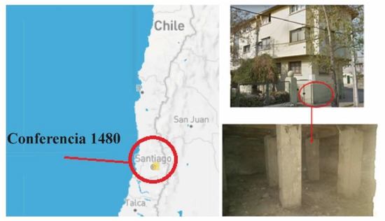
Figure 1.
One of the locations referenced in the text is observed: the mezzanine, located at 1480 Conference Street, Santiago de Chile.
- The first building was ideal for the concentration of radon. The floor is a kind of light gravel located on a false floor, intended for thermal insulation, with minimal ventilation that was completely eliminated between hours 480 and 530 (peak concentration) and then returned to its initial condition. Its location is at Conference Street No. 1480 and the measurement period was from 30 October 2020, to 2 December 2020, Figure 2a.
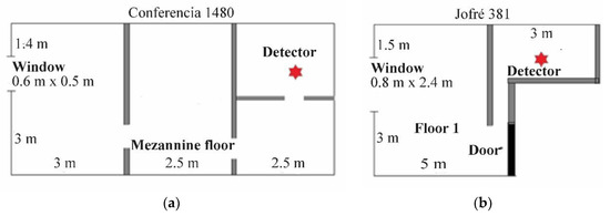
Figure 2.
Top view of the two locations for radon concentration measurements. (a). The floor of the house is a kind of light gravel located on a false floor, intended for thermal insulation with very little ventilation, a technique used in houses built more than 60 years ago. (b). The second house has characteristics similar to the first, a little better ventilated and smaller in size.
- The second building was more ventilated, so the radon concentrations were lower. It was used as a reference parameter for lower concentrations and another season of the year. The units are on the first floor, located at Jofré street No. 381. The measurement period was from 28 May 2021 to 12 July 2021. Figure 2b.
2.2. The Data
The detector, as shown in Figure 3, measures radon, temperature, relative humidity, atmospheric pressure, and angle of inclination (an indicator that shows if a detector moves between measurements). It has data acquisition software that allows graphical analysis of the information, called CRA PC Software Corentium Report Analysis (Cra software version 4.5v Corentium Report and analysis creation date 9 March 2020, Norway, Wergelandsveien 7, 0167 Oslo, www.airthings.com (accessed on 19 May 2020).
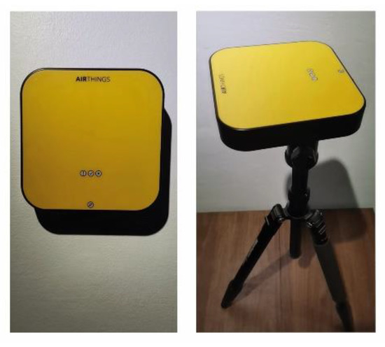
Figure 3.
Corentium Pro Detector, used to measure Radon concentration and meteorological variables.
Corentium Pro detector, serial number 2700009022, Manufacturer Airthings A.S. manufacturing city, Norway, Wergelandsveien 7, 0167 Oslo.
The Corentium Pro meter samples indoor air in a passive diffusion chamber and, using alpha spectrometry, accurately calculates Radon levels. Thanks to its silicon photodiodes, it detects radon to count and measure the energy of the alpha particles resulting from the radon decay chain. Its calibration is carried out with reference instruments in authorized laboratories, and it is certified by the AARST (The American Association of Radon Scientists and Technologists)-NRPP (National Radon Proficiency Program), and NRSB (National Radon Safety Board).
The standard deviation from exact radon levels is less than 7% + 5 Bq/m3 after 24 h and less than 5% + 2 Bq/m3 after 7 days. The Radon measurement protocol is ISO 11665-1:2019 and ISO 11665-5:2020.
The data accumulation capacity exceeds periods of 2 years. Once the monitoring is finished, the data is entered into an analysis platform through a Hub. If all the protocols and certifications are met, this data becomes part of the world radon map, developed by the company Airthings.
2.3. Methodology Applied in the Analysis of Non-Linear Time Series
2.3.1. Kolmogorov Entropy and Its Relation to Information Loss
According to Farmer, one of the essential differences between chaotic and predictable behavior is that chaotic trajectories continuously generate new information while predictable trajectories do not [18,19]. Metric entropy makes this notion more rigorous. In addition to providing a good definition of chaos, metric entropy provides a quantitative way to describe how chaotic a dynamical system is. In the Kolmogorov entropy [20], SK is the average loss of information [21,22,23] when “l” (side of the cell in units of information) and τ (time) become infinitesimal:
SK has units of information bits per second and bits per iteration in the case of a discrete system [24,25]. The limit process of Equation (1), follows the order: (i) n → ∞, (ii) l → 0, canceling the dependency of the selected partition (n is the number of cells or partitions) and (iii) τ → 0, for continuous systems. The Kolmogorov entropy difference, ΔSK = SKn +1 − SKn between two neighboring cells, gives the required complementary information about the cell (in + 1) in which the system will be in the future. The difference gives the loss of information, in time, of the system.
In summary, for the calculation of the Kolmogorov entropy, it is first verified that the entropy is between zero and infinity (0 < SK < ∞), which allows for verifying the presence of chaotic behavior. If the Kolmogorov entropy is equal to 0, no information is lost, and the system is regular and predictable. If SK = ∞, the system is completely random, and it is impossible to make any predictions. Second, the amount of information required to predict the future behavior of two interacting systems, in this case, the atmosphere and hourly concentration of Radon, is determined. In this way, the rate at which the system loses (or outdates) information over time can be estimated. Finally, the horizon of maximum predictability of the system can be established. This horizon is a limited frontier from which it is not possible to make predictions or formulate new scenarios [15]. The loss of information can be determined according to the equation:
λ is the Lyapunov exponent, <ΔI> in [bits/hr], is the loss information. Two types of <ΔI> were calculated: one for the contribution of Radon, and another for the sum of the loss of information of each meteorological variable (MV): temperature (T), pressure (P), and relative humidity (HR).
In this study, the set of localized measurements belonging to meteorological variables was selected for comparison with other investigations that use them, and of Radon concentration, measurements that form time series. Software [26,27] was applied that allows analyzing the chaotic nature of each time series. Once its chaoticity has been verified, the calculation of the entropy flows, (∂S⁄∂t), allows us to analyze the information and characterize its interaction.
2.3.2. Nonlinear Time Series Analysis Elements
There are many investigations of nonlinear time series [28,29,30]. It is common for these studies to start with the calculation, through Taken’s method [31], of (i) the delay time (τ) using the average mutual information [30] and (ii) the embedding dimension, m (also written dc) that applies the false nearest neighbor’s technique [28,32,33].
In nonlinear analysis, we also use: the dimension of correlation, Dc [27], the Hurst exponent, H [34], the entropy of correlation, K2. and the Kolmogorov entropy, SK. One of the essential chaotic indicators is the Lyapunov exponent, λ [33], defined [28] as:
where n is the number of iterations. This means that if two points of an orbit, in the beginning, are very close, λ is determined for a large value of n. If after n iterations the points separate, it is a sign of the probable presence of chaos in the system. Finding a maximum positive value of λ indicates chaos in the time series [35,36]. The sum of all λ > 0, determined from the time series, defines its SK entropy and allows us to calculate, approximately, the average predictability time TA = 1/SK [28]. From a practical point of view, λ is obtained from Equation (3) in the limit for large n that makes saturation manifest. This is what motivates working with time series containing over 5000 data points [37] (another reason points to stability conditions in the calculation). The correlation entropy of the time series, K2 [27,38] is defined as:
where n is the number of points –or data-, m is the embedding dimension and r is the radius of the circle or hypersphere and is such that it can produce the values: 0 (regular data), greater than 0 (chaotic data), ∞ (random data). Kolmogorov entropy, in the same way as K2, indicates whether a time series of experimental data is regular, chaotic, or random, a criterion used with respect to Radon time series and meteorological variables.
In Equation (4), C (m, r) is the correlation sum of the reconstructed path of a time series. A method to estimate K2 is based on Grassberger and Procacia [34]. In this studio, the Kolmogorov entropy, SK, has been calculated for each of the measured time series of Radon and meteorological variables in the different seasons of the year. C (m, r) is the correlation sum for a given embedding dimension m and is used to estimate the correlation dimension [27], defined from:
where (the superscript of the sum depends on the embedding dimension (m)), C(r) is the correlation integral (the number of points within all circles of radius r normalized to 1, when r is large enough to include all points without double counting); n is the number of data; H is the Heaviside function, ‖…‖ denotes the norm or distance between two vectors, the Euclidean distance gives more robust results in the presence of noise, where r is a real number that should be chosen with caution, since small values of r mean that C(r) is meaningless, and for large values of r, C(r) does not give relevant information. Equation (5) can be written as:
C(r) is calculated by varying r from 0 to the largest possible value of . For sufficiently small values of r and for a very large amount of data, C(r) behaves according to a power law of the type:
DC is the correlation dimension (or correlation exponent). From Equation (6) and taking the logarithm of both sides, we see that DC is obtained by plotting log C(r) vs. log r. It is observed that, if DC does not saturate at some value as m increases, the process is random (or stochastic). Otherwise, if DC saturates at some value, the time series is said to be rather deterministic [39]. In our study, for the six time-series, DC was saturated at values given in Table 1. One dimension of correlation, DC > 5 implies –essentially- random data, which does not occur in this study. One of the objectives of this study is to examine the behavior (deterministic, chaotic, or random) of the radon time series and of three time-series of meteorological variables (pressure, relative humidity, and temperature). However, this study demonstrates that radon concentration time series are chaotic. The same happens for time series of meteorological variables. The most important indices (or metric quantities) in nonlinear time series analysis are: lag time, τ; lace dimension, m; maximum positive Lyapunov exponent, λ; correlation dimension, DC; Kolmogorov entropy SK and the Hurst exponent, H, which allow the chaoticity of the system to be quantified. So, if the correlation dimension is below 5.0, the Lyapunov exponent is positive, and the Kolmogorov entropy has a finite and positive value, then chaos would be present in the time series under study. The Kolmogorov SK entropy characterizes the degree of chaos for a nonlinear system. This value is proportional to the information loss rate of the system.

Table 1.
Chaotic parameters, periods 30 October 2020 to 2 December 2020, and 28 May 2021 to 12 July 2021.
The Lyapunov exponent, λ, defines the nature of the time evolution of nearby orbits in phase space and is considered an essential component of chaotic behavior. The correlation entropy, K2, is a lower limit of the Kolmogorov entropy, SK [38]. Following the preceding considerations, it is possible to indicate:
It is also possible to analyze the time series from another point of view, using the Hurst Exponent, H. Through the fractal dimension, D = 2 − H, the roughness of the time series is analyzed, allowing to describe objects that present a high degree of complexity, comparing them according to the study periods. If 0.5 < H < 1, these are time series that present persistence (long-term memory effects). Theoretically, what happens in the present will affect the future forever, and all current changes are correlated with all future changes. In the case of the present study, it means that the time series are persistent, since for every Hurst exponent it is greater than 0.5 and less than 1.
The presented mathematical formalism has a numerical calculation software that allows us to analyze the experimental time series of radon and the meteorological variables, each one without missing data. The applied numerical procedure, based on chaos theory [23,27,39], also has the data analysis method called fragmentation test for iterated function systems (IFS). The method uses symbolic dynamics [40] and allows us to calculate the Lempel-Ziv complexity (LZ) relative to white noise. The presence of chaotic data is manifested graphically by the distribution of clumpiness of points on the surface. The series of this study comply with 0 < LZ < 1. The summary of the relevant chaotic parameters calculated is shown in Table 1.
3. Results
The results shown in Table 1 were obtained by processing the data with chaotic time series analysis software [26]. Symbols used: λ: Lyapunov exponent; Dc = Correlation Dimension; SK = Entropy of Correlation; LZ = Lempel Complexity − Ziv; H = Hurts exponent; τ = predictability time; D = fractal dimension = 2 − H.
This study considers the construction of a ratio between the entropy of the time series of each meteorological variable and the entropy of the time series of the radon activity level. The quotient allows us to analyze the effect of urban meteorology on the concentration of Radon according to the seasons spring–summer and autumn–winter, as shown in Table 2.
Table 2.
Quotients between the entropy of the radon concentration and the meteorological variables for the spring–summer (Series 1) and autumn–winter (Series 2) periods.
The loss of information was determined for the time series of the meteorological variables and the level of radon activity. The loss of information allows us to estimate and compare, very approximately, the predictability time according to the spring–summer and autumn–winter seasons, shown in Table 3.
Table 3.
<ΔI> in [bits/hr] (Equation (2)): loss information as the sum of the contribution of P (Pollution:radon) and the sum of the contribution of each MV(Meteorological Variables: T, P, RH).
According to the data, in the 28 May 2021–12 July 2021 period (autumn–winter), the new information generated is close to the old information, and the entropy of the radon gas is lower, increasing the predictability time. The System is less chaotic. In the period 30 October 2020–2 December 2020, the new information generated is far from the old information, the entropy of radon is higher, and its predictability time is lower. The System is more chaotic. The meteorological variables for the period 28 May 2021–12 July 2021 lose information slowly, acting as a barrier, which favors the decay of the radon concentration. While in the period 30 October 2020–2 December 2020, the meteorological variables lose information faster, favoring the growth of the radon concentration.
The graphs of the entropy ratio of the meteorological variables and radon concentration are presented below, Figure 4, by the season of the year:
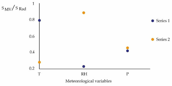
Figure 4.
It represents the quotient between the entropy of the radon concentration (SRad) and the meteorological variables (SVM) for the Spring-Summer (Series 1) and Autumn-Winter (Series 2) periods.
30 October 2020–2 December 2020, Spring–Summer
Figure 5 presents the concentration of Radon in the spring–summer period:
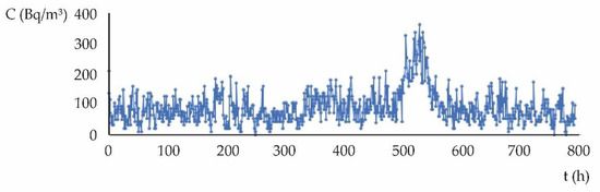
Figure 5.
Evolution of the hourly concentration of radon (spring–summer). The highest points of radon concentration correspond to a short period (1 day) of total closure of the measurement zone.
Figure 6 presents the Hurst coefficient (persistence indicator) for each study variable:
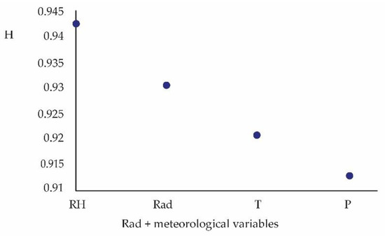
Figure 6.
Persistence, H, versus radon (Rad) plus meteorological variables of the study, spring–summer period, data extracted from Table 1.
The Lempel-Ziv complexity tells us if it is possible to find new data subsequences within each time series, which increases the complexity counter. Figure 7 presents LZ for each time series of the study:
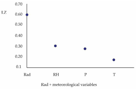
Figure 7.
Lempel Ziv Complexity, LZ, versus study variables. Data extracted from Table 1.
High temperatures and porous structures are important factors affecting the radon emission rate in rocks [41]. Other investigations [42] indicate that the impact of the interior-exterior temperature difference was not statistically significant on the radon concentration. In this study of the interior of a House, the values of persistence and complexity of Lempel-Ziv for temperature are low (Figure 5 and Figure 6), for the spring—summer period. The entropy of the temperature time series is lower in winter compared to that of Radon. Winter temperatures, on average, are lower. The reverse occurs in the warmer season or higher temperatures (Series 1, Figure 4). The entropy of the temperature time series is lower, of the order of 20.4%, compared to that of Radon. This favors the concentration of Radon, which is confirmed by its complexity and persistence (Figure 5 and Figure 6).
20 May 2021–21 July 2021, Autumn–winter
Figure 8 presents the concentration of Radon in the autumn–winter period:
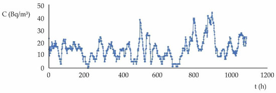
Figure 8.
Radon concentration hourly variation (Autumn–winter measurements).
Figure 9 presents the Hurst coefficient (persistence indicator) for each study variable:
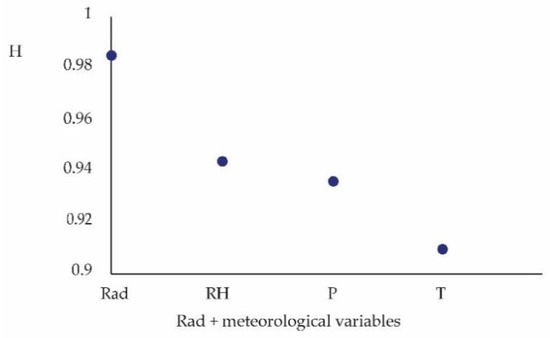
Figure 9.
Hurst and Rad coefficient, plus meteorological variables, according to the data extracted from Table 1.
Figure 7 presents LZ for each time series of the study:
Figure 10 shows that the relative humidity of the autumn–winter period is more complex compared to the radon concentration time series, however, the latter is more persistent (Figure 9). It can be stated that relative humidity moderates the radon concentration in its connectivity with the environment, according to Figure 10.
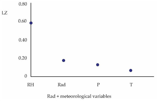
Figure 10.
Lempel-Ziv complexity, and Rad, plus meteorological variables (Table 1).
4. Discussion
From the data log, the average seasonal values of radon concentration are obtained:
for the autumn–winter period (normal passive ventilation), measurement period 44 days
Bq/m3, for the spring–summer period (low ventilation), measurement period 30 days, and
Bq/m3, spring–summer (without ventilation), for a period of 3 days. This shows the high impact that closed spaces have on the concentration of radon.
Figure 4 reveals the strong seasonality of radon concentrations, since it is the temperature in the spring–summer period that contributes to bringing the system to its state of the highest probability -close to equilibrium- environmental condition. This favors the highest concentration of said gas, which is indicated by the average value of the concentration in the spring–summer period. This does not occur in the measurements of the autumn–winter period, since only the relative humidity variable pushes the system to equilibrium. But this is not enough to make the radon concentration sustainable. The predictability times are comparable in the spring–summer period for the temperature meteorological variable. This gives a probable time of sustainability to the radon concentration, in the vicinity of its predictability time. The predictability times for the relative humidity meteorological variable, in the autumn–winter period, are of the order of the radon time. But relative humidity does not favor its concentration, and does not contribute to its sustainability, as shown in Figure 3, according to series 1 (spring—summer) and series 2 (autumn—winter).
The average values for temperature and relative humidity are the following, for the two periods measured: Spring—summer: = 21.1 °C, = 64.7%; autumn—winter: = 16.3 °C, = 55.09%.
The values obtained for the Lyapunov exponents (λ > 0), Hurst exponent (0.5 < H < 1.0), and correlation dimension (Dc < 5), and shown in Table 1, allow ruling out random behavior. This allows us to conclude that the time series is chaotic and very sensitive to the initial conditions. The radon concentration time series responds to a process with dissipative and irreversible characteristics (λ > 0, SK > 0) to the extent that its emission, and the associated energy, continue to invade the atmosphere, within the boundary layer, in this studio. The IFS (Iterated Function Systems) fragmentation test also suggests a method of data analysis. Through the use of symbolic dynamics [40], we can calculate the Lempel-Ziv complexity (LZ > 0, chaotic series) relative to white noise. When the data are chaotic, they are distributed forming, on a surface, localized groups, which was confirmed for the meteorological variables and radon in this study. The Kolmogorov entropy SK characterizes the degree of chaos for a nonlinear system. This value is proportional to the rate of loss of system information (Table 1, fourth column (SK)).
The spaces located below the surface level and lower floors adjacent to the surface, and with low ventilation -measurement points-, show high levels of radon concentration. Figure 6 and Figure 7 indicate that the radon concentration and relative humidity have the highest persistence and the highest Lempel-Ziv complexity. This would indicate that even in the spring–summer seasons, relative humidity plays an important role in the concentration of radon in closed spaces. However, Figure 3 indicates that, according to the entropy ratio, the effect of temperature in the spring–summer seasons is the most significant [13]. Figure 9 and Figure 10 show that in the autumn–winter period, radon has the highest persistence (H) and relative humidity has the highest Lempel-Ziv complexity. Temperature shows minima for both the H and LZ plots.
By dividing the entropy of each meteorological variable, considered in this study, by the entropy of radon gas, it is obtained that the quotient is less than 1. This implies that radon is more dominant, with respect to the meteorological variables, in both periods seasonal.
Figure 4 shows the ratio between the radon concentration entropy and the entropies of the meteorological variables, observing that in winter, the meteorological variable that most influences the concentration of radon is relative humidity. And it is complex and persistent, which attenuates the effect of radon [12,13]. In summer, the relative humidity entropy is mediated by the radon concentration in the closed measurement space and tends to decrease (see Table 1). The pressure, according to the chaotic analysis, has an effect on the radon concentration [14], as indicated in Figure 4, and brings it to a certain equilibrium, independent of the season. In the autumn–winter period, the fractal dimension (D) is lower compared to that of the spring–summer period. This gives a qualitative weighting of the effect of meteorology on radon. This attribute is related to the degree of roughness that the time series presents, and allows us to mathematically describe objects that present a high degree of complexity, self-similarity, or chaos. That is, the system under study is more chaotic in the spring–summer period (Table 1). The chaotic analysis confirms the behavior of radon in the presence of significant meteorological variables, temperature, and relative humidity, indicated according to other approaches [12,13,14].
5. Conclusions
The application of the tool for chaotic analysis to the treatment of radon concentration time series confirms its chaoticity ( with fractal dimension). The time series of the measured meteorological variables (temperature, relative humidity, and environmental pressure) are chaotic [43] in a relatively short period (one month and one month and fraction), showing that even in that period they also play an effective role on radon concentration levels. All the series, moreover, represent irreversible processes that, through comparable predictability times between some meteorological variables with that of the radon concentration, exhibit the sensitivity of radon to specific meteorological variables. It is demonstrated from the analysis of the entropy ratio, between the meteorological variables and the radon concentration, that the relative humidity plays an important seasonal role (within the year) on the concentration levels of radon gas: by itself, it attenuates it in the autumn–winter period. In the spring–summer period, the temperature favors the concentration of radon. On the other hand, the ratio between the environmental pressure entropy and the radon concentration shows some stability, in the order of 50%, regardless of the season of the year. This allows us to assert that the pressure would tend to favor the permanence of radon, according to the urban measurements carried out in this study.
These types of measurements, which are preliminary and scarce in Chile, prove that it is adequate and necessary to monitor radon from the perspective of industrial construction, housing, etc., that have low ventilation and prolonged use by the population [10]. According to seasonal average values: 15.5 Bq/m3 autumn–winter, measurement period 44 days.
92.2 Bq/m3 spring–summer, measurement period 33 days, and applying Table 1, this research reveals that the average value of the spring–summer period is high, which is supported by the seasonal urban weather [3]. This could be indicating that there is an annualized average rate above the values estimated as adequate for radon measurements and analysis, in the study areas [9,10]. This last conclusion warrants extending this investigation. Finally, from the application of chaos theory, results are obtained that show very good agreement with the data and interpretations made through other mathematical formalisms.
Author Contributions
Conceptualization, P.P.; methodology, P.P. and H.U.; software, P.P.; validation, P.P., H.U. and E.M.; formal analysis, P.P.; investigation, P.P, H.U. and E.M.; resources, E.M.; data curation, H.U; writing—original draft preparation, P.P.; writing—review and editing, P.P. and H.U.; visualization, H.U. and E.M.; supervision, P.P.; project administration, P.P.; funding acquisition, P.P. All authors have read and agreed to the published version of the manuscript.
Funding
Project supported by the Competition for Research Regular Projects from the year 2020, code LPR20-02, Universidad Tecnológica Metropolitana.
Institutional Review Board Statement
Not applicable.
Informed Consent Statement
Informed consent was obtained from all subjects involved in the study.
Data Availability Statement
The data were obtained from the public network for online monitoring of meteorological variables. The network is distributed throughout Chile, without access restrictions. It is under the responsibility of SINCA, the National Air Quality Information System, dependent on the Environment Ministry of Chile. The data of the concentration of Radon for the two periods of the study were measured by one of the authors of the investigation, Mr. Héctor Ulloa A.
Acknowledgments
To the Research Directorate of the Universidad Tecnológica Metropolitana that made possible the progress of this research.
Conflicts of Interest
The authors declare no conflict of interest.
References
- Foken, T. Micrometeorology; Springer-Verlag Berlin Heidelberg: Berlin/Heidelberg, Germany, 2008. [Google Scholar] [CrossRef]
- Mauree, D.; Coccolo, S.; Deschamps, L.; Loesch, P.; Becquelin, P.; Scartezzini, J.L. Mobile Urban Micrometeorological Monitoring (MUMiM). J. Phys. Conf. Ser. 2019, 1343, 012014. [Google Scholar] [CrossRef]
- Stull, R.B. Introduction to Boundary Layer Meteorology; Kluwer Academic: Dordrecht, The Netherlands, 1988; p. 666. [Google Scholar]
- Klausner, Z.; Ben-Efraim, M.; Arav, Y.; Tas, E.; Fattal, E. The Micrometeorology of the Haifa Bay Area and Mount Carmel during the summer. Atmosphere 2021, 12, 354. [Google Scholar] [CrossRef]
- Fattal, E.; David-Saroussi, H.; Klausner, Z.; Buchman, O. An Urban Lagrangian Stochastic Dispersion Model for Simulating Traffic Particulate-Matter Concentration Fields. Atmosphere 2021, 12, 580. [Google Scholar] [CrossRef]
- Garratt, J.R.; Pearman, G.I. Retrospective Analysis of Micrometeorological Observations Above an australian wheat crop. Bound. Layer Meteorol. 2020, 177, 613–641. [Google Scholar] [CrossRef]
- Park, J.H.; Lee, C.M.; Lee, H.Y.; Kang, D.R. Estimation of Seasonal Correction Factors for Indoor Radon Concentrations in Korea. Int. J. Environ. Res. Public Health 2018, 15, 2251. [Google Scholar] [CrossRef]
- Yanchao, S.; Bing, S.; Hongxing, C.; Yunyun, W. Study on the effect of air purifier for reducing indoor radon exposure. Appl. Radiat. Isot. 2021, 173, 109706. [Google Scholar] [CrossRef]
- Organización Mundial de la Salud. Manual de la OMS Sobre el Radón en Interiores. Una Perspectiva de Salud Pública; Organización Mundial de la Salud: Geneva, Switzerland, 2015; ISBN 978-92-4-354767-1. Available online: https://apps.who.int/iris/bitstream/handle/10665/161913/9789243547671_spa.pdf (accessed on 3 September 2021).
- Gaskin, J.; Coyle, D.; Whyte, J.; Krewksi, D. Global Estimate of Lung Cancer Mortality Attributable to Residential Radon. Environ. Health Perspect. 2018, 126, 057009. [Google Scholar] [CrossRef]
- Minvu. Estándares de Construcción Sustentable Para Viviendas, Tomo I: Salud y Bienestar; Ministerio de Vivienda y Urbanismo: Santiago, Chile, 2018; ISBN 978-956-9432-52-1. Available online: https://csustentable.minvu.gob.cl/wp-content/uploads/2018/03/EST%C3%81NDARES-DE-CONSTRUCCI%C3%93N-SUSTENTABLE-PARA-VIVIENDAS-DE-CHILE-TOMO-I-SALUD-Y-BIENESTAR.pdf (accessed on 2 October 2021).
- Singh, K.; Singh, M.; Singh, S.; Sahota, H.S.; Papp, Z. Variation of radon (222Rn) progeny concentrations in outdoor air as a function of time, temperature, and relative humidity. Radiat. Meas. 2005, 39, 213–217. [Google Scholar] [CrossRef]
- Akbari, K.; Mahmoudi, J.; Ghanbari, M. Influence of indoor air conditions on radon concentration in a detached house. J. Environ. Radioact. 2013, 116, 166–173. [Google Scholar] [CrossRef]
- Baltrenas, P.; Grubliauskas, R.; Danila, V. Seasonal Variation of Indoor Radon Concentration Levels in Different Premises of a University Building. Sustainability 2020, 12, 6174. [Google Scholar] [CrossRef]
- Kolmogorov, A.N. On Entropy per unit Time as a Metric Invariant of Automorphisms. Dokl. Russ. Acad. Sci. SSSR 1959, 124, 754–755. [Google Scholar]
- Rafique, M.; Iqbal, J.; Shah, S.A.A.; Alam, A.; Lone, K.J.; Barkat, A.; Shah, M.A.; Qureshi, S.A.; Nikolopoulos, D. On fractal dimensions of soil radon gas time series. J. Atmos. Sol. Terr. Phys. 2022, 227, 105775. [Google Scholar] [CrossRef]
- Dimitrios, N.; Christos, M.; Panayiotis, Y.H.; Ermioni, P.; Demetrios, C.; Constantinos, N. Long-Memory and Fractal Trends in Variations of Environmental Radon in Soil: Results from Measurements in Lesvos Island in Greece. J. Earth Sci. Clim. Chang. 2018, 9, 4. [Google Scholar] [CrossRef]
- Farmer, J.D. Chaotic attractors of an infinitedimensional dynamical system. Physica D 1982, 4, 366–393. [Google Scholar] [CrossRef]
- Farmer, J.D.; Otto, E.; Yorke, J.A. The dimension of chaotic attractors. Physica D 1983, 7, 153–180. [Google Scholar] [CrossRef]
- Martínez, J.A.; Vinagre, F.A. La Entropía de Kolmogorov; su Sentido Físico y su Aplicación al Estudio de Lechos Fluidizados 2D; Departamento de Química Analítica e Ingeniería Química, Universidad de Alcalá: Alcalá de Henares/Madrid, Spain, 2016; Available online: https://www.academia.edu/2479372 (accessed on 19 July 2019).
- Shannon, C. A mathematical theory of communication. Bell Syst. Tech. J. 1948, 27, 379–423, 623–656. [Google Scholar] [CrossRef]
- Brillouin, L. Science and Information Theory, 2nd ed.; Academic Press: New York, NY, USA, 1962; 304p. [Google Scholar]
- Pacheco, P.R.; Salini, G.A.; Mera, E.M. Entropía y Neguentropia: Una Aproximación al Proceso de Difusión de Contaminantes y su Sostenibilidad. Rev. Int. Contam. Ambient. 2021, 37, 167–185. [Google Scholar] [CrossRef]
- Shaw, R. Strange attractors, chaotic behavior and information flow. Z. Nat. A 1981, 36, 80–112. [Google Scholar] [CrossRef]
- Cohen, A.; Procaccia, I. Computing the Kolmogorov entropy from time signals of dissipative and conservative dynamical systems. Phys. Rev. A Gen. Phys. 1985, 31, 1872–1882. [Google Scholar] [CrossRef] [PubMed]
- Sprott, J.C. Chaos Data Analyzer Software. 1995. Available online: http://sprott.physics.wisc.edu/cda.htm (accessed on 1 March 2022).
- Sprott, J.C. Chaos and Time-Series Analysis; Oxford University Press: Oxford, UK, 2003; p. 528. [Google Scholar]
- Salini, G.; Pérez, P. A study of the dynamic behavior of fine particulate matter in Santiago, Chile. Aerosol Air Qual. Res. 2015, 15, 154–165. [Google Scholar] [CrossRef]
- Kumar, U.; Prakash, A.; Jain, V.K. Characterization of chaos in air pollutants: A Volterra-Wiener-Korenberg series and numerical titration approach. Atmos. Environ. 2008, 42, 1537–1551. [Google Scholar] [CrossRef]
- Fraser, A.M.; Swinney, H.L. Independent coordinates for strange attractors from mutual information. Phys. Rev. A 1986, 33, 1134–1140. [Google Scholar] [CrossRef]
- Takens, F. Detecting strange attractors in turbulence. In Dynamical Systems and Turbulence, Warwick (1980); Rand, D.Y., Young, L.S., Eds.; Springer: Berlin/Heidelberg, Germany, 1981; pp. 366–381. [Google Scholar]
- Salini, G.; Pérez, P. Estudio de series temporales de contaminación ambiental mediante técnicas de redes neuronales artificiales. Ingeniare 2006, 14, 284–290. [Google Scholar]
- Eckmann, J.P.; Oliffson, S.; Kamphorst, S.; Ruelle, D.; Ciliberto, C. Lyapunov exponents from time series. Phys. Rev. A 1986, 34, 4971–4979. [Google Scholar] [CrossRef]
- Grassberger, P.; Procaccia, L. Characterization of strange attractors. Phys. Rev. Lett 1983, 50, 346–349. [Google Scholar] [CrossRef]
- Kantz, H.; Schreiber, T. Nonlinear Time Series Analysis, 2nd ed.; Cambridge University Press: Cambridge, UK, 2004; p. 387. [Google Scholar]
- Sivakumar, B.; Wallender, W.; Horwath, W.; Mitchell, J. Nonlinear deterministic analysis of air pollution dynamics in a rural and agricultural setting. Adv. Complex Syst. 2007, 10, 581–597. [Google Scholar] [CrossRef]
- Wolf, A.; Swift, J.B.; Swinney, H.L.; Vastano, J.A. Determining Lyapunov exponents from a time series. Physica D 1985, 16, 285–317. [Google Scholar] [CrossRef]
- Gao, J.; Cao, Y.; Hu, J. Multiscale Analysis of Complex Time Series; Wiley and Sons Interscience: Hoboken, NJ, USA, 2007; 368p. [Google Scholar]
- Chelani, A.; Devotta, S. Nonlinear analysis and prediction of coarse particulate matter concentration in ambient air. J. Air Waste Manag. Assoc. 2006, 56, 78–84. [Google Scholar] [CrossRef][Green Version]
- Horna, J.; Dionicio, J.; Martínez, R.; Zavaleta, A.; Brenis, Y. Dinámica Simbólica y Algunas Aplicaciones. Sel. Mat. 2016, 3, 101–106. [Google Scholar] [CrossRef]
- Li, P.; Sun, Q.; Tang, S.; Li, D.; Yan, T. Effect of heat treatment on the emission rate of radon from red sandstone. Environ. Sci. Pollut. Res. 2021, 28, 62174–62184. [Google Scholar] [CrossRef]
- Dicu, T.; Burghele, B.D.; Botoş, M.; Cucoș, A.; Dobrei, G.; Florică, Ș.; Grecu, Ș.; Lupulescu, A.; Pap, I.; Szacsvai, K.; et al. A new approach to radon temporal correction factor based on active environmental monitoring devices. Sci. Rep. 2021, 11, 9925. [Google Scholar] [CrossRef] [PubMed]
- Lee, C.K.; Lin, S.C. Chaos in air pollutant concentration (APC) time series. Aerosol Air Qual. Res. 2008, 8, 381–391. [Google Scholar] [CrossRef]
Publisher’s Note: MDPI stays neutral with regard to jurisdictional claims in published maps and institutional affiliations. |
© 2022 by the authors. Licensee MDPI, Basel, Switzerland. This article is an open access article distributed under the terms and conditions of the Creative Commons Attribution (CC BY) license (https://creativecommons.org/licenses/by/4.0/).