Multi-Channel Blind Restoration of Mixed Noise Images under Atmospheric Turbulence

Abstract

The imaging quality of astronomical or space objects is significantly degraded by atmospheric turbulence, photon noise, image sensor noise, and other factors. A multi-channel alternating minimization (MCAM) method is proposed to restore degraded images, in which multiple blurred images at different times are selected, and the imaging object and the point spread function are reconstructed alternately. Results show that the restoration index can converge rapidly after two iterations of the MCAM method when six different images are adopted. According to the analysis of the structure similarity index, the stronger the influence of turbulence and mixed noise, the higher the degree of image improvement. The above results can provide a reference for blind restoration of images degraded by atmospheric turbulence and mixed noises.

1. Introduction

The imaging quality of astronomical or space objects is severely degraded due to the combined effects of atmospheric turbulence, photon noise, mechanical vibration, and image sensor noise. The imaging process leads to the loss of crucial information in the image details, which increases the difficulty of object recognition and location. Adaptive optics technology [1,2,3] and image reconstruction [4,5,6] are two common methods to solve the optical imaging problem by atmospheric turbulence. Compared with adaptive optics technology, image restoration technology does not require expensive and complex wavefront detectors, controllers, and correctors, and is widely used to process degraded images. Briefly speaking, image correction is the process of denoising and deconvolution. Up to now, a variety of methods have been proposed and applied in image restoration, such as speckle-dependent imaging [7], lucky imaging [8], phase diversity method [9], and blind deconvolution algorithms. The reconstruction of speckle imaging requires a large number of reference samples and a lot of high-frequency information in statistical data. The recovery results by lucky imaging depend on the quality of the captured images and are only suitable for conditions of slight turbulence. Although the phase diversity method can be directly applied to extended objects and realize simultaneous reconstruction of the phase and the objects, the convergence speed is too slow to be used for real-time image reconstruction.

Unlike the speckle-dependent imaging, lucky imaging, or phase diversity method, the blind deconvolution algorithm does not require prior knowledge, especially suitable for the case where both the original object and the point spread function (PSF) are unknown. At the same time, it has low requirements for imaging systems. In the 1970s, Andrews and Hunt [10] developed a blind restoration algorithm based on a specific model, which opened the prelude to the blind restoration algorithm. Ayers et al. [11] proposed a single-channel iterative blind deconvolution method based on the non-negativity of the image, which can easily incorporate various image- and Fourier-domain constraints. However, the uniqueness and convergence properties of this method are uncertain. Molina et al. [12] proposed a blind deconvolution using a variational approach to approximate the posterior probability of the unknown image, blur, and hyperparameters, which regards autoregressions as prior distributions for both the image and blur and gamma distributions for the unknown parameters of the priors and the image information noise. Based on the previous work of others, Schulz developed a multi-channel blind deconvolution algorithm based on maximum likelihood estimation [13]. The convergence has been improved, but the type of noise is single, and the point spread function is not constrained. Therefore, there are certain limitations in practical applications. In addition, a novel method employing example-based machine learning techniques for modeling the space of PSFs is given in [14]. During an iterative blind deconvolution process, a prior term attracts the PSF estimates to the learned PSF space, and then solves the PSF quickly. Methods of machine learning have recently become a research hotspot in the field of image reconstruction.

To successfully restore the degraded images by atmospheric turbulence and mixed noise, we present a new image reconstruction method, MCAM (multi-channel alternating minimization), in which the degraded images collected at different times are used as different channels, and the imaging object and the point spread function are reconstructed alternately. In the paper, we study the number of channels required by the method, the algorithm convergence speed and the image restoration quality.

2. MC Image Restoration Theory

2.1. Principle of MC Blind Deconvolution Algorithm

In general, the observed images may be regarded as either deterministic or stochastic signals, blurred by linear or nonlinear processes and corrupted with additive or multiplicative noise. Mathematically, incoherent optical imaging can be expressed as:

$$g\left(x,y\right)=\left[h\left(x,y\right)\otimes u\left(x,y\right)\right]\ast n_p+n_g,$$

(1)

where $g\left(x,y\right)$,$h\left(x,y\right)$ and $u\left(x,y\right)$ represent the degraded image, the PSF of the system and the original object, respectively. $n_p$ and $n_g$ are Poisson noise and Gaussian noise, respectively, and $\otimes$ is the convolution operator.

When converted into a matrix operation, Equation (1) can be expressed as:

$$G\left(x,y\right)=\left[H\left(x,y\right)\otimes U\left(x,y\right)\right]N_p+N_g$$

(2)

Equation (2) can be written as follows under no noise:

$$G\left(x,y\right)=\left[H\left(x,y\right)\otimes U\left(x,y\right)\right]$$

(3)

For two-channel imaging, Equation (4) can be obtained by mathematical transformation of Equation (3):

$$\left[G_2,-G_1\right]\left[\begin{array}{c}{H}_1^T\\ H_2^T\end{array}\right]=0$$

(4)

where G₁, G₂ represent the two different degraded images, and H₁, H₂ are corresponding PSFs. As seen in Equation (4), the object $U\left(x,y\right)$ is not contained in it. Since G₁, G₂ are known, the solution of H₁, H₂ has been transformed into a linear problem [14]. Similarly, for n > 2 the formula for n-channel imaging is as follows:

$$\{\begin{array}{c}\begin{array}{c}{G}_n{H}_{n-1}-G_{n-1}{H}_n=0\\ G_{n-1}{H}_{n-2}-G_{n-2}{H}_{n-1}=0\end{array}\\ ⋮\\ G_3{H}_2-G_2{H}_3=0\\ G_2{H}_1-G_1{H}_2=0\end{array}$$

(5)

In the case of no noise, PSFs can be solved according to Equations (4) and (5), and then the object’ parameters can be obtained by the classical deconvolution method. Mathematically, the premise of uniqueness of the solution to Equation (5) is that PSFs of different times satisfies the co-prime relationship. The previous results have proved this co-prime relationship [15]. However, imaging process is not only affected by atmospheric turbulence, but also suffers from noise. As a result, solving the PSF from the observed image becomes a mathematically ill-posed problem. In general, regularization methods are often adopted to constrain the range of the solution.

2.2. Solving Ill-Posed Problems

It can be seen from Section 2.1, the blind restoration of turbulence-degraded images evolves into solving an ill-posed problem because of noise corruption, which cannot estimate PSFs directly from observed images. Regularization is one of the most efficient methods for the solution of ill-posed problems. In [16], a mathematical model of an ill-posed problem is defined as follows:

$$\underset{u,\left\{h_k\right\}}{min}F\left(u,\left\{h_k\right\}\right)+Q\left(u\right)+R\left(\left\{h_k\right\}\right),$$

(6)

where $F\left(u,\left\{h_k\right\}\right)$ represents data fidelity item, which ensures that the restored image is consistent with the original image in terms of content. $Q\left(u\right)$ and $R\left(\left\{h_k\right\}\right)$ denote regularization terms for the object function and PSF, which can constrain the complexity of this type of problems.

$F\left(u,\left\{h_k\right\}\right)$ in Equation (6) can be described by the following equation:

$$F\left(u,\left\{h_k\right\}\right)=\frac{\gamma }{2}{\displaystyle \sum }_{k=1}^n\parallel u\otimes h_k-g_k\parallel {}^2,$$

(7)

where γ is the weight of the data fidelity item and $\parallel u\otimes h_k-g_k\parallel$ is $L_2$ norm, which can effectively avoid over-fitting of the model.

Based on the alternate minimization method [17], the solution of Equation (6) can be transformed into solving two sub-problems: “$Q-step$” and “$R-step$” denoted as Equations (8) and (9), respectively.

$$“Q-step”:\underset{u}{min}F\left(u,\left\{h_k\right\}\right)+Q\left(u\right),$$

(8)

$$“R-step”:\underset{\left\{h_k\right\}}{min}F\left(u,\left\{h_k\right\}\right)+R\left(\left\{h_k\right\}\right),$$

(9)

The global minimum can be solved by a local minimum of the sub-problems [16]. In addition, ALM [18] is introduced to ensure that the expectation of the global minimum can be achieved for each sub-problem. In order to enhance the robustness of the algorithm to noise, the Laplacian operator [19] is employed at the same time.

3. Experiment and Analysis

In this section, we test the performance of the proposed method by simulated experiments and make qualitative and quantitative analyses about certain key parameters playing an important part in its performance.

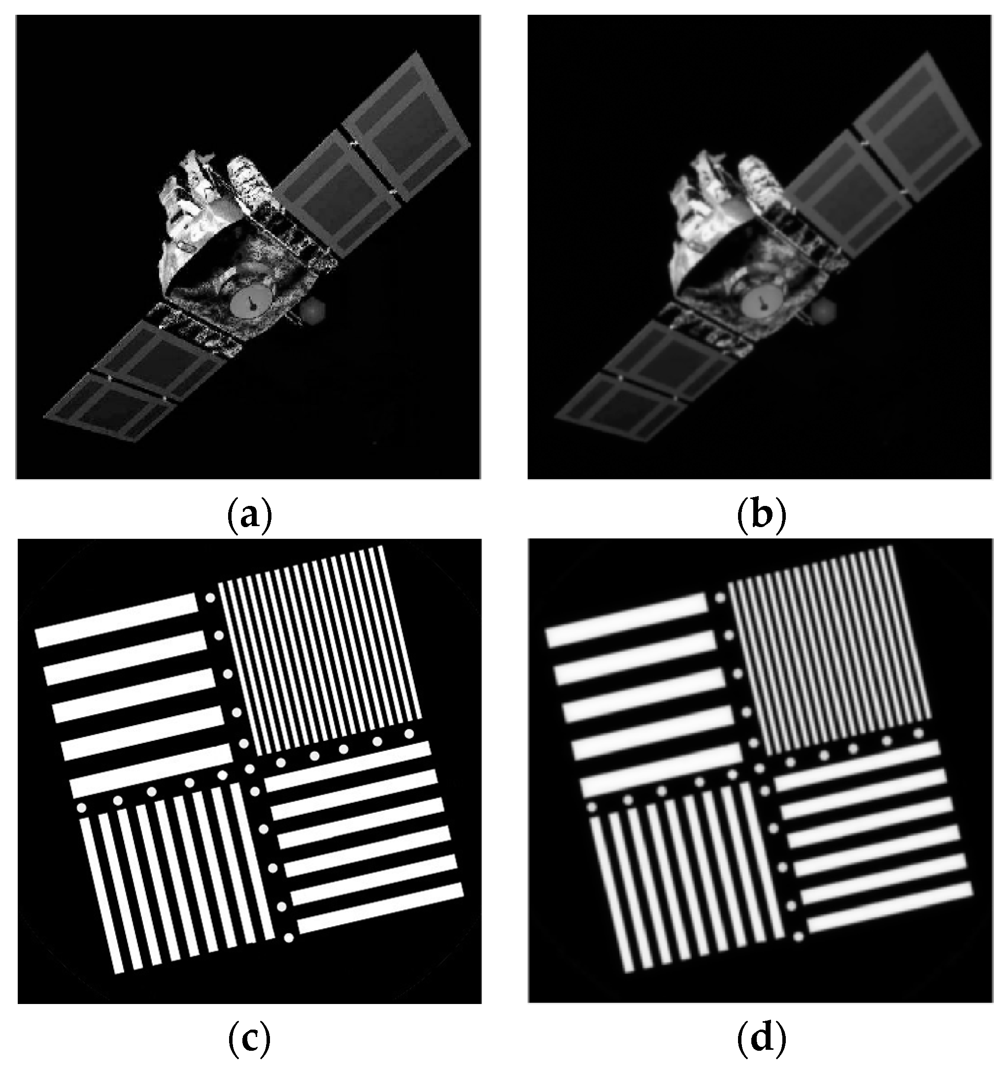
3.1. Experimental Environment

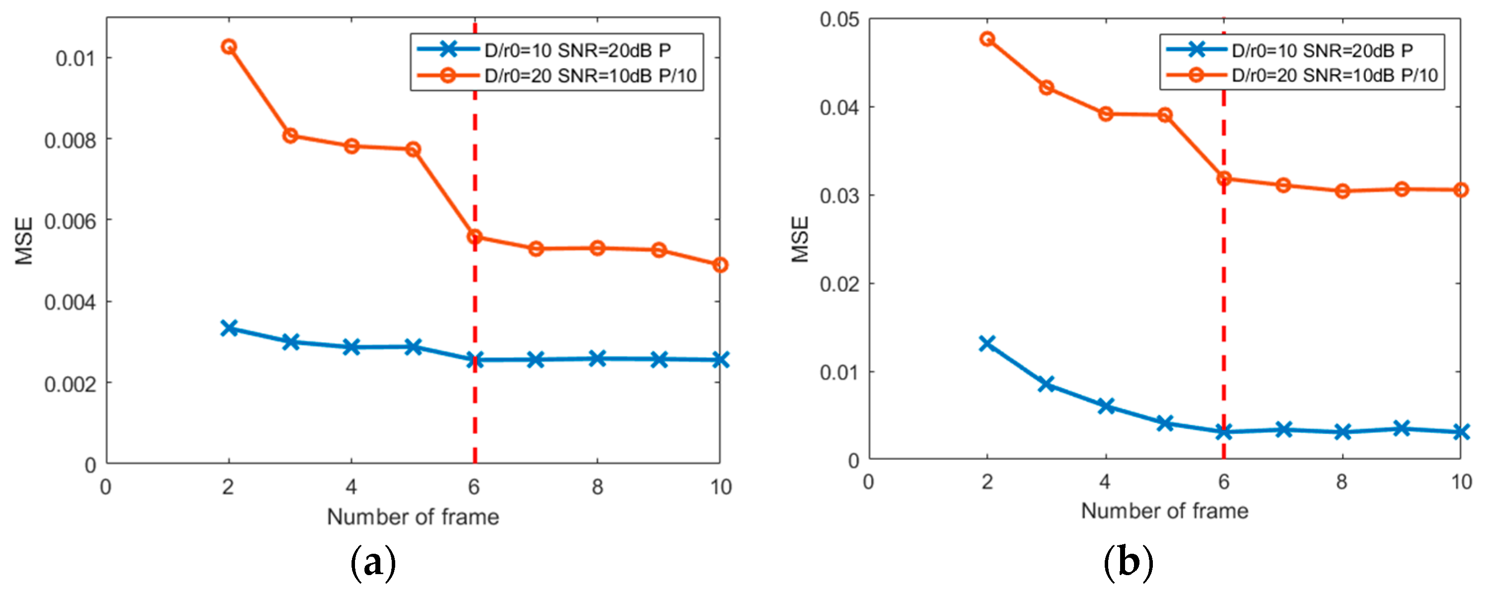
The Zernike polynomial of the randomly weighted Karhunen–Loève function [20] developed by Nicolas Roddier is used to describe the wavefront distortion affected by atmospheric turbulence.

In general, the influence of atmospheric turbulence on imaging can be characterized by D/r₀, where D is the telescope aperture size and r₀ is the atmospheric coherence length. When the aperture size D of the telescope remains unchanged, the smaller the atmospheric coherence length r₀, the greater the influence on the imaging. Generally, when the value of D/r₀ is greater than or equal to 20, atmospheric turbulence has an intense influence on imaging. When the value is less than 10, atmospheric turbulence has a weak effect on imaging. Other situations can be considered moderate influences. The imaging noise is the mixed noise, which is simulated by applying Gaussian noise and Poisson noise here. The Gaussian noise is represented by the signal-to-noise ratio (SNR) [21]. Poisson noise, also known as photon noise, is not a simple additive or multiplicative noise, and its pollution degree to the image is closely related to the degree of brightness or darkness [22]. The method in [23] is used to simulate the Poisson noise by changing the peak value of the imaging brightness.

In order to investigate the advantages of the MC alternating minimization method, we select the satellite image and the complex streak image as objects to be imaged (see Figure 1). Figure 1a,c are original objects, and Figure 1b,d are corresponding diffraction-limited imaging.

Figure 1. Objects to be imaged (a,c) and corresponding diffraction-limited imaging (b,d).

3.2. Channel Number

In this paragraph, we simulated a set of images according to model (2) with different parameters in order to discover the relationship between the number of channels or frames required and the quality of rebuilt images. For convenience, two sets of typical parameters with respect to atmospheric turbulence, Gaussian noise, and Poisson noise are selected. One is D/r₀ = 10, SNR = 20 dB, P, and the other is D/r₀ = 20, SNR = 10 dB, P/10. It is worth pointing out that the value of P is set to 255 when the bit depth of the grayscale image is 8. The smaller the peak value, the greater the intensity of Poisson noise.

The mean squared error (MSE) was used as the quality metric to quantitatively measure the image restoration performance. MSE is defined as follows:

$$MSE=\frac{1}{M}{\displaystyle \sum }_{m=1}^M{\left(Y_m-{\widehat{Y}}_m\right)}^2$$

(10)

where $Y_m$ is the reconstructed image and ${\widehat{Y}}_m$ is the diffraction-limited image.

Figure 2a,b show the relationship curves between the MSE and the number of channels for the satellite image and streak image, respectively. Each curve is obtained by the average result of 100 groups of degraded images under the same condition of the atmospheric turbulence level and mixed noise levels. From Figure 2, we can see that four MSE curves reach a relatively stable value when six frames of blurred images are used, and the greater the influence of turbulence, the stronger the noise, and the more noticeable this trend is. As the number of frames increases, the MSE does not decrease obviously while the amount of computation and the time consumed increase exponentially.

Figure 2. Relationship between MSE and the number of channels under different atmospheric turbulence and mixed noise. (a) Is for satellite and (b) is for stripe board.

We also conduct similar experiments on other different types of images under different turbulence and noise levels and obtain the same results. The above results show there is a good balance between the computation cost and the restoration effect when the six channels are selected.

The basic principle of six channels method is shown in Equation (11):

$$\left[\begin{array}{cccccc}0& 0& 0& 0& G_6& {-G}_5\\ 0& 0& 0& G_5& {-G}_4& 0\\ ⋮& & \ddots & & & ⋮\\ ⋮& & & \ddots & & ⋮\\ 0& G_3& {-G}_2& 0& 0& 0\\ G_2& {-G}_1& 0& 0& 0& 0\end{array}\right]\ast H=0$$

(11)

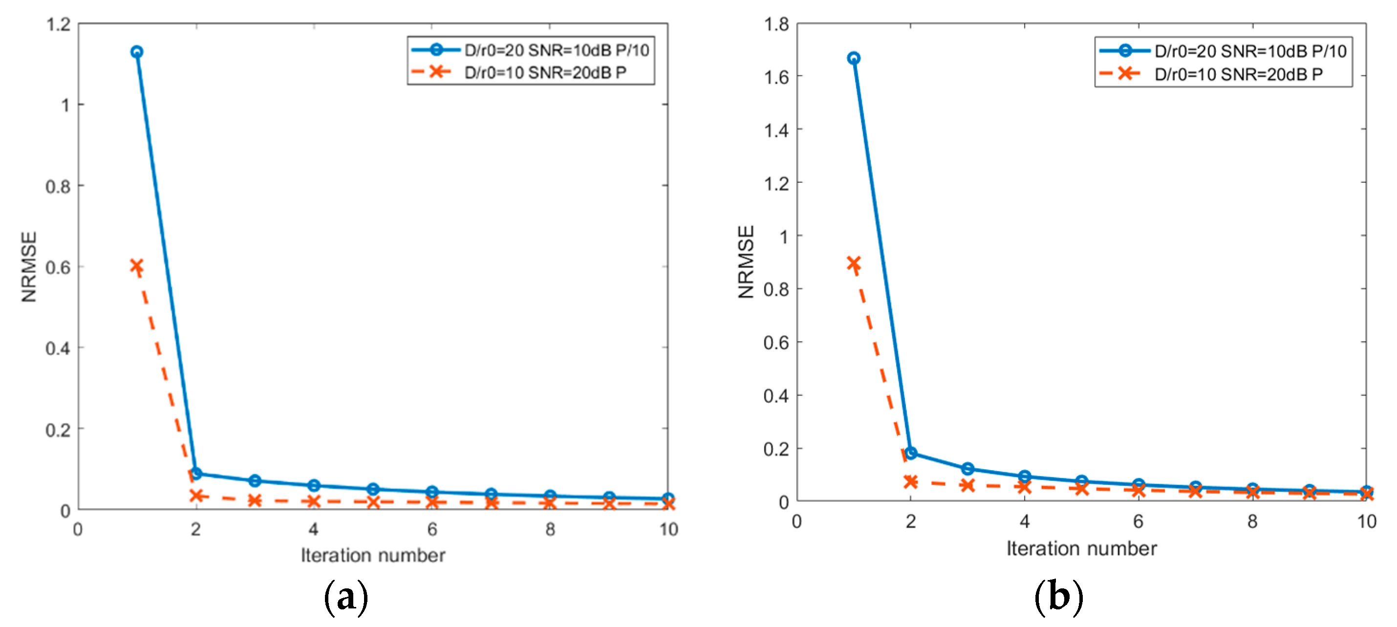
3.3. Convergence Speed of MCAM Method

To investigate the convergence speed of the MCAM method, we select six random blurred images under the same turbulence level and mixed noise to restore the PSF and the original object on the basis of the conclusion of Section 3.2. The convergence and convergent rates are analyzed by normalized root mean square error (NRMSE). The curves of NRMSE can describe the process from divergence to convergence more accurately and intuitively. Figure 3a,b show NRMSE curves of the six-channel MCAM method under different turbulence and mixed noise levels.

Figure 3. NRMSE curves of six-channel MCAM method. (a) Is for satellite and (b) is for stripe board.

As can be seen from Figure 3, the NRMSE value converges quickly after two iterations. This proves that the alternate minimization algorithms have fast convergence speeds and can converge close to the optimal performance under different atmospheric turbulence and mixed noise levels.

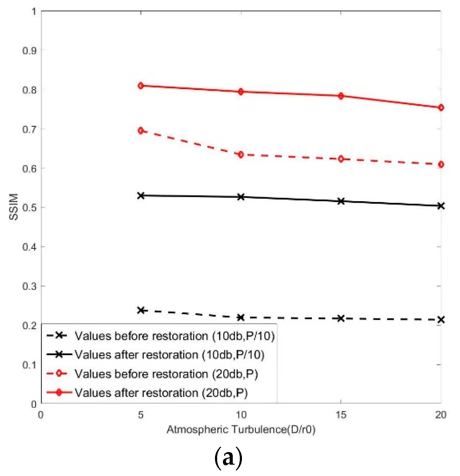
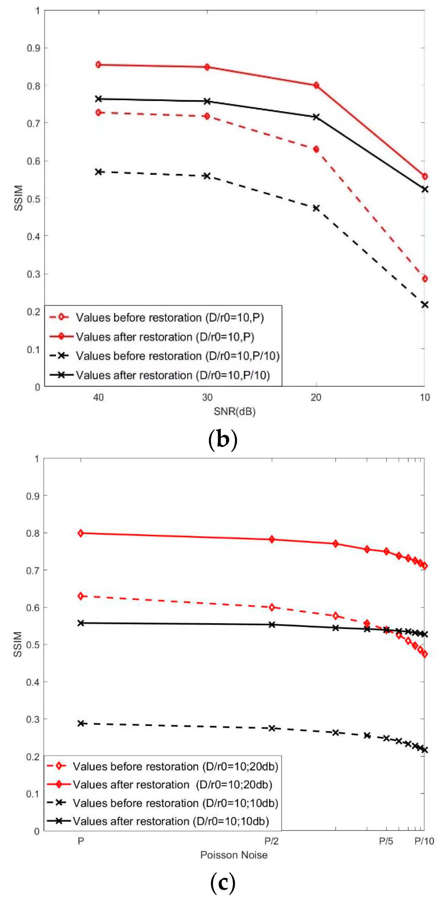
3.4. Quality Evaluation of Restored Image

In this section, structural similarity (SSIM) is introduced to quantitatively evaluate the quality of images before and after restoration. The SSIM is defined as follows:

$$SSIM \left(Y_m,{\widehat{Y}}_m\right)=\frac{\left(2{\mu }_{Y_m}{\mu }_{{\widehat{Y}}_m}+c_1\right)\left(2{\sigma }_{Y_m{\widehat{Y}}_m}+c_2\right)}{\left({\mu }_{Y_m}^2+{\mu }_{{\widehat{Y}}_m}^2+c_1\right)\left({\sigma }_{Y_m}^2+{\sigma }_{{\widehat{Y}}_m}^2+c_2\right)}$$

(12)

where $Y_m$ represents the image before or after restoration, and ${\widehat{Y}}_m$ represents the diffraction-limited image. ${\mu }_{Y_m}$ and ${\sigma }_{Y_m}^2$ denote the mean value and the variance of $Y_m$, respectively. So do ${\mu }_{{\widehat{Y}}_m}$, ${\sigma }_{{\widehat{Y}}_m}^2$ and ${\widehat{Y}}_m$.${\sigma }_{Y_m{\widehat{Y}}_m}$ is the covariance of $Y_m$ and ${\widehat{Y}}_m$. $c_1$ and $c_2$ are the constant terms used to avoid system errors caused by denominator 0. After restoration, the larger the SSIM, the higher the restored image quality, and the more effective the image restoration algorithm.

SSIM curves before and after restoration for the satellite image are given in Figure 4, where Figure 4a shows SSIM vs. atmosphere turbulence levels with constant SNR and Poisson noise, Figure 4b presents SSIM vs. SNRs with constant turbulent strength and Poisson noise, and relationship between SSIM and Poisson noise is given in Figure 4c with constant turbulent strength and SNR.

Figure 4. Curves of SSIM under different atmospheric turbulence and mixed noise: (a) SSIM vs. atmosphere turbulence levels with constant SNR and Poisson noise; (b) SSIM vs. SNRs with constant turbulent strength and Poisson noise; (c) SSIM vs. Poisson noise with constant turbulent strength and SNR.

Between SSIM and Poisson noise is given in Figure 4c with constant turbulent strength and SNR.

From Figure 4a, one can see that the change in turbulence strength has little effect on the SSIM whether the mixed noise is large (10 dB, P/10) or small (20 dB, P). When the mixed noise is 10 dB and P/10, the SSIM can reach 0.5 after restoration. Compared with the initial SSIM (0.2), the restored images’ quality is significantly improved. When the mixed noise is 20 dB and P (D/r₀ = 10), the SSIM ranges from 0.63 (before restoration) to 0.79 (after restoration).

As shown in Figure 4b, the SSIM ranges from 0.72 and 0.85 when SNR is 30 dB (D/r₀ = 10, P) and when D/r₀, P keep unchanged, and SNR is 10 dB, the corresponding SSIM is from 0.29 to 0.56. Compared with those before restoration, SSIMs are significantly improved, and the smaller the SNR, the more significant the improvement of SSIMs.

Figure 4c illustrates SSIM vs. Poisson noise with constant turbulent strength and SNR. When Poisson noise is P (D/r₀ = 10, SNR = 10 dB), SSIMs before and after image restoration are 0.29 and 0.56, respectively. The corresponding SSIMs are 0.21 and 0.53, respectively, when the Poisson noise is P/10 (D/r₀ = 10, SNR = 10 dB). The above data show that SSIMs after image restoration are improved obviously, and the greater the Poisson noise intensity, the greater the improvement of the image.

Based on the above-mentioned results from Figure 4, one can obtain that the six-channel MCAM algorithm proposed in this paper has a good restoration performance on blurred images degraded by atmospheric turbulence and mixed noise.

3.5. Effect of Image Restoration

In this section, we test the performance of the proposed method and compare it with the derivative-based alternate direction optimization method (D-ADMM) [24]. D-ADMM also adopts the alternating minimization algorithm without MC.

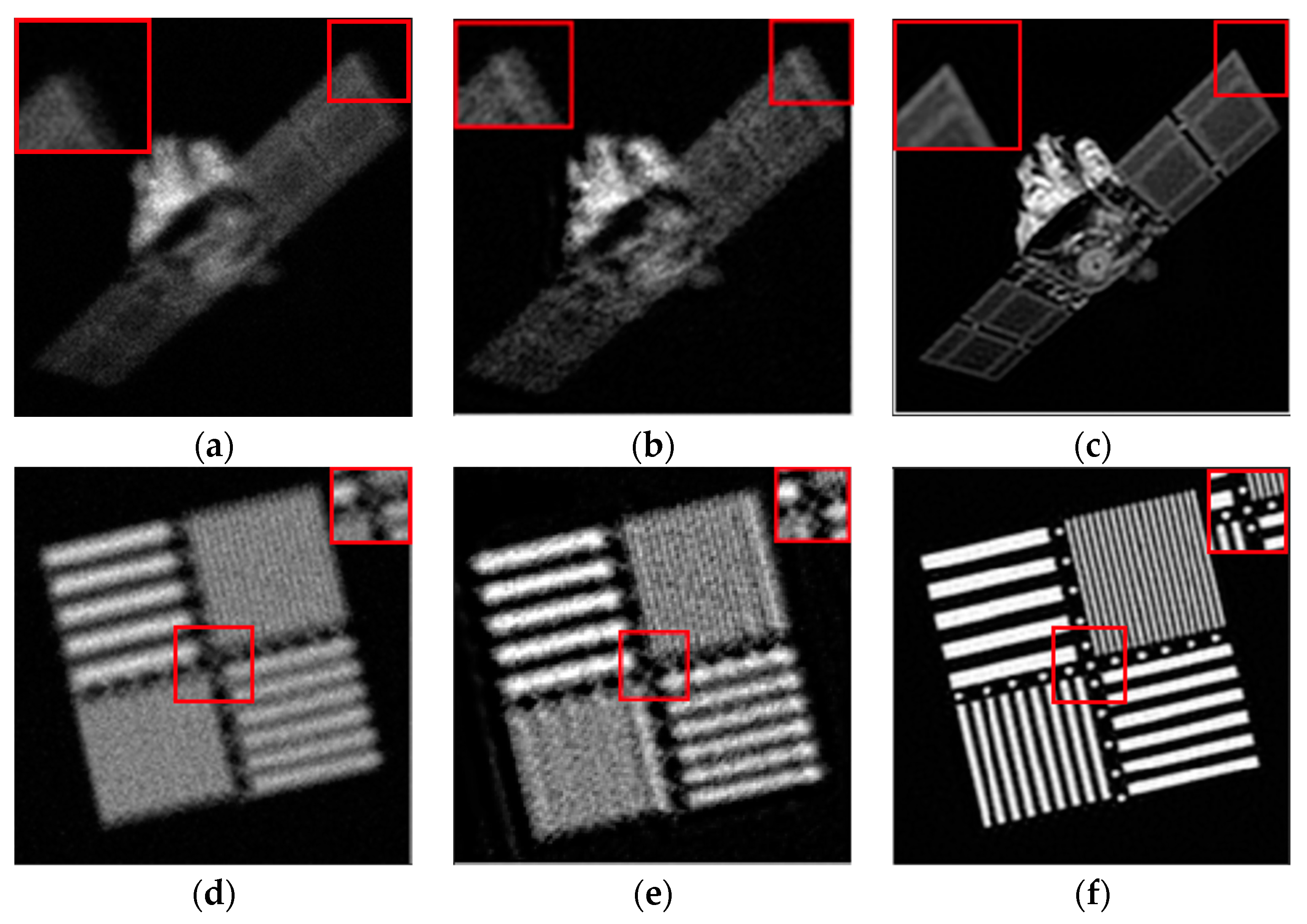
3.5.1. Restoration Results under the Condition of Moderate Turbulence and Mixed Noise

Figure 5 shows the degraded and restored images of satellites and streaks under the condition of moderate turbulence (D/r₀ = 10) and mixed noise (SNR = 20 dB, P), where (a,d) are two random degraded images, (b,e) are restored images by D-ADMM, (c,f) are restored results by our MCAM.

Figure 5. Reconstruction results of objects imaging degraded by moderate turbulence (D/r₀ = 10) and mixed noise (SNR = 20 dB, P). (a,d) are random degraded images, (b,e) are recovery images by D-ADMM, and (c,f) are reconstruction results by MCAM.

It can be seen from Figure 5a,d that the degraded images of satellites and streaks have blurred details, but the structural features of the object are relatively recognizable. When D-ADMM is used, some details of the degraded images are optimized while the restored images (Figure 5b,e) are still indistinct. From Figure 5c,f, one can see that the proposed method successfully removes the blurry details and the overall structure is basically consistent with the diffraction-limited image.

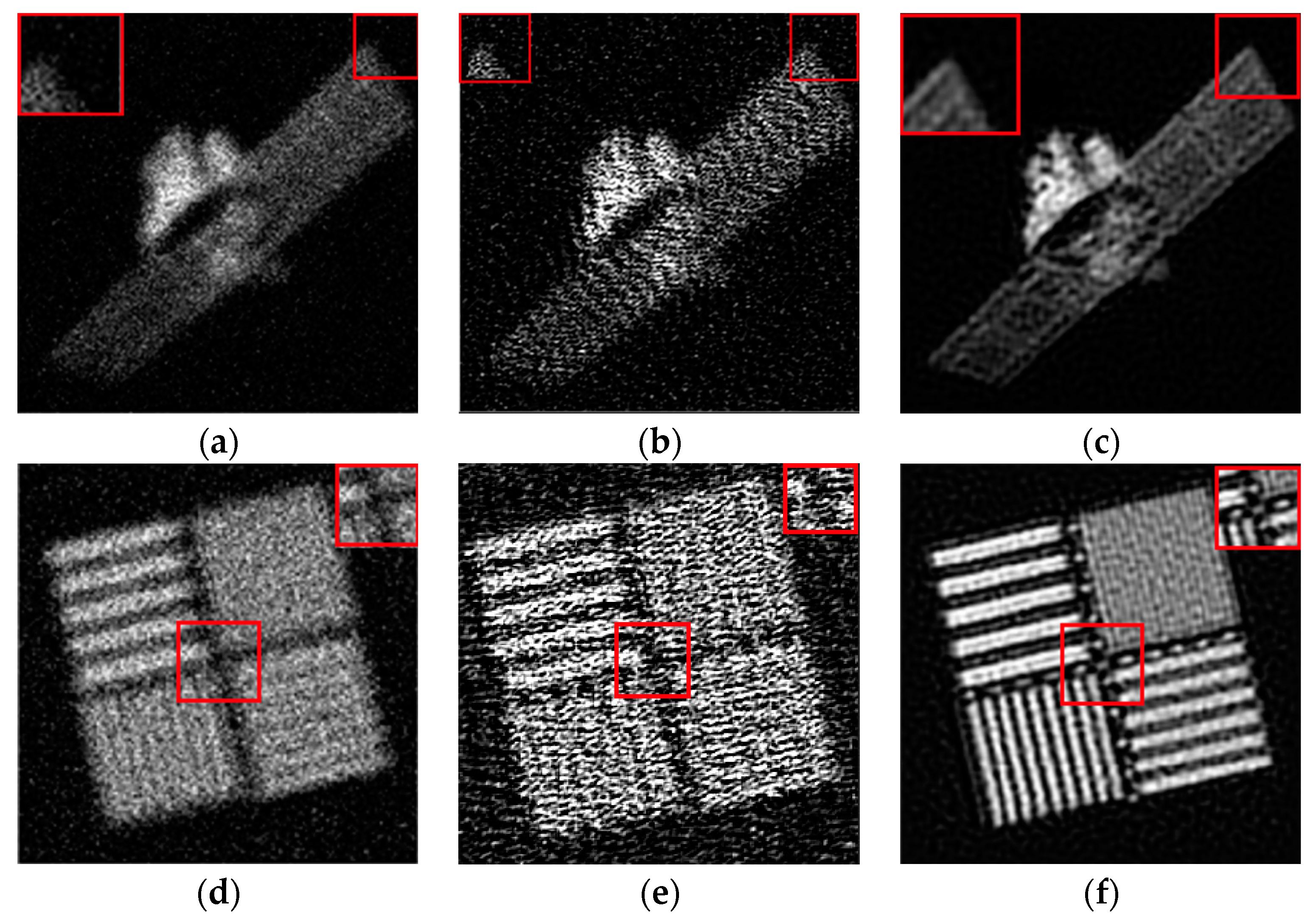
3.5.2. Restoration Results under the Influence of Strong Turbulence and Mixed Noise

The degraded and restored images of satellites and streaks under the condition of strong turbulence (D/r₀ = 20) and mixed noise (SNR = 10 dB; P/10) are presented in Figure 6, where (a,d) are degraded images, (b,e) are restored images by D-ADMM and (c,f) are restored results by MCAM. Different from the case of moderate turbulence, the degraded images are severely distorted in the case of strong turbulence. Restored images by D-ADMM are not ideal while restored images by MCAM take on a satisfying visual effect.

Figure 6. Reconstruction results of objects imaging degraded by strong turbulence (D/r₀ = 10) and mixed noise (SNR = 20 dB, P). (a,d) are random degraded images, (b,e) are recovery images by D-ADMM, and (c,f) are reconstruction results by MCAM.

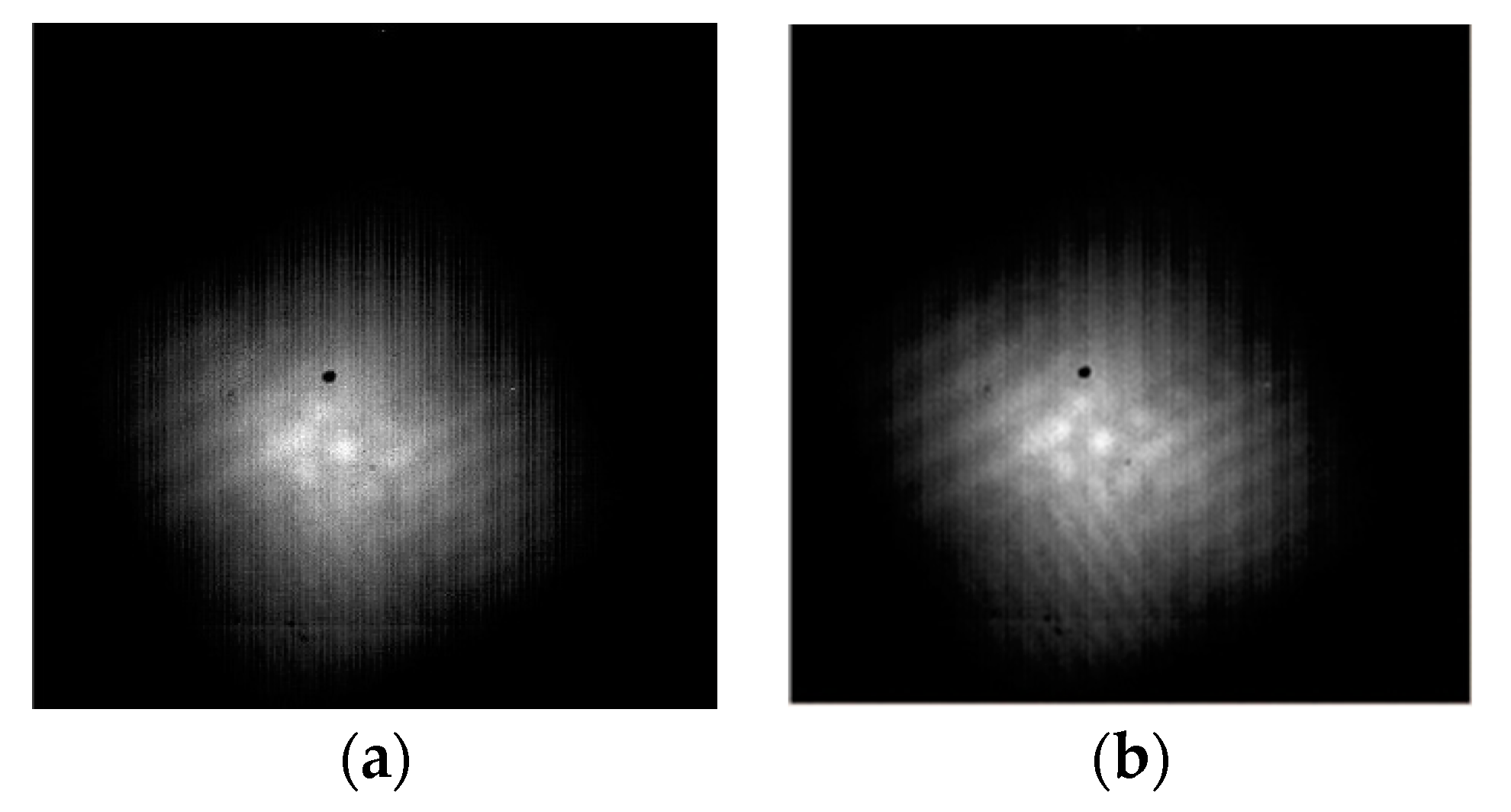
3.5.3. Restoration Results by Actual Experiment

As seen from the above discussion, MCAM can efficiently recover the images suffered from atmospheric turbulence and mixed noise by simulation. To test and verify the algorithm’s performance, an actual experiment is executed under the condition of horizontal atmosphere. A piece of stripe board was set as a space object and placed 2.4 km away from the observation telescope with an aperture of 1.3 m. We obtained two hundred pictures captured by CCD. Figure 7a–c shows three blurred images selected randomly from some group with six pictures. Figure 7d is the final reconstructed image by six-channel alternating minimization. By visual observation, one can see that the definition and the structural features of the object in Figure 7d are far better than Figure 7a–c. Thus, it can be seen that the actual experiment also fully validates the MCAM has strong stability and adaptability.

Figure 7. (a–c) Are randomly three blurred pictures, and (d) is the reconstructed image by MCAM.

4. Conclusions

In order to remove the impact of atmospheric turbulence and mixed noise on the imaging quality of astronomical or space objects, we propose a multi-channel alternating minimization method based on the theory of blind deconvolution MCAM. The performance of the approach is discussed from three aspects: the number of channels, the convergence speed, and the image restoration effect.

From the relationship between MSE and the number of frames, we can see that six channels are the optimal number of channels for processing degraded images. NRMSE curves show MCAM can converge quickly after two iterations. Quantitative analysis based on the SSIM verifies that the greater the influence of turbulence and the stronger the mixing noise, the higher the quality of restored images. Image reconstruction results prove the effectiveness of the method proposed in this paper. Compared with the previous image restoration methods limited to single-channel or weak turbulence, MCAM has strong robustness to strong turbulence levels and mixed noise. The above results can provide a reference for the restoration of degraded images by atmospheric turbulence and mixed noise. Future work involves extending this approach to moving objects with variant blur.

References

- Yong, J.; Tian, Y.; Xu, K.; Rao, C. An adaptive optics system control method combined with image restoration technology. Acta Phys. Sin. 2020, 69, 253–262. [Google Scholar] [CrossRef]
- Wang, K. Research on Adaptive Optics Correction Technology for Atmospheric Turbulent Wavefront Distortion; University of Chinese Academy of Sciences: Beijing, China, 2021; p. 000044. [Google Scholar]
- Ren, D.Q.; Zhang, T.Y.; Wang, G. A low-cost and high-performance technique for adaptive optics static wavefront correction. Res. Astron. Astrophys. 2021, 21, 263–270. [Google Scholar] [CrossRef]
- Banham, M.R.; Katsaggelos, A.K. Digital image restoration. IEEE Signal Process. Mag. 1997, 14, 24–41. [Google Scholar] [CrossRef]
- Fang, L.J.; Zuo, H.Y.; Pang, L.; Yang, Z.; Zhang, X.; Zhu, J. Image reconstruction through thin scattering media by simulated annealing algorithm. Opt. Lasers Eng. 2018, 106, 105–110. [Google Scholar] [CrossRef]
- Yang, H.Y.; Su, X.Q.; Chen, S.M. Blind Image Deconvolution Algorithm Based on Sparse Optimization with an Adaptive Blur Kernel Estimation. Appl. Sci. 2020, 10, 2437. [Google Scholar] [CrossRef]
- Xie, X.; Liu, Y.; Liang, H.; Zhou, J. Speckle correlation imaging: From point spread function to all elements of light field. J. Opt. 2020, 40, 71–82. [Google Scholar]
- Wang, J.L.; Li, B.H.; Zhang, X.L. A novel hybrid algorithm for lucky imaging. Res. Astron. Astrophys. 2021, 21, 156–168. [Google Scholar] [CrossRef]
- Xiang, M.; Pan, A.; Liu, J.P.; Xi, T.; Guo, X.; Liu, F.; Shao, X. Phase Diversity-Based Fourier Ptychography for Varying Aberration Correction. Front. Phys. 2022, 10, 848943. [Google Scholar] [CrossRef]
- Andrews, H.C.; Hunt, B.R. Digital Image Restoration. Pattern Recognit. 1979, 11, 75. [Google Scholar]
- Ayers, G.R.; Dainty, J.C. Iterative blind deconvolution method and its applications. Opt. Lett. 1988, 13, 547–549. [Google Scholar] [CrossRef]
- Molina, R.; Mateos, J.; Katsaggelos, A.K. Blind deconvolution using a variational approach to parameter, image, and blur estimation. IEEE Trans. Image Process. 2006, 15, 3715–3727. [Google Scholar] [CrossRef] [PubMed]
- Schulz, T.J. Multiframe blind deconvolution of astronomical images. J. Opt. Soc. Am. A 1993, 10, 1064–1073. [Google Scholar] [CrossRef]
- Kenig, T.; Kam, Z.; Feuer, A. Blind image deconvolution using machine learning for three-dimensional microscopy. IEEE Trans. Pattern Anal. Mach. Intell. 2010, 32, 2191–2204. [Google Scholar] [CrossRef] [PubMed]
- Li, X.; Wu, Y.; Fang, Z.; Xu, Q.; Yang, H.; Yang, H. Post-processing of adaptive optics images based on multi-channel blind recognition. Acta Photon. Sin. 2020, 49, 0201003. [Google Scholar]
- Sroubek, F.; Milanfar, P. Robust multichannel blind deconvolution via fast alternating minimization. IEEE Trans. Image Process. 2011, 21, 1687–1700. [Google Scholar] [CrossRef]
- Yang, H.; Li, S.; Li, X.; Zhang, Z.; Yang, H.; Liu, J. Blind restoration of turbulence degraded images based on two-channel alternating minimization algorithm. Optoelectron. Lett. 2022, 18, 122–128. [Google Scholar] [CrossRef]
- Chen, L. Several Types of Methods for Solving Constrained Optimization Problems Based on Augmented Lagrangian Functions; Hunan University: Changsha, China, 2016; pp. 5–24. [Google Scholar]
- Wang, X. Laplacian operator-based edge detectors. IEEE Trans. Pattern Anal. Mach. Intell. 2007, 29, 886–890. [Google Scholar] [CrossRef]
- Roddier, N.A. Atmospheric wavefront simulation using Zernike polynomials. Opt. Eng. 1990, 29, 1174–1180. [Google Scholar] [CrossRef]
- Yang, H.; Li, X. The influence of imaging system noise on the correction effect of adaptive optics without wavefront detection. China Laser 2010, 37, 2520–2525. [Google Scholar] [CrossRef]
- Zhang, Z. Research on Poisson ImageDenoising and Deblurring Based on Variation Model; Nanjing University of Science and Technology: Nanjing, China, 2015; pp. 51–68. [Google Scholar]
- Chowdhury, M.R.; Qin, J.; Lou, Y. Non-blind and blind deconvolution under poisson noise using fractional-order total variation. J. Math. Imaging Vis. 2020, 62, 1238–1255. [Google Scholar] [CrossRef]
- Ren, D.W.; Zhang, H.Z.; Zhang, D.; Zuo, W. Fast total-variation based image restoration based on derivative alternated direction optimization methods. Neurocomputing 2015, 170, 201–212. [Google Scholar] [CrossRef]
Publisher’s Note: MDPI stays neutral with regard to jurisdictional claims in published maps and institutional affiliations. |
© 2022 by the authors. Licensee MDPI, Basel, Switzerland. This article is an open access article distributed under the terms and conditions of the Creative Commons Attribution (CC BY) license (https://creativecommons.org/licenses/by/4.0/).