Equivalent Current Systems of Quiet Ionosphere during the 24th Solar Cycle Derived from the Geomagnetic Records in China

Abstract

External and internal equivalent current systems of solar quiet (Sq) were obtained using the spherical harmonic analysis (SHA) method with a “mirror” technique based on geomagnetic records from 46 stations in China during 2008–2019. It is the first attempt to investigate Sq currents using so many stations in the China region for a long period. On the basis of criterion Kp ≤ 2+, geomagnetic vector data were selected to represent monthly Sq variations. After calculating the equivalent currents for each month and each Lloyd season, Sq variation was analyzed in relation to the solar cycle and season. The intensities of both external and internal Sq currents were found consistent with solar activity for the same month or season, while the positions of the current foci were evidently unaffected by solar activity. The intensities of Sq currents also exhibited primary semiannual (annual) variation in the periods of high (low) solar activity. The latitude of the internal current vortex showed evident seasonal variation in Lloyd seasons with high (low) values in the D (J) season, while the external current vortex exhibited no obvious seasonal variation. The strongest correlation between external and internal foci was found in D season, and the internal current foci usually appeared 20–40 min earlier than the external ones. Owing to the complex mechanisms behind Sq variation, some findings will need further analysis in the future.

1. Introduction

Daily variation of geomagnetic field is mainly caused by the current in the ionosphere, especially during the geomagnetic quiet time, i.e., the solar quiet (Sq) current [1,2]. The Sq current has a regular period of approximately 24 h [3]. It is principally generated by the ionospheric dynamo effect of diurnal and semidiurnal tidal winds applying a force on locally ionized particles in situ via solar heating in the presence of Earth’s main field [4,5,6,7,8,9,10,11,12,13]. Therefore, the Sq current primarily relates to the neutral tidal winds, conductivities in the dynamo region, and Earth’s main field [14]. Generally, the Sq current flows at an altitude of between 100 and 170 km in the ionosphere owing to the large Pedersen and Hall conductivities in this region [15]. In mid–low latitudes, the Sq current forms a current vortex located in each hemisphere on the sunlit side of the Earth [16]. The current vortex flows anticlockwise in the Northern Hemisphere and clockwise in the Southern Hemisphere [17]. The centers of the current vortices are at approximately 11:30 local time (LT) and ± 30° latitude [3].

Owing to the conductivity of Earth’s medium, the Sq current system in the ionosphere can induce a secondary current in Earth’s interior. Therefore, the Sq current flowing in the ionosphere is called the external source current, and the corresponding current induced in the interior is called the internal source current [3]. The internal part has a pattern similar to that of the external part, but the direction is reversed with a local time difference in phase [18]. Actually, the observed daily variation of the geomagnetic field during the quiet time is the superposition of the variation caused by both the external and internal Sq currents, whereby the internal one accounts for approximately one-third of the daily variation [19].

Using the spherical harmonic analysis (SHA) method, the external and internal parts of the geomagnetic field can be separated [20]. Schuster [21] first used SHA to analyze the daily variations of quiet. Then, Chapman and Bartels [22] developed a time-to-longitude conversion technique for SHA. The Sq current is assumed fixed in a position synchronized with the Sun and the daily record of an observatory on the ground obtains a 360° sample of the current. Many studies have used SHA to investigate Sq variation. One method of SHA involves global study of Sq using observatories distributed around the world [9,23,24,25,26]. Another approach uses observatories well distributed in latitude but limited in a longitudinal zone, thereby obtaining a “slice” of data [27]. If the data is along a meridian chain throughout the Northern Hemisphere and the Southern Hemisphere, the two vortices of Sq current can be obtained by SHA. Earlier representative studies of the Sq current used data of a meridian chain from the Circum-pan Pacific Magnetometer Network, which is known as the 210 Magnetic Meridian [16,28,29]. Utilizing a “mirror” technique, the slice data of one hemisphere can be appropriately modeled for the opposite hemisphere. Using this method with SHA, Campbell and Schiffmacher [12] compared Sq currents in four regions of the Northern Hemisphere: North America, Europe, central Asia, and eastern Asia. Additionally, data from 18 observatories were used to study the Sq current in the India–Siberia region [30]. Similarly, Campbell and Schiffmacher [31] used slice data from the Southern Hemisphere and the mirror technique to examine Sq currents in the South American, African, and Australian regions.

It is well known that the Sq current varies not only with a period of approximately 24 h, but also in terms of amplitude and phase depending on solar activity and season [17,32,33,34,35]. Using SHA, previous related studies investigated the effect of representatively quiet or active years in the solar cycle [24,36,37], while others examined Sq features by analyzing short-term (several years) data [15,27,29,30]. To investigate the long-term variation of Sq, some studies applied SHA to the data of global or meridian chain observatories during solar cycles [16,25,26].

Analysis of long-term geomagnetic data revealed that Sq currents have annual and semiannual variations [28]. The main characteristic of the annual variation is that current intensity in local summer is much greater than that in local winter. The characteristic of the semiannual variation is that current intensity maxima occur around the equinoxes. Some studies suggested that the semiannual variation of Sq is evident primarily in years of higher solar activity [26,31.37]. However, Stening [38] found that semiannual variation of Sq occurs even during the solar minimum period. Additionally, Sq exhibits distinct seasonal variation between the Northern Hemisphere and the Southern Hemisphere in periods of different solar activity [15,16]. Currently, comprehensive understanding of the physical processes behind Sq variation remains lacking.

The present study used data from the dense network of observation stations in China, together with the SHA method and the mirror technique pioneered by Campbell [12,30,31,39], to separate the external and internal equivalent currents of Sq in the China region, marking the long-term (2008–2019) investigation of Sq currents using so many stations in China for the first time. The objective was to extract the monthly, yearly and seasonal variation features of Sq based on long-term reliable ground observatory records and to examine their relationships with the solar cycle.

2. Materials and Methods

The data used in this study were acquired by the Geomagnetic Network of China (GNC) and INTERMAGNET. GNC completed the “China Digital Seismic Observation Network” project in 2007 [40]. With strict quality control of geomagnetic data, GNC can distribute observational data within 48 h [41,42]. Observations used in the present study included those from GNC 45 stations and those from the Beijing Ming Tombs (BMT) INTERMAGNET station located in Beijing. We used absolute magnetic field components with one-minute time resolution in North East Center (NEC) coordinates, in which X points to the North, Y points to the East and Z in the vertical direction points to the center of the Earth. The finer temporal resolution permitted better determination of the Sq phase [43]. Figure 1 shows the distribution of the stations used in this study. The number of observatories used for each month might have differed slightly depending on data availability and data quality. The Sq equivalent currents were calculated for the 12-year period 2008–2019 which covers the 24th solar cycle, indicated by the sunspot numbers as shown in Figure 2. The sunspot number data were derived using a running mean of the monthly sunspot numbers over a 13-month window centered on the corresponding month. This form of running mean has become the base standard for the conventional definition of times of minima and maxima in solar cycles

In this paper, geomagnetic quiet days (in local time) for each month are defined as days when all eight 3-h planetary geomagnetic disturbance index Kp values are ≤2+. Some earlier related studies also used this criterion [16,37,44]. The Kp index is provided by the World Data Center for Geomagnetism, Kyoto. After selecting the geomagnetic quiet days, the time series superposition method is used to average the geomagnetic data representing Sq variation for every station in each month. A quiet level baseline is defined as the mean of nighttime values for each day (i.e., minute values from 0000–0200 and from 2200–2359 LT). We compute ΔX, ΔY and ΔZ by subtracting the baseline value from X, Y, and Z absolute geomagnetic components. In this paper, for brevity, we use X, Y, and Z to represent the quiet variation of ΔX, ΔY, and ΔZ in each month.

The Sq variation is mainly composed of several harmonics with diminishing amplitudes [3]. Before conducting SHA, an important assumption is that the longitude and local time are equivalent [15,30]. Using the Fast Fourier Transform, the coefficients of cosine and sine can be obtained. In Equation (1), a(m) and b(m) indicate the coefficients of cosine and sine for each geomagnetic component respectively. Here, M represents the orders of the harmonic waves and λ is the longitude which is equivalent to the local time. Therefore, the observed value (S) representing each component can be calculated as the sum of the cosine and sine of λ in different orders:

$$\mathrm{S}={\displaystyle \sum }_{\mathrm{m}=0}^{\mathrm{M}}\left[\mathrm{a}\left(\mathrm{m}\right)\cos \mathrm{m}\mathsf{\lambda }+\mathrm{b}\left(\mathrm{m}\right)\sin \mathrm{m}\mathsf{\lambda }\right]$$

(1)

Taking station BMT as an example, Figure 3 shows the variation of the coefficients for the cosine and sine in different seasonal months of the solar activity year of 2014. The first four rows indicate the amplitude of a(m) and b(m) in March, June, September, and December 2014, respectively, and each column illustrates one geomagnetic component. It can be seen that the amplitude of the 8th and higher harmonic coefficients is much smaller and stable, i.e., generally approaching zero. The lower row of Figure 3 represents the synthetic variation of the first 8 harmonic waves (solid lines) and the mean value of Sq variation at BMT in different months (dashed line). It is evident that the synthetic variation of the first 8 harmonic waves nearly coincides with the mean value at the observatory. The error between the synthetic and the mean value is <10⁻¹⁵ nT. This indicates that the synthetic value is enough to represent the Sq variation of each month, and we set M as 8 in this study. Having obtained the Fourier coefficients for each station in China, we used the mirror technique pioneered by Campbell [12,30,31,39] to model the Fourier coefficients of the Southern Hemisphere from those of the Northern Hemisphere by assuming that the components of Y and Z are oppositely directed and shifted temporally by six months. The Fourier coefficients modeled in the opposite hemisphere are properly the boundary conditions for the analysis region, and the results of SHA are applicable only to the original region of the primary hemisphere [31].

In the spherical coordinate system, the scalar potential of the geomagnetic field satisfies the Laplace equation. The magnetic potential for quiet daily variations can be expanded by Schmidt’s function $P_n^m\left(\cos \mathrm{\theta }\right)$ in the latitudinal direction. We performed SHA for the orders of m = 0 − M and degrees n = m − (m + N), i.e., similar representation to Pedatella et al. [15] and Yamazaki et al. [16]. The geomagnetic components of Sq on the surface of Earth can be expressed by Equation (2):

$$\begin{gathered} \mathrm{X}={{\displaystyle \sum }}_{\mathrm{m}=0}^{\mathrm{M}}{{\displaystyle \sum }}_{\mathrm{n}=\mathrm{m}}^{\mathrm{m}+\mathrm{N}}\left({\mathrm{p}}_{\mathrm{n}}^{\mathrm{m}}\cos \mathrm{m}\mathsf{\lambda }+{\mathrm{q}}_{\mathrm{n}}^{\mathrm{m}}\sin \mathrm{m}\mathsf{\lambda }\right)\frac{\partial {\mathrm{P}}_{\mathrm{n}}^{\mathrm{m}}\left(\cos \mathsf{\theta }\right)}{\partial \mathsf{\theta }}, \\ \mathrm{Y}={{\displaystyle \sum }}_{\mathrm{m}=0}^{\mathrm{M}}{{\displaystyle \sum }}_{\mathrm{n}=\mathrm{m}}^{\mathrm{m}+\mathrm{N}}\left({\mathrm{p}}_{\mathrm{n}}^{\mathrm{m}}\sin \mathrm{m}\mathsf{\lambda }-{\mathrm{q}}_{\mathrm{n}}^{\mathrm{m}}\cos \mathrm{m}\mathsf{\lambda }\right)\frac{{\mathrm{mP}}_{\mathrm{n}}^{\mathrm{m}}\left(\cos \mathsf{\theta }\right)}{\sin \mathsf{\theta }}, \\ \mathrm{Z}={{\displaystyle \sum }}_{\mathrm{m}=0}^{\mathrm{M}}{{\displaystyle \sum }}_{\mathrm{n}=\mathrm{m}}^{\mathrm{m}+\mathrm{N}}\left({\mathrm{r}}_{\mathrm{n}}^{\mathrm{m}}\cos \mathrm{m}\mathsf{\lambda }+{\mathrm{s}}_{\mathrm{n}}^{\mathrm{m}}\sin \mathrm{m}\mathsf{\lambda }\right){\mathrm{P}}_{\mathrm{n}}^{\mathrm{m}}\left(\cos \mathsf{\theta }\right), \end{gathered}$$

(2)

where θ is the colatitude, and λ is the longitude equal to the local time. In comparison with Equation (1), the Fourier coefficients of a(m) and b(m) for each component can be calculated by ${\mathrm{p}}_{\mathrm{n}}^{\mathrm{m}}$ and ${\mathrm{q}}_{\mathrm{n}}^{\mathrm{m}}$ or ${\mathrm{r}}_{\mathrm{n}}^{\mathrm{m}}$ and ${\mathrm{s}}_{\mathrm{n}}^{\mathrm{m}}$ using Schmidt’s function to obtain the change of latitude direction. For example, Figure 4 exhibits the Fourier coefficients of m = 4 fitting by Schmidt’s function with N = 60 for the stations of China in March 2014. It can be seen that the Fourier coefficients of each station (red crosses) are well fitted by ${\mathrm{P}}_{\mathrm{n}}^{\mathrm{m}}\left(\cos \mathsf{\theta }\right)$ (the blue line). It is also evident that the dense distribution of stations between 15–50 °N is suitable for analyzing the variation of Sq.

To examine the proper value of N, error analysis was performed for March, June, September, and December 2014. As an example shown in Figure 4 for m = 4 and N = 60, we calculated the mean errors between the Fourier coefficients (red crosses) and Schmidt’s function (blue line) for all stations in each panel. Then, we summed the mean errors from m = 0−M (M = 8) corresponding to different N for each month. Figure 5 illustrates the sum of the mean errors for N = 10−100 with a step of 10. It can be seen that when N =10, the sum of the errors is >5 nT for each of the four different months. As the value of N increases, the sum of the errors decreases substantially, dropping by approximately 0.27–0.95 nT for the different months from values of N = 10−60. However, from N = 60−100, the sum of the errors increases by only 0.01 nT. This means that for N > 60, the improvement of the Schmidt’s function fitting error is much limited. Therefore, in the present study, the value of N = 60 was taken as the maximum reasonable value.

The distribution of observation stations in China is dense but inhomogeneous. Therefore, it should be considered whether the stations used in the present study can represent Sq variation in China. We performed an experiment based on observatory data acquired in March, June, September, and December 2014. All stations used in the comparison were omitted from the calculation of the coefficients of Schmidt’s function. Then, error analysis was undertaken between the model result (coefficient multiplying the Schmidt’s function) and the comparison station. The error was calculated from the average difference between the model result and the observatory data of Sq variation throughout the entire day (1440 data) for each month. Following comparison of approximately 40 stations, the error contours of the quiet days in each month are illustrated in Figure 6. Each row in the figure represents a different month (i.e., March, June, September, and December 2014), and each column represents the geomagnetic component of Sq. The black dots in the figure indicate the positions of the stations. It can be seen that the maximum error in the location of a station is approximately 5 nT for the X and Y components and approximately 2 nT for the Z component.

Table 1. Mean error (me) and root mean square (rms) of error for all the stations. (Unit: nT).

2014	Mar.		Jun.		Sep.		Dec.
	me	rms	me	rms	me	rms	me	rms
X	3.24	3.29	2.49	2.57	3.34	3.37	2.93	2.99
Y	3.17	3.25	3.42	3.51	1.91	2.07	2.30	2.34
Z	0.66	0.73	1.00	1.31	0.83	0.96	0.61	0.70

shows details of the mean error and root mean square of error for all the stations corresponding to the four months of interest in 2014. The analysis proves that the distribution of stations in China is sufficient to analyze the Sq variation.

Having obtained the coefficients of Schmidt’s function ${\mathrm{p}}_{\mathrm{n}}^{\mathrm{m}}$, ${\mathrm{q}}_{\mathrm{n}}^{\mathrm{m}}$, ${\mathrm{r}}_{\mathrm{n}}^{\mathrm{m}}$, and ${\mathrm{s}}_{\mathrm{n}}^{\mathrm{m}}$ based on all the stations in China, the Gauss coefficients are calculated using Equation (3):

$$\begin{gathered} {\mathrm{p}}_{\mathrm{n}}^{\mathrm{m}}={\mathrm{g}}_{\mathrm{n}}^{\mathrm{m}}+{\mathrm{j}}_{\mathrm{n}}^{\mathrm{m}}, \\ {\mathrm{q}}_{\mathrm{n}}^{\mathrm{m}}={\mathrm{h}}_{\mathrm{n}}^{\mathrm{m}}+{\mathrm{k}}_{\mathrm{n}}^{\mathrm{m}}, \\ {\mathrm{r}}_{\mathrm{n}}^{\mathrm{m}}={\mathrm{nj}}_{\mathrm{n}}^{\mathrm{m}}-\left(\mathrm{n}+1\right){\mathrm{g}}_{\mathrm{n}}^{\mathrm{m}}, \\ {\mathrm{s}}_{\mathrm{n}}^{\mathrm{m}}={\mathrm{nk}}_{\mathrm{n}}^{\mathrm{m}}-\left(\mathrm{n}+1\right){\mathrm{h}}_{\mathrm{n}}^{\mathrm{m}}. \end{gathered}$$

(3)

The Gauss coefficients ${\mathrm{j}}_{\mathrm{n}}^{\mathrm{m}}$ and ${\mathrm{k}}_{\mathrm{n}}^{\mathrm{m}}$ are for the external contributions, and ${\mathrm{g}}_{\mathrm{n}}^{\mathrm{m}}$ and ${\mathrm{h}}_{\mathrm{n}}^{\mathrm{m}}$ are for the internal contributions. Then, the external equivalent current ${\mathrm{J}}^{\mathrm{e}}$ and the internal equivalent current ${\mathrm{J}}^{\mathrm{i}}$ are obtained using Equation (4):

$$\begin{gathered} {\mathrm{J}}^{\mathrm{e}}=\mathrm{R}{{\displaystyle \sum }}_{\mathrm{m}=0}^{\mathrm{M}}{{\displaystyle \sum }}_{\mathrm{n}=\mathrm{m}}^{\mathrm{m}+\mathrm{N}}-\frac{1}{{\mathsf{\mu }}_0}\frac{2\mathrm{n}+1}{\mathrm{n}+1}\left[{\left(\frac{\mathrm{r}}{\mathrm{R}}\right)}^{\mathrm{n}}\left({\mathrm{j}}_{\mathrm{n}}^{\mathrm{m}}\cos \mathrm{m}\mathsf{\lambda }+{\mathrm{k}}_{\mathrm{n}}^{\mathrm{m}}\sin \mathrm{m}\mathsf{\lambda }\right){\mathrm{P}}_{\mathrm{n}}^{\mathrm{m}}\left(\cos \mathsf{\theta }\right)\right], \\ {\mathrm{J}}^{\mathrm{i}}=\mathrm{R}{{\displaystyle \sum }}_{\mathrm{m}=0}^{\mathrm{M}}{{\displaystyle \sum }}_{\mathrm{n}=\mathrm{m}}^{\mathrm{m}+\mathrm{N}}\frac{1}{{\mathsf{\mu }}_0}\frac{2\mathrm{n}+1}{\mathrm{n}}\left[{\left(\frac{\mathrm{R}}{\mathrm{r}}\right)}^{\mathrm{n}+1}\left({\mathrm{g}}_{\mathrm{n}}^{\mathrm{m}}\cos \mathrm{m}\mathsf{\lambda }+{\mathrm{h}}_{\mathrm{n}}^{\mathrm{m}}\sin \mathrm{m}\mathsf{\lambda }\right){\mathrm{P}}_{\mathrm{n}}^{\mathrm{m}}\left(\cos \mathsf{\theta }\right)\right], \end{gathered}$$

(4)

where r denotes the geocentric distance, ${\mathsf{\mu }}_0$ is the magnetic permeability of free space, and R is Earth’s radius (=6371 km). The external equivalent current of Sq flows in the ionospheric E layer, which is often termed the dynamo region owing to the large Pedersen and Hall conductivities [15]. The typical altitude of this region is generally 110 km [45]. Here, we take r = R + 110 km to evaluate the equivalent ionospheric Sq current, and r = R is used in calculating the internal equivalent current. As per the discussion in this section, the upper limits of the series truncation for order M and degree N are 8 and 60, respectively. We take 0.5° × 0.5° grids latitudinally and longitudinally (equivalent to 2 min local time) for SHA to study the external and internal equivalent currents of Sq.

3. Results

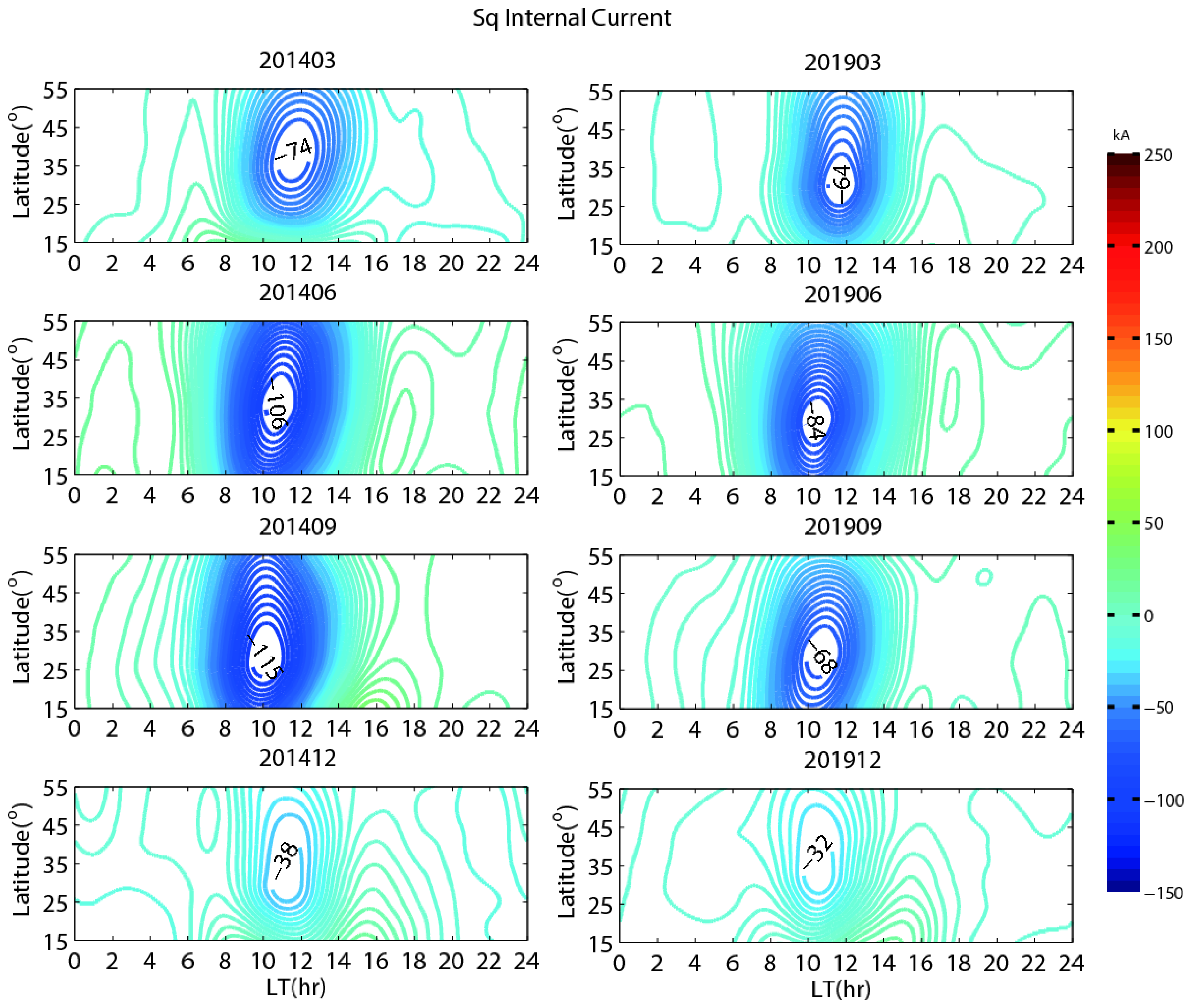
3.1. Sq Currents in Solar Maximum and Minimum Years

The SHA method with a mirror technique was applied to separate the external and internal equivalent currents of Sq in China. Using the sunspot number, as shown in Figure 2, we selected two years with a different level of solar activity. The solar maximum year 2014 and solar minimum year 2019 correspond to annual mean sunspot numbers of 113.6 and 3.6 respectively. For both years, the representative months of March, June, September, and December are used to compare the Sq currents. Each panel in Figure 7 shows the LT-Latitude distribution contour map of the external Sq current system in these two years. Positive contour lines indicate an anticlockwise direction of current flow. Each column illustrates the results for different months in one year. It is notable that the shape of the external Sq current is characterized by a dayside vortex in the Northern Hemisphere, consistent with the previous studies [16,22]. For the same month, it is evident that the external current intensity is much larger in the solar maximum year than that in the solar minimum year. The difference between the external current intensity in the same month of these two years ranges from 31 kA (March and June) to 76 kA (September). Another obvious observation is that the largest external current intensity out of the four months is in September for the solar maximum year 2014. However, it is in June for the solar minimum year 2019.

Figure 8 provides comparisons of the internal equivalent currents for these two years. The description of the figure is same as Figure 7. Different from the external current, negative contour lines indicate a clockwise direction of current flow, as an induced current from the external equivalent current. Similar to the external equivalent current, for the same month, the largest difference in internal current intensity appears in September (approximately 47 kA), but in December, the intensities of the internal currents for these two years are less different. The largest internal current intensity of the four months appears in September for the solar maximum year (2014). From Figure 7 and Figure 8, it can be determined that the intensities of the internal current are approximately half those of the external equivalent current at most times in both the solar maximum and the solar minimum years. However, in December 2014, the intensity of the internal current is approximately one third that of the external equivalent current. This might indicate that the intensity of the internal current relates not only to the external current, but also to the complex regional conductivity structure underground.

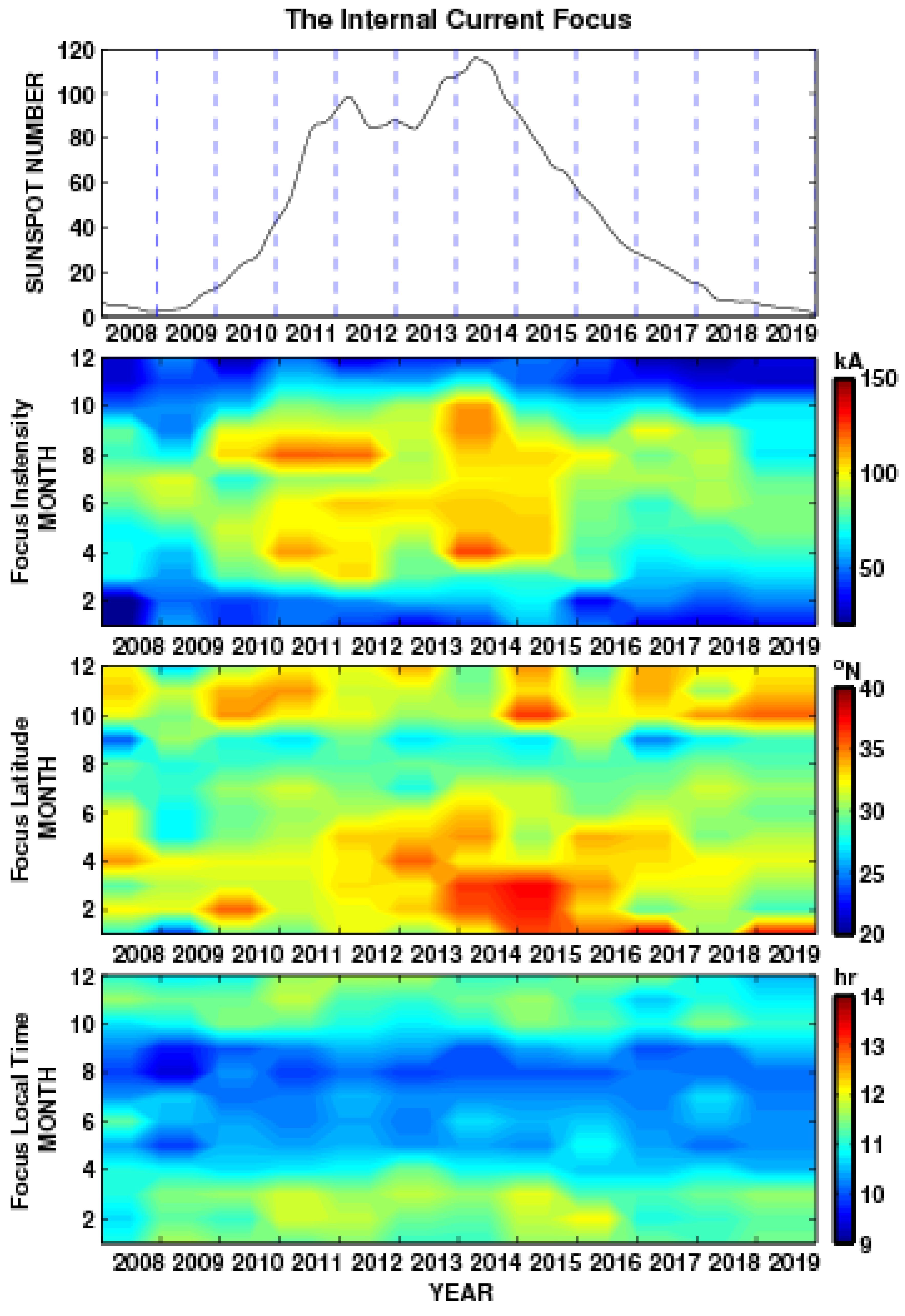
3.2. Variation of Sq Currents in the Solar Cycle

After calculating the external and internal equivalent currents of Sq in China for each month, we analyze the current vortex during the 12 years of interest. Three parameters such as vortex foci local time, latitude and intensity are investigated for the external and internal equivalent currents for each month.

Figure 9 and Figure 10 show the three parameters of current vortex foci for external and internal equivalent currents, respectively. In each figure, the top panel indicates the variation of monthly sunspot numbers during 2008–2019. The second to fourth panels depict contour maps of three parameters for the current vortex foci in the YEAR–MONTH diagram. The absolute value is used to represent the intensity of the internal equivalent current (hereafter, as the same). For both external and internal currents, the intensity in the same month is larger in years with higher solar activity than in other years, as evident during 2011–2014. The greatest intensity of the external current appears in April 2014, corresponding to approximately 238 kA. The greatest intensity of the internal current also appears in April 2014, corresponding to approximately 124 kA. The greatest intensities for both currents occur in the solar maximum year. This is consistent with the statement that the intensities of the external and internal equivalent current vortices are clearly controlled by changes in solar activity [16].

The most interesting feature in the month-to-month variations of current foci intensity is the existence of semiannual variation during years with higher solar activity. During 2011–2014, the intensity of the external current vortex has two extreme values: one around August–October, and the other around March–May (second panel in Figure 9). However, in June or July, the intensity of the external current vortex is lower than that in adjacent months at most times during 2011–2014. It is especially notable that the intensity in April 2014 for both external and internal current vortices is the maximum during the 12-year period. In the period of lower solar activity, the intensity of the external current vortex presents a pattern of annual variation with an extreme value around May–July (e.g., in 2009, 2018, and 2019 in the second panel of Figure 9). The intensity of the internal current vortex presents a pattern similar to that of the external current vortex, but it is even more evident (second panel in Figure 10). This finding is identical to the results of earlier studies [15,26,31,37].

There is little evident seasonal variation in the latitude of the external current vortex (third panel of Figure 9). The range of latitude changes from 24 °N to 36.5 °N. During the 12 years, the latitude of the external current vortex appears to reach to a low value in September, i.e., approximately 24.5–27 °N. However, there appears to be seasonal variation in the latitude of the internal current vortex, as shown in the third panel of Figure 10. The high value of the internal vortex latitude usually appears during January–March and October–December, with the value above 30 °N at most times and peaking at 38 °N. It indicates that the latitude of the internal current vortex in autumn and winter is higher than that in spring and summer.

The local time of both the external and the internal current vortices has significant seasonal variation in each year (as shown in the fourth panel of Figure 9 and Figure 10). The vortex foci appear in the prenoon sector during March–September and at around noon and in the afternoon sector during October–December and January–March. However, the local time of the external and internal current vortices does not show synchronous activity. For each month, the local time of the internal current vortex usually appears earlier than that of the external current vortex. During the 12-year period, the local time of the external (internal) vortex is in the range of 1018–1242 LT (0924–1206 LT).

To examine the relation between the current vortices and solar activity, we analyze the yearly means of sunspot numbers and three parameters of the external and internal current vortex foci. In Figure 11, the top panel shows the time sequence of the yearly means of sunspot numbers during the 12-year period. The subsequent six panels show the yearly means of the intensity, latitude, and local time of the external and internal current vortex foci. In the upper-right corner of each panel, the correlation coefficient between the sunspot numbers and the parameter of the vortex foci is presented. The dependence of the external and internal current intensities on solar activity is evident in this figure. The correlation coefficients of the external and internal current intensities with sunspot numbers are all >0.94, which probably reflects the solar-activity dependence of ionospheric conductivity [16]. The correlations between the latitude of the current vortex foci and the sunspots are relatively low, with coefficients of 0.403 and 0.489 for the external and internal foci, respectively. For the local time of the current vortex foci, the correlation coefficients with sunspots are better than those with latitude, but the values are still only 0.746 and 0.655 for the external and internal currents, respectively. This result agrees with the finding that changes in solar activity have little effect on the latitudinal and local-time position of Sq current foci [16].

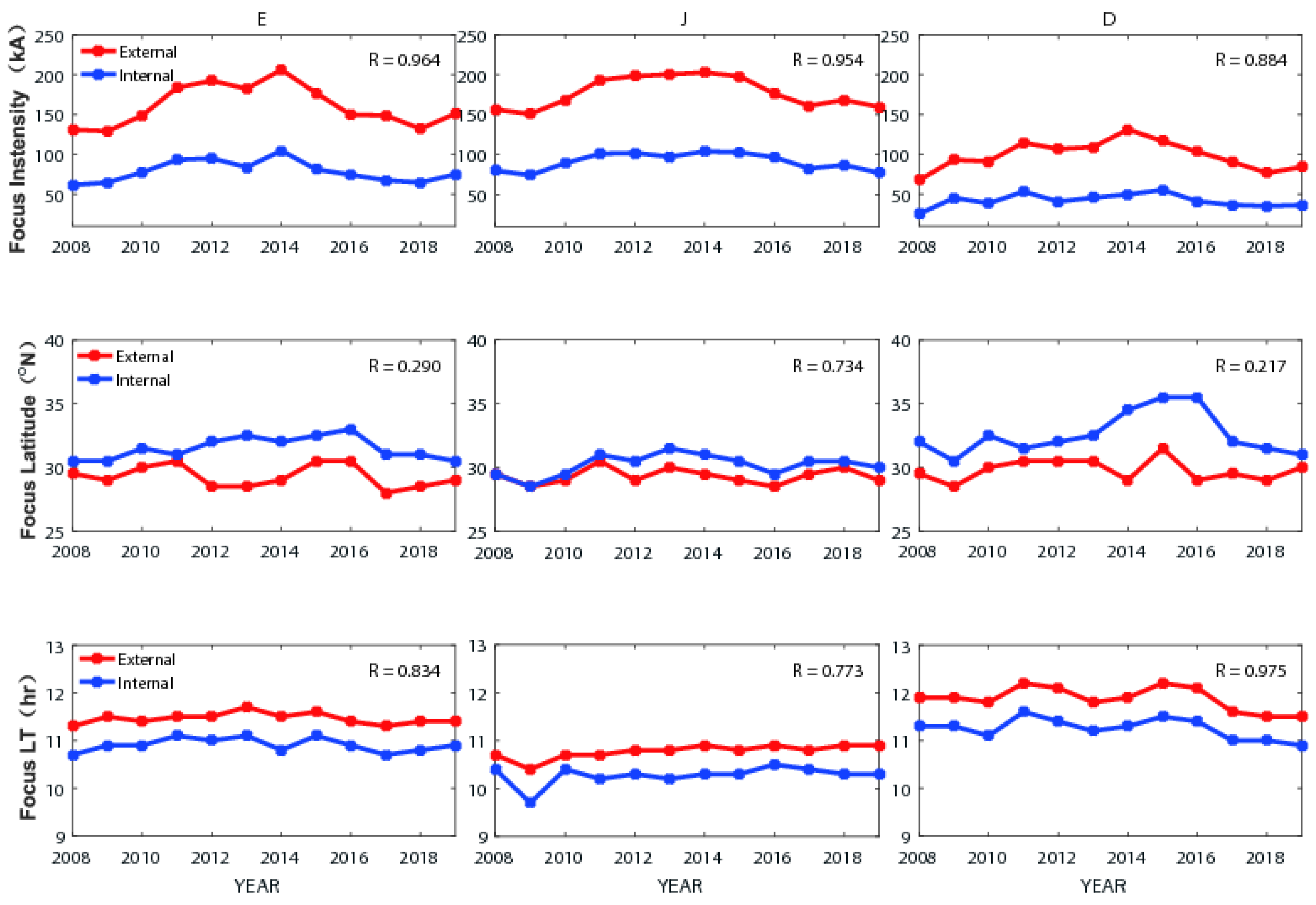
3.3. Variations of Sq currents in Lloyd seasons

Lloyd seasons are generally used in geomagnetism to analyze the seasonal variations of Sq. For Lloyd seasons, a year is divided into three seasons, i.e., the equinox E season (including March, April, September, and October), summer J season (including May, June, July, and August) and winter D season (including January, February, November, and December) [3,26,29]. Based on the Sq variation in each month described in the Section 3.2, we calculate the Sq variations in the Lloyd seasons using the average of the corresponding four-monthly geomagnetic values for every season. Similar to applying the SHA method with a mirror technique to the monthly Sq variations, the external and internal current systems in China for each Lloyd season are derived. The mirror part of the E season is also the E season, but the mirror part of the J (D) season is the D (J) season for the Southern Hemisphere. For all the mirror parts, the components of Y and Z are oppositely directed and are used as boundary conditions in the SHA method. We considered the Sq equivalent currents in the Northern Hemisphere in each season to represent the Sq variations in China during 2008–2019.

Figure 12, Figure 13 and Figure 14 show LT–Latitude contour maps of the flow of external and internal Sq currents in the Lloyd E, J, and D seasons, respectively, during the 12-year period. In each figure, each panel indicates the result for one year. The top four rows represent the external Sq currents and the bottom four rows represent the internal Sq currents. It is notable that the intensity of the external vortex in all the three seasons has a maximum value in the year with highest solar activity (2014), i.e., values of 206, 202, and 131, kA in the E, J, and D seasons, respectively. The minimum intensity of the external current systems appears in the D season in 2008, i.e., approximately 67 kA. The intensity of the internal current systems has a pattern of variation similar to that of the external ones. At most times, the intensity of the internal parts is approximately half that of the external parts. This finding confirms previously reported features of Sq equivalent currents [3,18].

The morphologies of the Sq currents also have different shapes in each season. To examine the morphologies of the external and internal currents and to perform correlation analysis, we extract three parameters of the vortex foci (intensity, latitude and local time) for each season based on Figure 12, Figure 13 and Figure 14. Figure 15 shows detailed information of the external (red curve) and internal (blue curve) vortex foci. Each column in the figure represents one season, and each row shows the variation of one parameter during 2008–2019. The correlation coefficients between the external and internal parameters are located in the upper-right corner of each panel. Both external and internal vortex foci reflect the impact of solar activity on intensity in all three seasons. It is evident that the intensity in the D season is much lower than that in the E and J seasons. During years with higher solar activity, the intensities of the external vortex foci in the E season are slightly lower than those in the J season (as can be seen during 2011–2013). The difference between them ranges from several kiloamperes to <18 kA. However, the intensities of both the external and the internal vortex foci in the E season are even larger than those in the J season in 2014 (difference: 4 kA for external vortex, 1 kA for internal vortex). During years with lower solar activity, the intensities of the external vortex foci in the E season are evidently lower than those in the J season, with a difference of >20 kA (as shown in 2008, 2009, 2016 and 2018). The correlation between the intensities of the external and internal vortex foci is strong in each season, with a value close to 0.9 in the D season and >0.95 in the E and J seasons.

The latitude of the internal vortex foci is always higher than that of the external ones in all three seasons. The correlation between the latitude of the external and internal current vortex foci is not strong, except in the J season (R = 0.734), which means that the positional distributions of the external and internal currents are very different. Similar to the yearly means of latitude, the external and internal foci do not reflect evident impact of solar activity on latitude in each season. There is no obvious seasonal variation of latitude for the external foci. However, the internal foci do show evident seasonal variation of latitude, with the highest value in the D season, second-highest value in the E season and lowest value in the J season.

The external and internal current vortex foci have substantial seasonal variation in local time in each year. For the external foci, the local time is around 1200 LT in the D season, 1130 LT in the E season, and 1045 LT in the J season. For the internal foci, the local time usually appears earlier than for the external ones, i.e., around 1120 LT in the D season, 1050 LT in the E season, and 1020 LT in the J season. In the J season, the local time even appears early in the morning, i.e., around 0942 LT in 2009. The local time of the external and internal foci has the strongest correlation in the D season (R = 0.975); the correlation coefficients for the E and J seasons are 0.834 and 0.773, respectively. These correlations suggest that the external and internal currents have relatively consistent activity in the D and E seasons. There are also no clear effects of solar activity on local time in each season.

4. Discussion

The results presented in Section 3 reflect the Sq currents in years with different solar activity, and the monthly, yearly and seasonal variations of both external and internal currents during 2008–2019. Since this is the first attempt to analyze Sq equivalent currents derived from long-term geomagnetic field records in China, we make some comparisons with previous studies that considered other regional or global observations in their investigation of Sq currents. Generally, the currents derived in the present study are consistent with the results obtained by other researchers, indicating that the local time of appearance for both external and internal current vortex foci is earliest in summer season and latest in winter season [3,18,24,26,35,45]. Our results also show that the current intensities of different months in the same year could have a difference of more than two times, as shown in Figure 7. This finding is similar to the result of Takeda [24], who found that the maximum intensity is approximately three times stronger than the minimum intensity in a single year.

In recent years, many studies of Sq equivalent currents have been based on the 210 Magnetic Meridian, which is not far from China [16,28,29,45]. Yamazaki et al. [16] used the geomagnetic data to analyze Sq external equivalent currents during 1996–2007. They revealed that changes in solar activity have little effect on the latitude and local time of the external Sq current foci. Moreover, the seasonal variations in the latitude of external Sq foci are much less clear in comparison with the seasonal variations in the local time of the Sq current foci [45]. As can be seen in Figure 9 and Figure 11, our results show consistency with their results. Yamazaki et al. [16] reported that the maximum intensity of the external current is approximately 250 kA, corresponding to the solar maximum (SA = 220), and the minimum intensity is approximately 50 kA, corresponding to the solar minimum (SA = 80) in the Northern Hemisphere. In our results as shown in Figure 9, the external maximum intensity (238 kA) appears in 2014, which is a solar maximum year. In the winter of years with lower solar activity (2008, 2018 and 2019), the external intensity could reach approximately 50 kA. Although the data are from stations in different regions, the levels of the external intensity are in good agreement. Liu et al. [29] found that the latitude of internal current foci exhibit seasonal variations in the Northern Hemisphere and our results are similar to theirs, i.e., the highest latitude occurs in the D season, followed by that in the E season, and then the J season for internal current foci (as evident in Figure 15). However, there are also some discrepancies between the two sets of results. The latitudes of the internal current foci in our results are in the range of 28–35 °N, which is a smaller range than that of the values reported by Liu et al. [29]. The present study indicates that the local time of the external and internal foci has best correlation in the D season, whereas the correlation is reported as strongest in the E season in Liu et al. [29]. Moreover, in our results, the local time of the internal current foci is usually 20–40 min earlier than that of the external current foci. Liu et al. [29] showed nearly synchronous activities of the external and internal current foci, with the internal ones occurring just a few minutes earlier than the external ones.

The observed daily variation of Sq is the superposition of the effects caused by external and internal currents. As the internal currents represent secondary currents induced in the Earth’s interior, the conductivity structures underground in different regions might vary widely and could affect the behaviors of the internal current vortices of Sq, including the intensity and position. Generally, the intensity of the internal current is approximately half that of the external current, and represents approximately one-third of the daily variation during Sq periods [19]. The present study shows consistency with this normality at most times, except during winter in some years with higher solar activity. Some researchers found that the internal current contribution can account for 50% of Sq [46,47]. Therefore, it is necessary to separate the internal and external contributions of Sq if geomagnetic data from stations are used in ionospheric source studies. Furthermore, the presence of the conducting ocean could cause obvious impact on Sq currents, especially near coasts [48,49]. Thus, further comparisons are needed with regard to Sq currents in geologically different regions, including continental, coastal, and marine areas.

It is notable that the current intensities of both external and internal vortices show prominent semiannual variation during periods of higher solar activity and primarily annual variation during periods of lower solar activity. As shown in Figure 9 and Figure 10, the semiannual variation is evident during 2011–2014, especially in 2014. Figure 15 shows that the current intensities for the E season are largest in 2014, confirming the semiannual variation. However, Yamazaki et al. [16] found that the northern vortex shows obvious annual variation, whereas the southern vortex shows clear semiannual variation as well as annual variation, and that the semiannual variation of the southern vortex is more evident during periods of higher solar activity. The findings of the present study differ with respect to the annual variation of the northern vortex reported by Yamazaki et al. [16]. It is interesting that although the data used in our SHA were from regional stations in China, the results are in good agreement with those calculated by Zhao et al. [26], who performed SHA using global network data from 1996–2006, and reported the existence of semiannual variation in years with higher solar activity. An earlier study by Matsushita and Maeda [36] used stations with the same longitude as the 210 Magnetic Meridian to calculate the intensity of the external current vortex foci in 1958, which was a year with higher activity. Their results showed that the intensities of the northern external current vortices were approximately 219, 184, and 152 kA and that the intensities of the internal current vortices were approximately 86, 65, and 66 kA in the E season, J season, and D season, respectively. In the present study, the intensities of the external current vortices in 2014 (a solar maximum year) are approximately 206, 202, and 131 kA and the intensities of the internal current vortices are approximately 104, 103, and 49 kA in the E season, J season, and D season, respectively. The results of both 1958 and 2014 illustrate that semiannual variations exist in years with higher solar activity. Campbell and Matsushita [37] compared Sq currents in quiet and active years, and revealed that the daily range of Sq in active years exhibits dominant semiannual variation with maxima at the equinoxes. Another result is that the differences between the magnetic variations on either side of the Sq current focus indicate that semiannual variation of Sq intensity exists, even during a solar minimum period [38]. Although many studies have illustrated the annual and semiannual variations of Sq current, the physical processes behind these variations remain to be elucidated.

The structures and intensities of Sq current are mainly controlled by ionospheric conductivity and tidal winds [15]. It is well known that the intensity of the Sq current varies with the solar activity [50], which probably reflects the solar-activity dependence of ionospheric conductivity [16]. Solar activity is described by the sunspot number; this is a proxy of the solar extreme ultraviolet radiation, which causes ionization of Earth’s upper atmosphere and produces ionospheric plasma [45]. Owing to the influence of the electromagnetic radiation of the Sun, ionospheric conductivity depends on the density and temperature of the neutral and ionized particles in the ionosphere [3,18]. Thus, because ionospheric conductivity affects the Sq currents, the intensities of the Sq currents have strong correlation with the sunspot number.

The diurnal tide is a primary driver of Sq currents [51,52,53,54,55]. Some previous studies using ground radar and satellite data reported semiannual variations of the diurnal tide in the middle atmosphere with maxima appearing at the equinoxes [56,57,58,59]. Additionally, some researchers suggested that the maximum value of the Sq current in equinoctial months probably reflects the stronger diurnal tide at the equinoxes, in comparison with that at the summer solstice, during years of higher solar activity [60,61]. Yamazaki et al. [28] considered that the semiannual variation of the Sq currents arises from the semiannual variation of the diurnal wind, and that the Sq intensity at the equinoxes is more evident during the solar maximum than during the solar minimum. The above discussion on the diurnal tide might explain the semiannual and annual variations of Sq current intensities during periods of different solar activity observed in the present study. The Sq variations relate to many factors, including ionospheric conductivity, the neutral wind, the geomagnetic field and underground conductivity. Owing to the complex mechanisms behind the Sq variations, coupling of various models such as an ionospheric dynamo model, atmosphere model and underground conductivity model is needed to facilitate better interpretation.

5. Conclusions

The present study applied the SHA method with a mirror technique to geomagnetic records obtained in China during 2008–2019, covering the 24th solar cycle. It is the first investigation of Sq currents using long-term records from stations in the China region. Through error analysis and comparison with earlier work, the feasibility of the method was confirmed. We studied the Sq currents in years with different solar activity, and examined the monthly, yearly, and seasonal variations of the external and internal currents during the 12-year period. The main conclusions derived are as follows.

• The intensities of both Sq external and internal currents are consistent with solar activity, and are stronger in years with higher solar activity than in years with lower solar activity for the same month or season. However, the positions of the current foci are evidently unaffected by solar activity.
• The intensities of the Sq currents exhibit primary semiannual variation during periods of higher solar activity and obvious annual variation during periods of lower solar activity.
• The latitude of the internal current vortex shows evident seasonal variation in the Lloyd seasons, while the external one presents no clear seasonal variation.
• The strongest correlation exists in the D season for the local time between the external and internal foci in the China region. The local time of the internal current foci is usually 20–40 min earlier than that of the external current foci.

The difference between the characteristic features of external and internal currents relates not only to ionospheric conductivity and the neutral wind but also to underground conductivity or some other factors. These factors should be analyzed comprehensively in future work.

References

1. Stening, R.; Reztsova, T.; Ivers, D.; Turner, J.; Winch, D. A critique of methods of determining the position of the focus of the Sq current system. J. Geophys. Res. Space Phys. 2005, 110, A04305110. [Google Scholar] [CrossRef] [Green Version]
2. Stening, R.; Reztsova, T.; Minh, L.H. Day-to-day changes in the latitudes of the foci of the Sq current system and their relation to equatorial electrojet strength. J. Geophys. Res. Space Phys. 2005, 110, A10308. [Google Scholar] [CrossRef]
3. Xu, W. Geomagnetism; Seismological Press: Beijing, China, 2003. (In Chinese) [Google Scholar]
4. Matsushita, S. Solar quiet and lunar daily variation fields. In Physics of Geomagnetic Phenomena; Matsushita, S., Campbell, W.H., Eds.; Academic: New York, NY, USA, 1967; pp. 302–424. [Google Scholar]
5. Matsushita, S. Morphology of slowly-varying geomagnetic external fields—A review. Phys. Earth Planet. Inter. 1975, 10, 299–312. [Google Scholar] [CrossRef]
6. Richmond, A.D.; Matsushita, S.; Tarpley, J.D. On the production mechanism of electric currents and fields in the ionosphere. J. Geophys. Res. Space Phys. 1976, 81, 547–555. [Google Scholar] [CrossRef]
7. Richmond, A.D. Ionospheric wind dynamo theory: A review. J. Geomagtn. Geoelec. 1979, 31, 287–310. [Google Scholar] [CrossRef]
8. Forbes, J.M.; Lindzen, R.S. Atmospheric solar tides and their electrodynamic effects, I: The global Sq current system. J. Atmos. Terr. Phys. 1976, 38, 897–910. [Google Scholar] [CrossRef]
9. Malin, S.R.C.; Gupta, J.C. The Sq current system during the International Geophysical Year. Geophys. J. R. Astron. Soc. 1977, 49, 515–529. [Google Scholar] [CrossRef] [Green Version]
10. Rees, D. Rocket Measurements of Annual Mean Prevailing, Diurnal and Semi-Diurnal Winds in the Lower Thermosphere at Mid-Latitudes. J. Geomagn. Geoelec. 1979, 31, 253–265. [Google Scholar] [CrossRef] [Green Version]
11. Takeda, M. Day-to-day variation of equivalent Sq current system during March 11–26, 1970. J. Geomagn. Geoelectr. 1984, 36, 215–338. [Google Scholar] [CrossRef]
12. Campbell, W.H.; Schiffmacher, E.R. Quiet ionospheric currents of the northern hemisphere derived from geomagnetic field records. J. Geophys. Res. 1985, 90, 6475–6486. [Google Scholar] [CrossRef]
13. Campbell, W.H.; Schiffmacher, E.R. Quiet Ionospheric Currents and Earth Conductivity Profile Computed from Quiet-time Geomagnetic Field Changes in the Region of Australia. Aust. J. Phys. 1987, 40, 73–87. [Google Scholar] [CrossRef]
14. Takeda, M. Contribution of wind, conductivity, and geomagnetic main field to the variation in the geomagnetic Sq field. J. Geophys. Res. Space Phys. 2013, 118, 4516–4522. [Google Scholar] [CrossRef]
15. Pedatella, N.M.; Forbes, J.M.; Richmond, A.D. Seasonal and longitudinal variations of the solar quiet (Sq) current system during solar minimum determined by CHAMP satellite magnetic field observations. J. Geophys. Res. 2011, 116, A04317. [Google Scholar] [CrossRef] [Green Version]
16. Yamazaki, Y.; Yumoto, K.; Cardinal, M.G.; Fraser, B.J.; Hattori, P.; Kakinami, Y.; Liu, J.Y.; Lynn, K.J.W.; Marshall, R.; McNamara, D.; et al. An empirical model of the quiet daily geomagnetic field variation. J. Geophys. Res. 2011, 116, A10312. [Google Scholar]
17. Hibberd, F.H. Day-to-day variability of the Sq geomagnetic field variation. Aust. J. Phys. 1981, 34, 81–90. [Google Scholar] [CrossRef]
18. Xu, W. Physics of Electromagnetic Phenomena of the Earth; Press of University of Science and Technology of China: Hefei, China, 2009. (In Chinese) [Google Scholar]
19. Price, A.T. Electromagnetic induction within the Earth. In Physics of Geomagnetic Phenomena; Matsushita, S., Campbell, W.H., Eds.; Academic: New York, NY, USA, 1967; pp. 235–295. [Google Scholar]
20. Gauss, C.F. Allgemeine Theorie des Erdmagnetismus, Resultate aus den Beobachtungen des Magnetischen Vereins im Jahre 1838. In Scientific Memoirs Selected from the Transactions of Foreign Academies and Learned Societies and from Foreign Journals; Gauss, C.F., Weber, W.W., Eds.; Sabine, E.; Taylor, R., Translators; Taylor: London, UK, 1841; pp. 184–251. [Google Scholar]
21. Schuster, A. The diurnal variation of terrestrial magnetism. Philos. Trans. R. Soc. Lond. Ser. A. 1889, 180, 467–518. [Google Scholar]
22. Chapman, S.; Bartels, J. Geomagnetism; Oxford University Press: Oxford, UK, 1940. [Google Scholar]
23. Winch, D.E. Spherical harmonic analysis of geomagnetic tides, 1964–1965. Philos. Trans. R. Soc. 1981, A303, 1–104. [Google Scholar] [CrossRef]
24. Takeda, M. Time variation of global geomagnetic Sq field in 1964 and 1980. J. Atmos. Sol.-Terr. Phys. 1999, 61, 765–774. [Google Scholar] [CrossRef]
25. Takeda, M. Features of global geomagnetic Sq field from 1980 to 1990. J. Geophys. Res. 2002, 107, 1252. [Google Scholar] [CrossRef]
26. Zhao, X.; Yang, D.; He, Y.; Yu, P.; Liu, X.; Zhang, S.; Luo, K.; Hu, X. The study of Sq equivalent current during the solar cycle. Chin. J. Geophys. 2014, 57, 3777–3788. [Google Scholar]
27. Stening, R.J.; Winch, D.E. The ionospheric Sq current system obtained by spherical harmonic analysis. J. Geophys. Res. Space Phys. 2013, 118, 1288–1297. [Google Scholar] [CrossRef]
28. Yamazaki, Y.; Yumoto, K.; Uozumi, T.; Yoshikawa, A.; Cardinal, M.G. Equivalent current systems for the annual and semiannual Sq variations observed along the 210-MM CPMN stations. J. Geophys. Res. 2009, 114, A12320. [Google Scholar]
29. Liu, X.; Han, P.; Hattori, K.; Chen, H.; Yoshino, C.; Zhao, X.; Jiao, L.; Ma, X.; Lei, Y. Seasonal variation characteristics of geomagnetic Sq external and internal equivalent current systems in East-Asia and Oceania regions. J. Geophys. Res. Space Phys. 2021, 126, e2021JA029113. [Google Scholar] [CrossRef]
30. Campbell, W.H.; Arora, B.R.; Schiffmacher, E.R. External Sq currents in the India-Siberia region. J. Geophys. Res. 1993, 98, 3741–3752. [Google Scholar] [CrossRef]
31. Campbell, W.H.; Schiffmacher, E.R. Quiet ionospheric currents of the southern hemisphere derived from geomagnetic records. J. Geophys. Res. 1988, 93, 933–944. [Google Scholar] [CrossRef]
32. Sutcliffe, P.R. The development of a regional geomagnetic daily variation model using neural networks. Ann. Geophys. 2000, 18, 120–128. [Google Scholar] [CrossRef]
33. Xu, W.; Kamide, Y. Decomposition of daily geomagnetic variations by using method of natural orthogonal component. J. Geophys. Res. 2004, 109, A05218. [Google Scholar] [CrossRef]
34. Chen, G.; Xu, W.; Du, A.; Wu, Y.; Chen, B.; Liu, X. Statistical characteristics of the day-to-day variability in the geomagnetic Sq field. J. Geophys. Res. 2007, 112, A06320. [Google Scholar] [CrossRef] [Green Version]
35. Zhao, X.; Du, A.; Xu, W.; Hong, M.; Liu, L.; Wei, Y.; Wang, C. The origin of the prenoon-postnoon asymmetry for Sq current system. Chin. J. Geophys. 2008, 51, 643–649. [Google Scholar] [CrossRef]
36. Matsushita, S.; Maeda, H. On the geomagnetic solar quiet daily variation field during the IGY. J. Geophys. Res. 1965, 70, 2535–2558. [Google Scholar] [CrossRef]
37. Campbell, W.H.; Matsushita, S. Sq currents: A comparison of quiet and active year behavior. J. Geophys. Res. 1982, 87, 5305–5308. [Google Scholar] [CrossRef]
38. Stening, R.J. Variations in the strength of the Sq current system. Ann. Geophys. 1995, 13, 627–632. [Google Scholar] [CrossRef]
39. Campbell, W.H. A description of the external and internal quiet daily variation currents at North American locations for a quiet-Sun year. Geophys. J. R. Astron. Soc. 1983, 73, 51–64. [Google Scholar] [CrossRef] [Green Version]
40. Zhang, S.; Fu, C.; He, Y.; Yang, D.; Li, Q.; Zhao, X.; Wang, J. Quality control of observation data by the geomagnetic network of China. Data Sci. J. 2016, 15, 15. [Google Scholar] [CrossRef]
41. Xin, C.; Zhang, S. The analysis of baselines for different fluxgate theodolites of geomagnetic observatories. Data Sci. J. 2011, 10, IAGA159–IAGA168. [Google Scholar]
42. Zhang, S.; Yang, D. Study on the stability and accuracy of baseline values measured during the calibrating time intervals. Data Sci. J. 2011, 10, IAGA19–IAGA24. [Google Scholar] [CrossRef]
43. Matsushita, S.; Campbell, W.H. Lunar semidiurnal variations of geomagnetic field determined from the 2.5-min data scalings. J. Atmos. Terr. Phys. 1972, 34, 1187–1200. [Google Scholar] [CrossRef]
44. Campbell, W.H. Annual and semiannual changes of the quiet daily variations (Sq) in the geomagnetic field at North American locations. J. Geophys. Res. 1982, 87, 785–796. [Google Scholar] [CrossRef]
45. Yamazaki, Y.; Maute, A. Sq and EEJ—A Review on the Daily Variation of the Geomagnetic Field Caused by Ionospheric Dynamo Currents. Space Sci. Rev. 2017, 206, 299–405. [Google Scholar] [CrossRef] [Green Version]
46. Kuvshinov, A.V.; Manoj, C.; Olsen, N.; Sabaka, T. On induction effects of geomagnetic daily variations from equatorial electrojet and solar quiet sources at low and middle latitudes. J. Geophys. Res. 2007, 112, B10102. [Google Scholar] [CrossRef]
47. Zhao, X.; He, Y.; Li, Q.; Liu, X. Analysis of the geomagnetic component Z daily variation amplitude based on the Geomagnetic Network of China during solar quiet days. Chin. J. Geophys. 2022, 65, 3728–3742. [Google Scholar]
48. Kuvshinov, A.V.; Avdeev, D.B.; Pankratov, O.V. Global induction by Sq and Dst sources in the presence of oceans: Bimodal solutions for non-uniform spherical surface shells above radially symmetric earth models in comparison to observations. Geophys. J. Int. 1999, 137, 630–650. [Google Scholar] [CrossRef]
49. Kuvshinov, A.V.; Utada, H. Anomaly of the geomagnetic Sq variation in Japan: Effect from 3-D subterranean structure or the ocean effect? Geophys. J. Int. 2010, 183, 1239–1247. [Google Scholar] [CrossRef] [Green Version]
50. Olsen, N. The solar cycle variability of lunar and solar daily geomagnetic variations. Ann. Geophys. 1993, 11, 254–262. [Google Scholar]
51. Maeda, H. Horizontal wind systems in the ionospheric E region deduced from the dynamo theory of the geomagnetic Sq variation, I: Non-rotating earth. J. Geomagn. Geoelectr. 1955, 7, 121–132. [Google Scholar] [CrossRef] [Green Version]
52. Maeda, H. Horizontal wind systems in the ionospheric E region deduced from the dynamo theory of the geomagnetic Sq variation, III. J. Geomagn. Geoelectr. 1957, 9, 86–93. [Google Scholar] [CrossRef] [Green Version]
53. Kato, S. Horizontal wind systems in the ionospheric E region deduced from the dynamo theory of the geomagnetic Sq variation, II, Rotating earth. J. Geomagn. Geoelectr. 1956, 8, 24–37. [Google Scholar] [CrossRef]
54. Kato, S. Horizontal wind systems in the ionospheric E region deduced from the dynamo theory of the geomagnetic Sq variation, IV. J. Geomagn. Geoelectr. 1957, 9, 107–115. [Google Scholar] [CrossRef]
55. Yamazaki, Y.; Richmond, A.D. A theory of ionospheric response to upward-propagating tides: Electrodynamic effects and tidal mixing effects. J. Geophys. Res. Space Phys. 2013, 118, 5891–5905. [Google Scholar] [CrossRef] [Green Version]
56. Vincent, R.A.; Tsuda, T.; Kato, S. A comparative study of mesospheric solar tides observed at Adelaide and Kyoto. J. Geophys. Res. 1988, 93, 699–708. [Google Scholar] [CrossRef]
57. Hays, P.B.; Wu, D.L.; The HRDI Science Team. Observations of the diurnal tide from space. J. Atmos. Sci. 1994, 51, 3077–3093. [Google Scholar] [CrossRef]
58. Burrage, M.D.; Hagan, M.E.; Skinner, W.R.; Wu, D.L.; Hays, P.B. Long-term variability in the solar diurnal tide observed by HRDI and simulated by the GSWM. Geophys. Res. Lett. 1995, 22, 2641–2644. [Google Scholar] [CrossRef] [Green Version]
59. McLandress, C.; Shepherd, G.G.; Solheim, B.H. Satellite observations of thermospheric tides: Results from the Wind Imaging Interferometer on UARS. J. Geophys. Res. 1996, 101, 4093–4114. [Google Scholar] [CrossRef]
60. Amayenc, P. Tidal oscillations of the meridional neutral wind at midlatitudes. Radio Sci. 1974, 9, 281–293. [Google Scholar] [CrossRef]
61. Matsushita, S.; Xu, W. Equivalent ionospheric current systems representing solar daily variations of the polar geomagnetic field. J. Geophys. Res. 1982, 87, 8241–8254. [Google Scholar] [CrossRef]
Figure 1. Distribution of the geomagnetic stations used in this study.
Atmosphere 13 01843 g001
Figure 2. Monthly variation of sunspot numbers from 2008–2019.
Atmosphere 13 01843 g002
Figure 3. Variation of the coefficients for cosine a(m) and sine b(m) in different months of 2014 at BMT. The first four rows indicate the amplitude of the coefficients in March, June, September, and December, respectively. The lower row represents the synthetic variation of the first 8 harmonic waves (solid lines) and the mean value of Sq variation at BMT in different months (dashed line).
Atmosphere 13 01843 g003
Figure 4. Fourier coefficients of m = 4 fitting by Schmidt’s function with N = 60 for the stations in China in March 2014.
Atmosphere 13 01843 g004
Figure 5. Sum of the mean errors between the Fourier coefficients and the Schmidt’s function for N= 10–100 with a step of 10 for all stations in China in 2014. For each N, the error is the cumulative sum of all three components in different months: (a) March, (b) June, (c) September, and (d) December.
Atmosphere 13 01843 g005
Figure 6. Distribution of error between the model result and the observatory data of Sq variation. Rows (top to bottom) indicate March, June, September, and December 2014, respectively. Columns represent the geomagnetic components of Sq.
Atmosphere 13 01843 g006
Figure 7. External equivalent current of Sq for different months (top to bottom): March, June, September, and December, respectively, in (left column) 2014 and (right column) 2019. Positive values represent anticlockwise current direction.
Atmosphere 13 01843 g007
Figure 8. Internal equivalent current of Sq for different months (top to bottom): March, June, September, and December, respectively, in (left column) 2014 and (right column) 2019. Negative values represent clockwise current direction.
Atmosphere 13 01843 g008
Figure 9. Variations of Sq external equivalent current foci and sunspots during 2008–2019. The top panel is the variation of monthly sunspots. The second to fourth panels represent contour maps of intensity, latitude, and local time for the current vortex foci in the YEAR–MONTH diagram. Different colors in the panels express the magnitude of the associated parameter.
Atmosphere 13 01843 g009
Figure 10. Variations of Sq internal equivalent current foci and sunspots during 2008–2019.The description of the figure content is same as that of Figure 9.
Atmosphere 13 01843 g010
Figure 11. Yearly means of sunspots and three parameters of the Sq current vortex foci variation during 2008–2019. The yearly mean is the average of the values in the 12 months of each year.
Atmosphere 13 01843 g011
Figure 12. Equivalent currents of Sq for the Lloyd E season during 2008–2019. Positive (negative) values represent anticlockwise (clockwise) current direction.
Atmosphere 13 01843 g012
Figure 13. Equivalent currents of Sq for the Lloyd J season during 2008–2019. Positive (negative) values represent anticlockwise (clockwise) current direction.
Atmosphere 13 01843 g013
Figure 14. Equivalent currents of Sq for the Lloyd D season during 2008–2019. Positive (negative) values represent anticlockwise (clockwise) current direction.
Atmosphere 13 01843 g014
Figure 15. Intensity, latitude and local time of the vortex foci in each Lloyd season during 2008–2019. Red (blue) line represents the external (internal) focus.
Atmosphere 13 01843 g015