Article

Characteristics of Unorganized Hydrogen Sulfide Dispersion for Industrial Building Layout Optimization

School of Energy Science and Engineering, Central South University, Changsha 410083, China
*
Authors to whom correspondence should be addressed.
Atmosphere 2022, 13(11), 1822; https://doi.org/10.3390/atmos13111822
Submission received: 13 September 2022 / Revised: 28 October 2022 / Accepted: 30 October 2022 / Published: 2 November 2022
(This article belongs to the Special Issue Air Pollution, Air Quality and Human Health)

Abstract

:
Hydrogen sulfide (H2S) is the main toxic pollutant emitted to the atmosphere from auto-coating wastewater. Its unorganized dispersion poses a health challenge for workers. Defining safe working distance, which transfers the H2S occupational exposure limit into industrial construction design regulation, would be a useful approach for reducing H2S exposure risk. Therefore, in this study, an H2S dispersion prediction, within 25 m, was performed by a computational fluid dynamics (CFD) method to explore the influence of temperature and wind speed on H2S dispersion. With the temperature changes from 288 K to 303 K, the H2S concentration at different observing points decreased. With wind speed changes from 2 m/s to 20 m/s, the plume layer structure was studied in the whole process. According to the H2S distribution characteristics, when the sedimentation tank treatment capacity is less than or equal to 10 m3/h, the safe working distance of H2S unorganized dispersion is 10 m. Hence, when there are workplaces within 10 m of the tank, closed measures should be taken for the sedimentation tank, or the manufacturer layout should be optimized to protect the environment and human health.

1. Introduction

Hydrogen sulfide (H2S), a toxic gas with a rotten egg smell, widely exists in industrial production processes [1]. In fact, H2S is commonly found in industrial sites such as geothermal power plants, livestock farms, paper mills, pharmaceutical plants, sewage treatment plants, landfills, and automobile factories [2,3,4], being a potential health hazard for workers. Therefore, analyzing different types of H2S dispersion in different industrial plants is significant.
The H2S potential health risks are divided into acute toxicity (high H2S concentration) and chronic damage (low H2S concentration) [5]. Mature operation specifications and safety measures have been conducted for acute poisoning prevention, including carbon-based material adsorption, metal catalytic oxidation, electrochemical treatment, and biological treatment [6,7]. Although the majority of H2S would be systematically treated [8], there is still a considerable amount of H2S that would be freely emitted to the atmosphere, due to concentration differences, pressure differences, or other reasons. As a result, many industrial sites are chronically filled with low-concentration H2S. It was illustrated that chronic exposure to low levels of H2S is associated with increased mortality and morbidity for respiratory diseases, disorders of the peripheral nervous system, heart failure, and diseases of the veins [9,10]. Therefore, workers who are exposed to low levels of H2S for a long time are at great risk of H2S chronic damage to their health.
Occupational exposure standards for low-concentration H2S have been set. According to WHO, having about 7.5 mg/m3 H2S in the atmosphere, people start to have discomfort symptoms, such as eye irritation and bad breathing [11]. The Chinese occupational exposure limits for hazardous agents in the workplaces stipulates that the maximum allowable concentration of H2S is 10 mg/m3 [12]. Although the limits are specific, there are still big difficulties in implementing the policy, due to the lack of effective control measures of low-concentration H2S in workplaces [13]. In this case, defining a safe working distance, which transfers the H2S occupational exposure limit into industrial construction design regulation, would be a useful approach for reducing the potential H2S exposure risk. Modeling the dispersion of low-concentration H2S in different industrial application scenarios becomes an economical and efficient way to visualize H2S dispersion. The simulation models would be conducive to avoiding potential health risk areas with high H2S concentration, optimizing plant layout and ventilation design, and reducing the health damage of H2S to humans.
Current studies on outdoor low-concentration H2S dispersion simulation mainly treated a factory as a point source of H2S, using the air pollution model aermod or calpuff, combined with a GIS (Geographic Information System) system [14,15,16], to investigate the effect of H2S on the air quality of the surrounding area and the health effects on nearby residents [17], rather than workers, who stay much closer to the source. The dispersion distribution of H2S was simulated at the kilometer scale [18]. However, the accuracy of the two models is not suitable for simulating low-concentration H2S on the meter scale. For distances from 50 m to 250 m, the CFD method [19] was used to analyze high-concentration H2S leakage events, which indicated that the CFD method could be suitable for short-distance and low-concentration simulation.
At present, no simulation study about short-distance unorganized H2S dispersion has been reported to define the safe working distance. Low-concentration H2S is still a hidden danger for workers. Therefore, it is necessary to study the unorganized H2S dispersion for occupational exposure in a short distance, smaller than 25 m, from the source (inside manufacture) by CFD method. Based on the gas chromatography–mass spectrometry (GC–MS) method, using a multi-component gas analyzer, the main odorous component of automobile coating wastewater was analyzed to be H2S. Therefore, an outdoor automobile coating sewage sedimentation tank is taken as the simulation scenario in this study to establish a dispersion model of low-concentration H2S. The model explores the influencing factors and dispersion characteristics of low-concentration H2S in this scene.
With the research gaps mentioned, the aim of this study is to conduct dispersion model of unorganized H2S and define a proper safe working distance. The implementation steps are: first, select the proper models for surface source no-barrier H2S dispersion that closely match the experimental measurements; then, analyze the wind speed and temperature influences on short-distance outdoor H2S dispersion; finally, acquire the safe distances of different wind speeds and temperature. This study will clearly illustrate the risks of unorganized H2S no-barrier dispersion from sewage sedimentation tank to human and help to create a safe working distance for H2S exposure management.

2. Materials and Methods

2.1. Description of the Study Area

We studied an auto parts paint washing sewage sedimentation tank in 20 m × 10 m size, in Jinzhou city, Hubei Province (Figure 1a) and built a 3D sewage tank model (Figure 1b). In production processes, H2S from auto parts paint dissolved in washing wastewater, conveyed to the sewage pool for centralized treatment. The sewage pool could be regarded as a surface emission source of odorous pollutants in a wide-open outdoor space. The odor of H2S would affect the working environment. Note that the wastewater sedimentation tank, processing 10 m3/h, discharged regularly in work time. There was no barrier tall building near the sewage pool, except a small office and a sidewalk 4 m and 11 m away the sewage pool, respectively.

2.2. Experimental Measurement

Sampling dates were collected in winter 2020 and summer 2021, respectively. Three observing points (Figure 1d) were set at 0 m, 4 m, and 11 m, called P1, P2, and P3, to monitor H2S concentration by the H2S detector (SGA-608, SINGOAN). Active sampling by vacuum pump can quickly carry out real-time online detection of multi-component factors in the environment. We only needed one key to start the machine, and could take the initiative to sample and display the current measured value. The H2S detected time of each observing point lasted 5 min, and the concentration average values are displayed in Figure 2. Meanwhile, the environmental parameters, including temperature and wind speed, were measured in continuous 1 min in both measurements. Additionally, the Cartesian coordinates of the three monitoring points were (10 m, 0 m, 1.5 m), (14 m, 0 m, 1.5 m), and (21 m, 0 m, 1.5 m), respectively. The measurement details and results were listed in Table 1.

2.3. Parameters Calculation

On the basis of double membrane theory, the process of H2S release can be divided into three parts, which are liquid-phase, gas–liquid interphase, and gas-phase mass transfer. The sewage pool was assumed to have an interphase between liquid and gas phases. The three phases and the two films between them formed a five-layer structure to complete the three procedures mentioned above. All the phases and films were considered to be in a dynamic equilibrium. There were three assumptions in this theory: firstly, the interphase was assumed to have no mass transfer resistance; secondly, the sewage was regarded as H2S saturated solution; thirdly, H2S concentration in gas phase was zero. Besides, it is known that interphase mass transfer should obey Henry’s law. According to the setting above, the following equations were listed:
N = NL = NG
N = D (cL – cG)
ci = Hpi
N = D (cL – HpG)
where N is the total mass transfer rate, NL is the mass transfer rate in the liquid phase, NG is the mass transfer rate in the gas phase, D is the mass transfer coefficient, cL is the species concentration in liquid phase, cG is the species concentration in gas phase, ci is the concentration of species i in liquid phase when it balances with the material partial pressure pi in the gas phase, H is the Henry’s law constant.
The formular of mass transfer coefficient is:
D = 435.7 T 3 / 2 1 M A + 1 M B × 10 4 P [ ( A ) 1 3 + ( B ) 1 3 ] 2
where T is the environment temperature, M is the relative molecular mass, A and B are the molar volume per gram, P is the environment pressure.
The main purpose of this study is to investigate the H2S flow characters in the air. A computational volume of 40 m × 30 m × 3 m in x, y, z directions was established, with the volume center at origin point (x = y = z = 0 m) (Figure 1d). The computational domain included the clean air velocity inlet (blue arrow), the H2S mass inlet (yellow arrow), and four mixture flow outlets (left, right, opposite, and up). The H2S mass inlet was on the bottom surface and H2S initially diffused upward. The model structure was shown in Figure 1c.
For a flowing H2S computational cell, the governing equations are mass and momentum conservation. The mass conservation is reflected by the species transport equations, based on the assumptions above:
t ( ρ Y i ) + · ( ρ u Y i ) = · J i
where in a turbulent flow
J i = ( ρ D i , m + μ t S c t ) Y i
where t is time, ρ is fluid density, Yi is the mass fraction of species i, u is the mean instantaneous velocity, Ji is the diffusion flux of the species i, Di,m is the diffusion coefficient of species i in the mixture, Sct is the turbulence Schmidt number generally being equal to 0.7, and μt is the turbulence viscosity. The odor dispersion is dependent on the species gradient, the diffusion coefficients, and the turbulence viscosity [20]. Using Reynolds-averaged Navier–Stokes (RANS) method would be a good solution for the equations system with the two governing equations. CFD software offers several turbulent models. It has three different types, including realizable, RNG (Re-normalization group), and standard. These models perform differently in different cases. So, it is recommended that different studies choose their suitable models according to their own circumstances [21,22]. Using simulation results (linear fitting curves) of wind speed at 4 m/s and 16 m/s to match the onsite measured data is a reasonable method for estimating the suitable turbulence model.

2.4. Simulation Scheme and Boundary Conditions

For outdoor dispersion, the environment conditions would be unstable. Wind speed might be the dominant factor affecting outdoor H2S no-barrier dispersion in a short distance [23]. Ana et al. [24] noticed that, at the same monitoring point, the summer H2S concentration was much higher than winter. It was assumed that wind speed affected H2S unorganized dispersion by changing turbulent state and mass transfer. Additionally, temperature mainly changed H2S diffusion by affecting mass transfer through temperature difference. Herein, this study would verify these two factors on H2S dispersion, respectively.
Control variable method was adopted to design the simulation plan. To analyze the effect of temperature, we controlled the wind speed at 4 m/s and changed the environment temperature from 288 K to 303 K. Observing the H2S concentration change could help us understand the influence of temperature on H2S dispersion. Similarly, for wind speed study, we kept environment temperature at 288 K and changed the wind speed from 2 m/s to 20 m/s to illustrate the influence on H2S distribution. So, here is a list of all the environmental conditions we need to simulate (Table 2). The H2S emission rates for model simulation at different temperatures and wind speeds are also shown below.
Except taking wind speed and temperature as variables, turbulent intensity and turbulent viscosity ratios also need to be calculated as inputs in k-ε model. The first step is to calculate the Reynolds number and the turbulent intensity. The second step is to acquire turbulent viscosity ratio from turbulent kinetic energy k and its dissipation rate ε. The turbulent viscosity ratio increases with the Reynolds number. The boundary conditions change with the wind speed. To build the H2S dispersion model, the assumptions taken are as follows. First, the flow is considered to be three-dimensional turbulence. Second, the wind speed value is considered to not vary with height, and the wind is parallel to the ground. Third, gauge pressures of all pressure outlets are set as 0. Additionally, the CFD simulation solver in this study was PISO (Pressure-Implicit with Splitting of Operators), which is a pressure-based solver.

3. Results and Discussion

3.1. Subsection H2S Concentration Results and Model Validation

The results of H2S concentration measured on site are shown in Figure 2. Because of the sedimentation tank without any waste gas treatment equipment, the high concentration value was not out of expectation. At 1.5 m height, the H2S distribution of two measurements were similar, and the H2S concentration decreased with the distance increase away from the H2S source. However, the environment conditions of the two measurements were different, and the effect of temperature and wind speed on the H2S dispersion needed deeper analysis.
Before simulating, a suitable model needed to be ensured. About k-ε model selection, Muhammad et al. [25] found that, in the gas dispersion process of hydrogen, the turbulence model influence was very small for high Reynold number regions, such as the air injection source, but in the region far away from the injection source, where turbulence was weaker, the influence was larger. It meant that the choice of different k-ε models would have a great impact on the simulation results for turbulence with a small Reynolds number. They reported that the RNG and the standard models provided a better estimate of the region where turbulence is fully developed. To validate this opinion and find out the appropriate model for H2S dispersion, realizable, RNG, and standard turbulence models were selected to simulate H2S dispersion at 4 m/s and 16 m/s, because the simulation data could be fitted in six lines (Figure 3) to compare with the onsite data in Figure 2. There was a low accuracy for the standard model because the gap between the curves and the measurement points were large, since, for 4 m/s, the analogue results were generally lower than the field measurements, but for 16 m/s, they were higher than the field measurements. On the contrary, the performances of realizable were better in a high wind speed condition, but its results error of 4 m/s was larger than standard. The realizable model was still not accurate enough. The concentration curves of the RNG model under 4 m/s and 16 m/s had better down-trend synchronicity and were close to the measurement points. The result errors of RNG were less than 15%.
From the comparison above, it can be seen that there were significant differences between the three models, with RNG performing the best. Meanwhile, the applicability of the RNG model for the outdoor dispersion simulation of gaseous pollutants has been fully verified in the studies about dispersion around buildings [26,27,28]. Herein, the RNG model was chosen to simulate under various temperature and wind speeds.

3.2. H2S Dispersion Simulation with Different Temperature

From the mass transfer coefficient formula (5), it was known that H2S emission increases with temperature rise. Although, for the sewage sedimentation tank, the increase in H2S production due to temperature rise is small [29]. Besides, Archana and Melanie [30] considered that the increase of H2S production had little effect on the H2S dispersion movement. The studies above illustrated that the temperature change would affect the H2S concentration in two aspects: the production and the dispersion. As temperature rises, the production and the dispersion of H2S would be enhanced simultaneously. Therefore, in order to further eliminate the interference, the H2S mass flow rate was fixed at 2.18 kg/s (environment condition: 4 m/s and 288 K) to analyze the effect on dispersion caused by the enhancement of the molecular thermal.
The H2S concentration decreased with the temperature rise in Figure 4, which meant the enhancement effect of high temperature on dispersion is greater than that on production. There were more H2S coming out than coming in at the observing points. This was the reason for the H2S concentration decrease. However, the differences were small, in a range from 0.16 to 0.21 ppm. The ratio of mean deviation to mean value of H2S concentration reflected the temperature influence on H2S dispersion (Table 3). Among the three monitoring points, the ratio was no more than 3.5%, which explained that the annual temperature change had little effect on H2S dispersion. So, the big differences during the two measurements at the three points were mainly due to wind speed.

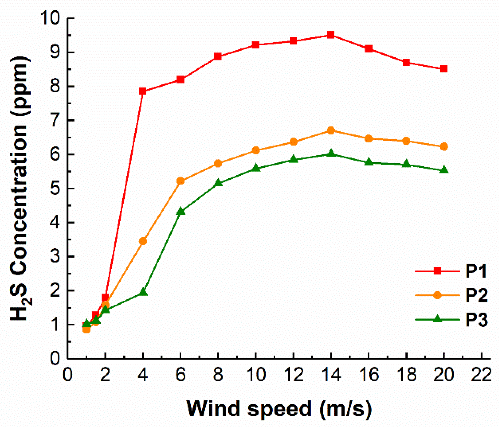
3.3. H2S Dispersion Simulation with Different Wind Speeds

Having wind speeds from 1 m/s to 20 m/s as the variable, the simulated H2S plumes were shown in Figure 5 and Figure 6. The legend shows the H2S concentration fraction of the initial concentration Q, which was the initial H2S concentration above the sewage pool closing to the water surface.
The change of H2S concentration fraction revealed the dispersion tendency of H2S. Generally, with wind speed increasing, H2S concentration declined with height increase in y direction, influenced range enlarged with the increase of distance in x direction, and the H2S plume eventually stabilized at a limit height about 3 m during the wind speed changes. The whole plume shape was consistent with the report of Abdullah and Weiming [31] about leaked gas having the same, or similar, density as ambient air. For more details, the research range was divided into two parts. Region 1 was the range above the sewage pool (x coordinate from −10 m to 10 m), and region 2 was the rest (x coordinate from 10 m to 25 m).
Region 1 mainly observed the wind speed influence on H2S emission. It was evaluated by the H2S high concentration range (H2S concentration above 0.5Q) change. Before 2 m/s, the turbulence caused by wind was not strong enough to produce a big mass transfer coefficient for strong mass transfer. So, the H2S high concentration range was small. At the outlet of the tank, the H2S concentration reached 0.9Q. That is because the velocity ratio between odorous compounds velocity at the source outlet and wind speed was small [32]. The H2S compounds tended to disperse vertically upward. This characteristic was also noticed in Figure 7, where, before 2 m/s, the H2S concentrations at P1, P2, and P3 were close. However, from 4 m/s, the stronger turbulence improved the mass transfer, and the vertical dispersion was improved. Comparing the H2S plumes of different wind speeds in Figure 5 and Figure 6, the H2S emission was strengthened with wind speed, increasing from 2 m/s to 10 m/s. High wind speeds let the ambient air have more power to carry the H2S climbing up, presenting a larger influence height.
Surprisingly, the growth trend of the high-concentration H2S range in region 1 changed in high wind speed condition. When the wind speeds were faster than 10 m/s, the high-concentration H2S influence range shrank. This phenomenon was studied in depth, and the reason was found to be the change of flow field (Figure 8).
In the three cases (4 m/s, 10 m/s, and 18 m/s) in Figure 8, the slope of streamline above region 1 was positive, which meant air flowed upwards. The slope was minimum at 4 m/s and maximum at 10 m/s. The slope of 18 m/s was in the middle, which was slightly smaller than 10 m/s (Figure 9). The characteristics of air flow were exactly the reason why the influence range of high-concentration H2S first increased and then decreased.
Region 2 mainly observed the influence of wind speed on the H2S dispersion. When the wind speed was under 2 m/s, due to the small amount of H2S emission, the whole region 2 was H2S low-concentration range (H2S concentration under 0.5Q). H2S tended to disperse perpendicularly to the jet direction because the horizontal velocity was also small. Additionally, the edge of the plume was unsmooth. With wind speed augmenting to 4 m/s, the H2S concentration changed quickly. This concentration rapidly changed, due to wind speed rise, which was also illustrated in Shen’s research [33]. It was displayed by the concentration gradient in Figure 7. Anyway, the plume edge began to be smooth. It meant that more H2S dispersed down-wind, instead of flying up, which increased the H2S fraction in region 2. With the further increase of wind speed, the height of the influence range gradually rose again and stabilized at about 3 m under 8 m/s. After 10 m/s, the H2S influence range was basically unchanged. This phenomenon was also found in the outdoor H2S dispersion study of a landfill [34]. The whole H2S influence range fluctuation in Figure 6 and the streamlines state in Figure 8 explain that, as the distance between the observation point and the leak source increased, the influence of air flow on the distribution of H2S became more obvious, which was consistent with the report of Majid et al [35].
Meanwhile, the H2S plume structure was also changed. With the increase of wind speed from 4 m/s to 12 m/s, the thickness of each concentration layer increased. However, this trend reversed from 14 m/s. As the wind speed continued to increase, the layers whose fractions were higher than 0.5Q became thinner, and other layers whose fractions were smaller than 0.5Q became thicker. The H2S distribution changed because of the flow field change, which was the same as region 1 (Figure 9). In the three cases, focusing on the slopes of streamlines in region 2, it was noticeable that the changes in characteristics were similar to the slopes in region 1. Using k to represent the slope, we could obtain that k4 < k18 < k10. The change of streamline slope conducted the H2S layer thickness change.

3.4. Safe Distance for Outdoor Sedimentation Tank

In certain industries, such as landfills, sewage treatment plants, and animal husbandry, workers face a higher risk of H2S exposure. Therefore, H2S occupational exposure is highly regarded, and relevant laws and regulations have been formulated in various countries [36,37].
As mentioned above, China specifies a H2S maximum allowable concentration (MAC), which is 10 mg/m3. Uniformly converting the units of H2S MAC to ppm for data analysis, 10 mg/m3 corresponded to 6.9 ppm. The initial measured max concentration Q was 13.34 ppm. So, the MAC of H2S equaled 0.54Q. Hence, an area having H2S concentration fraction higher than 0.54Q could be regarded as the unsafe region.
The area bounded by a 0.54Q curve and the x-axis was an unsafe region in Figure 10. The unsafe region of 2 m/s was about 11 m long and 0.5 m high, which was the distance away from the office monitoring point P2. As for lower wind speed, such as 1 m/s and 1.5 m/s, whose unsafe region were supposed to be smaller than 2 m/s, being similar with the H2S plume change in region 1, the unsafe region first developed and then shrank with wind speed increase. According to the onsite data, mostly the wind speed in Jingzhou city was under 8 m/s, whose corresponding safe region was 17.2 m long and 1.5 m height. This is the most basic distance for workers to be safe, but the general safe region was supposed to be larger than 17.2 m. Under 12 m/s, the unsafe region reached its maximum range, which was 19.5 m long and 1.7 m height. With wind speed higher than 12 m/s, the unsafe region began to shrink.
Anyway, analyzing the partial enlarged drawing in Figure 10, it was found that the slope of H2S concentration under different wind speeds had the same characteristics as the streamlines of different wind speeds. The unsafe region border slope before 10 m/s was always greater than the slope after 10 m/s, which meant H2S dispersed further down-wind after 10 m/s. It was concluded that, under the worst environment conditions of 12 m/s, the safe distance was over about 20 m long and 1.8 m height. Therefore, the office at point 2 was suitable for workers only when the wind speed was less than 2 m/s. Additionally, the sidewalk at point 3 could be used as a daily road. In summary, for this model scenario, a work office was better be set at least 10 m away from the wastewater pool (down-wind direction). The adjusted sewage pool model is shown below in Figure 11.

4. Conclusions

For surface source unorganized H2S dispersion modeling, RNG is the most suitable k-ε turbulence model that most closely matches the experimental measurements. Using the RNG model to explore the influences of temperature and wind speed on H2S dispersion, the results show that temperature change indeed leads to different H2S production and different H2S concentration at the monitoring points, but the effect is much smaller than wind speed for H2S dispersion. The different wind speed changes the flow field. Taking the wind speed of 12 m/s as the dividing line, H2S dispersion shows two states: enhanced (less than 12 m/s) and unchanged (more than 12 m/s).
In this case, the CFD simulation provides a visualization for H2S dispersion at short distance outdoors. Between 288 K to 303 K, the H2S concentration outside the sewage sedimentation tank does not reach the occupational exposure limit when the wind speed is less than 2 m/s. However, when the wind speed increases from 4 m/s to 12 m/s, the safety distance increases from 7 m to the maximum of 10 m. Therefore, for the sewage sedimentation tank with sewage treatment capacity less than or equal to 10 m3/h, it is recommended that workshops or offices be built 10 m away from the pollution source. This guidance would have value for practical industrial environment layouts.

Author Contributions

Conceptualization, W.M. and J.G.; methodology, Z.Z.; validation, J.G.; investigation, Z.Z.; writing—original draft preparation, J.G.; writing—review and editing, W.M. and W.D.; visualization, W.D.; supervision, L.L.; funding acquisition, L.L. All authors have read and agreed to the published version of the manuscript.

Funding

This research was funded by the National Key R&D Program of China, grant number 2019YFC0214303.

Data Availability Statement

Not applicable.

Conflicts of Interest

The authors declare no conflict of interest.

References

  1. Li, W.; Yang, W.; Li, J. Characterization and prediction of odours from municipal sewage treatment plant. Water Sci. Technol. 2018, 2017, 762–769. [Google Scholar] [CrossRef] [PubMed]
  2. Guarrasi, J.; Trask, C.; Kirychuk, S. A Systematic Review of Occupational Exposure to Hydrogen Sulfide in Livestock Operations. J. Agromed. 2015, 20, 225–236. [Google Scholar] [CrossRef] [PubMed]
  3. Colomer, F.L.; Morató, H.E.; Iglesias, E.M. Estimation of hydrogen sulfide emission rates at several wastewater treatment plants through experimental concentration measurements and dispersion modeling. J. Air Waste Manag. Assoc. 2012, 62, 758–766. [Google Scholar] [CrossRef] [PubMed]
  4. Liu, Y.; Lu, W.; Wang, H.; Gao, X. Odor impact assessment of trace sulfur compounds from working faces of landfills in Beijing, China. J. Environ. Manag. 2018, 220, 136–141. [Google Scholar] [CrossRef]
  5. Yalamanchili, C.; Smith, M.D. Acute hydrogen sulfide toxicity due to sewer gas exposure. Am. J. Emerg. Med. 2008, 26, 518.e5–518.e7. [Google Scholar] [CrossRef]
  6. Jiang, Q.; Li, T.; He, Y.; Wu, Y.; Zhang, J.; Jiang, M. Simultaneous removal of hydrogen sulfide and ammonia in the gas phase: A review. Environ. Chem. Lett. 2022, 20, 1403–1419. [Google Scholar] [CrossRef]
  7. Bu, H.; Carvalho, G.; Yuan, Z.; Bond, P.; Jiang, G. Biotrickling filter for the removal of volatile sulfur compounds from sewers: A review. Chemosphere 2021, 277, 130333. [Google Scholar] [CrossRef]
  8. Jiang, Z.A.; Wang, Y.P.; Men, L.G. Ventilation control of tunnel drilling dust based on numerical simulation. J. Cent. South Univ. 2021, 25, 1342–1356. [Google Scholar] [CrossRef]
  9. Nuvolone, D.; Petri, D.; Pepe, P.; Voller, F. Health effects associated with chronic exposure to low-level hydrogen sulfide from geothermoelectric power plants. A residential cohort study in the geothermal area of Mt. Amiata in Tuscany. Sci. Total Environ. 2019, 659, 973–982. [Google Scholar] [CrossRef] [PubMed]
  10. Haouzi, P.; Tubbs, N.; Cheung, J.; Judenherc-Haouzi, A. Methylene Blue Administration During and After Life-Threatening Intoxication by Hydrogen Sulfide: Efficacy Studies in Adult Sheep and Mechanisms of Action. Toxicol. Sci. 2019, 168, 443–459. [Google Scholar] [CrossRef] [PubMed]
  11. Selene, C.H.; Chou, J. Concise International Chemical Assessment Document 53: Hydrogen sulfide: Human health aspects. In IPCS Concise International Chemical Assessment Documents; World Health Organization: Geneva, Switzerland, 2003; p. 53. [Google Scholar]
  12. GBZ 2.1-2019; Occupational Exposure Limits for Hazardous Agents in the Workplace—Part 1: Chemical Hazardous Agents. Available online: http://www.nhc.gov.cn/wjw/pyl/202003/67e0bad1fb4a46ff98455b5772523d49.shtml (accessed on 13 September 2022).
  13. Walewska, A.; Szewczyk, A.; Koprowski, P. Gas Signaling Molecules and Mitochondrial Potassium Channels. Int. J. Mol. Sci. 2018, 19, 3227. [Google Scholar] [CrossRef] [PubMed] [Green Version]
  14. Somma, R.; Granieri, D.; Troise, C.; Terranova, C.; De Natale, G.; Pedone, M. Modelling of hydrogen sulfide dispersion from the geothermal power plants of Tuscany (Italy). Sci. Total Environ. 2017, 583, 408–420. [Google Scholar] [CrossRef] [PubMed]
  15. Moreno-Silva, C.; Calvo, D.C.; Torres, N.; Ayala, L.; Gaitán, M.; González, L.; Rincón, P.; Susa, M.R. Hydrogen sulphide emissions and dispersion modelling from a wastewater reservoir using flux chamber measurements and AERMOD® simulations. Atmos. Environ. 2020, 224, 117263. [Google Scholar] [CrossRef]
  16. Gulia, S.; Kumar, A.; Khare, M. Performance evaluation of CALPUFF and AERMOD dispersion models for air quality assessment of an industrial complex. J. Sci. Ind. Res. 2015, 74, 302–307. [Google Scholar]
  17. Wu, C.; Yang, F.; Brancher, M.; Liu, J.; Qu, C.; Piringer, M.; Schauberger, G. Determination of ammonia and hydrogen sulfide emissions from a commercial dairy farm with an exercise yard and the health-related impact for residents. Environ. Sci. Pollut. Res. 2020, 27, 37684–37698. [Google Scholar] [CrossRef]
  18. Asadollahfardi, G.; Mazinani, S.; Asadi, M.; Mirmohammadi, M. Mathematical and experimental study of hydrogen sulfide concentrations in the Kahrizak landfill, Tehran, Iran. Environ. Eng. Res. 2019, 24, 572–581. [Google Scholar] [CrossRef]
  19. Zhang, B.; Chen, G. Hydrogen Sulfide Dispersion Consequences Analysis in Different Wind Speeds: A CFD Based Approach. In Proceedings of the International Conference on Energy and Environment Technology, Washington, DC, USA, 16–18 October 2009; pp. 365–368. [Google Scholar]
  20. Lin, X.; Barrington, S.; Gong, G.; Choinière, D. Simulation of odour dispersion downwind from natural windbreaks using the computational fluid dynamics standard k-ε model. Can. J. Civ. Eng. 2009, 36, 895–910. [Google Scholar] [CrossRef]
  21. Tominaga, Y.; Stathopoulos, T. Numerical simulation of dispersion around an isolated cubic building: Comparison of various types of k-ε models. Atmos. Environ. 2009, 43, 3200–3210. [Google Scholar] [CrossRef]
  22. Moen, A.; Mauri, L.; Narasimhamurthy, V.D. Comparison of k-ε models in gaseous release and dispersion simulations using the CFD code FLACS. Process. Saf. Environ. Prot. 2019, 130, 306–316. [Google Scholar] [CrossRef]
  23. Abdul-Wahab, S.A.; Chan, K.; Elkamel, A.; Ahmadi, L. Effects of meteorological conditions on the concentration and dispersion of an accidental release of H2S in Canada. Atmos Environ. 2014, 82, 316–326. [Google Scholar] [CrossRef]
  24. Godoi, A.; Grasel, A.M.; Polezer, G.; Brown, A.; Potgieter-Vermaak, S.; Scremim, D.C.; Yamamoto, C.I.; Godoi, R.H.M. Human exposure to hydrogen sulphide concentrations near wastewater treatment plants. Sci. Total Environ. 2018, 610–611, 583–590. [Google Scholar] [CrossRef] [PubMed]
  25. Saeed, M.; Yu, J.; Abdalla, A.A.A.; Zhong, X.-P.; Ghazanfar, M.A. An assessment of k-ε turbulence models for gas distribution analysis. Nucl. Sci. Tech. 2017, 28, 146. [Google Scholar] [CrossRef]
  26. Mirzaei, F.; Mirzaei, F.; Kashi, E. Turbulence Model Selection for Heavy Gases Dispersion Modeling in Topographically Complex Area. J. Appl. Fluid. Mech. 2019, 12, 1745–1755. [Google Scholar] [CrossRef]
  27. Ben Ramoul, L.; Korichi, A.; Popa, C.; Zaidi, H.; Polidori, G. Numerical study of flow characteristics and pollutant dispersion using three RANS turbulence closure models. Environ. Fluid. Mech. 2019, 19, 379–400. [Google Scholar] [CrossRef]
  28. Lateb, M.; Masson, C.; Stathopoulos, T.; Bédard, C. Comparison of various types of k–ε models for pollutant emissions around a two-building configuration. J. Wind. Eng. Ind. Aerodyn. 2013, 115, 9–21. [Google Scholar] [CrossRef] [Green Version]
  29. Zwain, H.M.; Nile, B.K.; Faris, A.M.; Vakili, M.; Dahlan, I. Modelling of hydrogen sulfide fate and emissions in extended aeration sewage treatment plant using TOXCHEM simulations. Sci. Rep. 2020, 10, 22209. [Google Scholar] [CrossRef] [PubMed]
  30. Nagaraj, A.; Sattler, M.L. Correlating emissions with time and temperature to predict worst-case emissions from open liquid area sources. Air Repair 2005, 55, 1077–1084. [Google Scholar] [CrossRef] [PubMed] [Green Version]
  31. Alakalabi, A.; Liu, W. Numerical investigation into the effects of obstacles on heavy gas dispersion in the atmosphere. In Proceedings of the XII International Conference on Computational Heat, Mass and Momentum Transfer (ICCHMT 2019), Preston, UK, 8 November 2019. [Google Scholar]
  32. Maïzi, A.; Dhaouadi, H.; Bournot, P.; Mhiri, H. CFD prediction of odorous compound dispersion: Case study examining a full scale waste water treatment plant. Biosyst. Eng. 2010, 106, 68–78. [Google Scholar] [CrossRef]
  33. Shen, S.; Wu, B.; Xu, H.; Zhang, Z.-Y. Assessment of Landfill Odorous Gas Effect on Surrounding Environment. Adv. Civ. Eng. 2020, 2020, 8875393. [Google Scholar] [CrossRef]
  34. Feng, Y.; Eun, J.; Moon, S.; Nam, Y. Assessment of gas dispersion near an operating landfill treated by different intermediate covers with soil alone, low-density polyethylene (LLDPE), or ethylene vinyl alcohol (EVOH) geomembrane. Environ. Sci. Pollut. Res. 2022, 1–16. [Google Scholar] [CrossRef]
  35. Bayatian, M.; Azari, M.R.; Ashrafi, K.; Jafari, M.J.; Mehrabi, Y. CFD simulation for dispersion of benzene at a petroleum refinery in diverse atmospheric conditions. Environ. Sci. Pollut. Res. 2021, 28, 32973–32984. [Google Scholar] [CrossRef] [PubMed]
  36. List of Highly Hazardous Chemicals, Toxics and Reactives (Mandatory). Available online: https://www.osha.gov/laws-regs/regulations/standardnumber/1910/1910.119AppA (accessed on 13 September 2022).
  37. Costigan, M.G. Hydrogen sulfide: UK occupational exposure limits. Occup. Environ. Med. 2003, 60, 308–312. [Google Scholar] [CrossRef] [PubMed]
Figure 1. (a) The onsite view of the washing sewage sedimentation tank; (b) The 3D model of the onsite view; (c) The CFD model of the onsite view; (d) The schematic diagram of monitoring points. The numbers in parentheses represent x, y, z three-dimensional coordinates of monitoring points.
Atmosphere 13 01822 g001
Figure 2. Onsite data of H2S at 1.5 m height. The dotted line is the occupational exposure standard for H2S in China, which is 10 mg/m3 = 6.9 ppm.
Atmosphere 13 01822 g002
Figure 3. Validation of Realizable, RNG, and Standard model.
Atmosphere 13 01822 g003
Figure 4. H2S concentration at P1, P2, and P3 (0 m, 4 m, 11 m), with the temperature change (from 288 K to 303 K). The wind speed was constant at 4 m/s.
Atmosphere 13 01822 g004
Figure 5. H2S plume of wind speed 1 m/s, 1.5 m/s, and 2 m/s, controlling temperature at 298 K.
Atmosphere 13 01822 g005
Figure 6. H2S plume of wind speed changing from 4 m/s to 20 m/s, controlling temperature at 298 K.
Atmosphere 13 01822 g006
Figure 7. H2S concentration at P1, P2, and P3 with wind speed change only (from 2 m/s to 20 m/s). The temperature was a constant at 298 K.
Atmosphere 13 01822 g007
Figure 8. Streamline graphics of wind speed 4 m/s, 10 m/s, and 18 m/s case. The diagonal line in the dotted box represents the slope at the right end of the streamline in the box.
Atmosphere 13 01822 g008
Figure 9. Slope comparation of streamlines in region 1 and region 2 in the three cases (4 m/s, 10 m/s, and 18 m/s).
Atmosphere 13 01822 g009
Figure 10. Unsafe regions where H2S concentration was higher than 10 mg/m3.
Atmosphere 13 01822 g010
Figure 11. Modified model of building layout near automobile sewage pool.
Atmosphere 13 01822 g011
Table 1. Collection parameters of each measurement in experimental scene.
Measurement
No.
Collection DateSampling
Locations
TemperatureWind Speed
121 September 2020P1, P2, P3302.5–303.3 K3.2–4.6 m/s
28 March 2021P1, P2, P3287.8–288.4 K15.8–16.2 m/s
Table 2. H2S emission rate at different temperatures and wind speeds.
Wind Speed (m/s)Temperature (K)H2S Mass Flow Rate (kg/s)
1.02881.50
1.52881.51
2.02881.62
4.02882.18
2932.23
2982.29
3032.35
6.02882.62
8.02883.07
10.02883.49
12.02883.88
14.02884.25
16.02884.61
18.02884.95
20.02885.29
Table 3. Mean value, mean deviation, and ratio of mean deviation to mean value of H2S concentration with different temperatures at P1, P2, and P3.
H2S Concentration (ppm)P1P2P3
Mean value7.883.481.45
Mean deviation0.0550.0630.051
Ratio0.7%1.8%3.5%
Publisher’s Note: MDPI stays neutral with regard to jurisdictional claims in published maps and institutional affiliations.

