Article

Multitemporal Analysis of the Influence of PM10 on Human Mortality According to Urban Land Cover

by
Laura Marcela Ochoa-Alvarado
1,
Carlos Alfonso Zafra-Mejía
1,* and
Hugo Alexander Rondón-Quintana
2
1
Grupo de Investigación en Ingeniería Ambiental—GIIAUD, Facultad del Medio Ambiente y Recursos Naturales, Universidad Distrital Francisco José de Caldas, Carrera 5 Este # 15–82, Bogotá E-111711, Colombia
2
Ingeniería Topográfica, Facultad del Medio Ambiente y Recursos Naturales, Universidad Distrital Francisco José de Caldas, Carrera 5 Este # 15–82, Bogotá E-111711, Colombia
*
Author to whom correspondence should be addressed.
Atmosphere 2022, 13(12), 1949; https://doi.org/10.3390/atmos13121949
Submission received: 29 October 2022 / Revised: 17 November 2022 / Accepted: 20 November 2022 / Published: 23 November 2022
(This article belongs to the Special Issue Air Pollution, Air Quality and Human Health)

Abstract

:
High urbanization and a consequent change in land cover can lead to a deterioration in air quality and generate impacts on public health. The objective of this paper is to provide a multitemporal analysis of the influence of particulate matter ≤ 10 μm (PM10) on human mortality from the land cover variation in a Latin American megacity. Six monitoring stations (monitoring daily PM10 concentration, increases in daily mortality (IDM), and land cover) were established throughout the megacity. The results suggest that for every 10% increase in vegetation cover, the daily PM10 concentration and IDM decreases by 7.5 μg/m3 and 0.34%, respectively. Moreover, it is evident that the monitoring station with the lowest vegetation cover (8.96 times) shows an increase of 1.56 times and 4.8 times in the daily PM10 concentration and IDM, respectively, compared with the monitoring station with the highest vegetation cover (46.7%). It is also suggested that for each increase of 100 inhabitants/hectare in population density, the daily PM10 concentration and IDM increases by 9.99 µg/m3 and 0.45%, respectively. Finally, the population densification of the megacity possibly implies a loss of vegetation cover and contributes to the increase in PM10 and IDM.

1. Introduction

Air pollution is a global problem that can generate negative environmental effects and harm human health [1,2,3]. According to the World Health Organization (WHO), the rate of mortality attributable to urban air pollution in Latin America and the Caribbean is seven deaths per 100,000 inhabitants, with exposure to particulate matter ≤ 10 μm (PM10) being one of the main influencing factors [4]. Indeed, most pollutants come from anthropogenic sources, such as emissions from vehicles and industrial processes [5]. Air pollution is also associated with urbanization and rapid economic development [6]. In urban areas that measure air pollution levels, WHO identified that more than 80% of inhabitants were exposed to concentrations that exceeded their guideline values [5].
Changes in land use and, consequently, changes in surface cover are often associated with urban expansion. This expansion leads to the loss of ecosystems and the decline of green areas and impacts the environmental conditions of cities [7]. Land cover is then conditioned by urbanization, which is a process that alters the size, structure, and growth of cities in response to population explosion and leads to lasting challenges in air quality control [8]. Thus, in the study megacity (Bogotá D.C., Colombia), high urbanization may be associated with a deterioration in air quality and impacts on public health [9,10]. Epidemiological studies have identified that urban air pollution by PM2.5 was associated with increased risks of human morbidity and mortality [11]. The PM pollution varies in time and space and is dominated by differences in geographic conditions, such as topography, meteorology, land use, urbanization, and industrialization [2]. In the context of urban and environmental studies, it was demonstrated that PM2.5 pollution was strongly related to the pattern of microscale land cover change, and it was also suggested that optimizing this pattern could contribute to air pollution mitigation [12,13]. Therefore, analyzing the dynamics of PM10 and PM2.5 pollution in relation to land cover and its impact on human health will facilitate a deeper understanding of the air quality problem, framed in the interaction between human activities and urban environment.
The temporal association of air pollution with human health has been evaluated in numerous studies (e.g., [14,15]). Epidemiological studies suggested that short-term exposure to air pollution was associated with increased mortality from respiratory and cardiovascular diseases [16,17]. Correlations have also been identified with the increase in the rates of visits to emergency departments for respiratory and cardiovascular issues, and with the number of hospitalizations [18]. In Bogotá D.C., it was estimated that PM2.5 contributed to more than 10% of deaths [9]. The PM10 impacts on public health also generated economic and social costs that were mainly attributed to premature deaths, higher health care expenditures, and productivity losses [19]. A study developed by Aguiar-Gil et al. [20] in the metropolitan area of Aburra Valley (Colombia) reported the following cases of deaths in adults that were attributable to PM2.5 pollution: 1971 cases from all causes (95% CI: 1363–2559); 194 cases from lung cancer (95% CI: 92–284); and 932 cases from ischemic heart disease (95% CI: 791–1064). These authors also reported that in the case of implementing 100% of the measures to prevent and control emissions from motor vehicles by 2030, as defined in the city’s air quality plan, 55.7% of adult deaths attributable to PM2.5 could be avoided. Rodríguez-Villamizar et al. [18] also reported, when considering respiratory and circulatory diseases in five cities in Colombia, that adverse effects were statistically more significant in models with zero days of delay in exposure. This suggested that the negative impacts on human health of air pollutant mixtures were more significant in the short term. These researchers reported that mixtures of traffic-related air pollutants (NO2 + CO + PM10) had a greater combined effect on human morbidity related to the circulatory and respiratory systems.
Urban growth was associated with air pollution because of its dynamics of densifying cities [21]. To describe the relationship between land use and the air pollution level, for example, regression models have been developed in European, American, and Asian cities. In a study conducted in Shanghai (China), the following factors were identified as having significant explanatory value for a PM2.5 pollution model: residential area, distance to coast, industrial area, urban district, and road density (R2 = 0.88) [12]. Indeed, the detected factors in each case were associated with different types of predominant land cover. In Shanxi Province (China), a geographically weighted regression model was also developed, in which the researchers identified that the decreasing order in PM2.5 concentration for the different land covers considered was as follows: land with constructions (buildings and roads) > unused land > water bodies > cropland > grasslands > forests [7].
The main objective of this paper is to provide a multitemporal analysis of the influence of PM10 on human mortality from the land cover variation in Bogotá D.C. Six monitoring stations were established throughout the megacity. The multitemporal analysis was performed during the period from 2008 to 2018. The time scales of this study’s analysis were hourly, daily, and monthly. In the context of urban air pollution, this study provides increased knowledge in relation to the following aspects: (1) the temporal behavior of daily PM10 in Bogotá D.C.;(2) the impact of daily PM10 on urban public health (e.g., the increase in human mortality); and (3) the relationship between urban land cover and PM10 pollution. Finally, PM10 was used as a size fraction indicative of the increase in daily mortality (IDM) according to land cover, because in Bogotá D.C. the time series of PM2.5 concentrations were short and scarce. Indeed, this did not allow a detailed spatiotemporal analysis for PM2.5 in the context of this study.

2. Materials and Methods
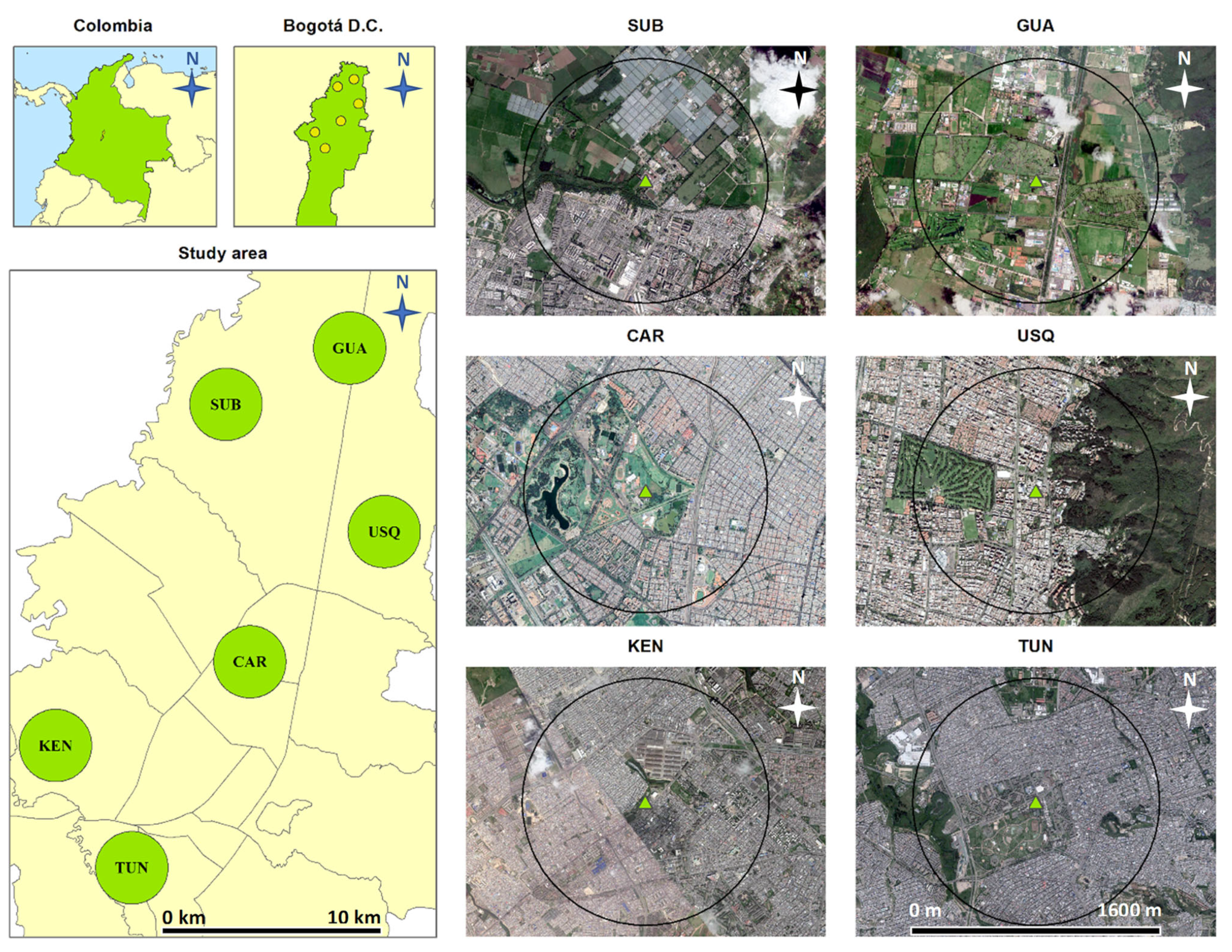
2.1. Study Site

Six stations were established to monitor background PM10 concentrations, which were distributed throughout the megacity. The area of influence considered for each monitoring station, based on its physical location, covered a radius of 1600 m (Figure 1). The selected monitoring stations were identified as follows: Centro de Alto Rendimiento (CAR), Kennedy (KEN), Guaymaral (GUA), Suba (SUB), Tunal (TUN), and Usaquén (USQ). These monitoring stations were in five locations of the megacity (Barrios Unidos, Kennedy, Suba, Tunjuelito, and Usaquén). In the megacity, the population of approximately 8 million inhabitants was concentrated, and increased to more than 10 million with the inclusion of its metropolitan area. The megacity was established as the main geographical, political, industrial, economic, and cultural center of Colombia [22]. Bogotá D.C. is located near the Equator. Thus, there are no seasons such as those observed at higher latitudes. The climate of the study sites was tropical mountain, with wide hourly variations in temperature (between 7.2 °C and 19 °C). On average, the inventory of PM10 emissions showed the following contributions for 2018: mobile sources = 7.62%, fixed sources = 1.06%, natural and forest sources = 0.11%, and resuspended particulate matter = 91.2% [23]. Table 1 shows the main characteristics of the study areas that were established.

2.2. Information Collection

The information collected on PM10 corresponded to hourly values between 1 January 2008, and 31 December 2018. The information was obtained from six monitoring stations that measured background concentrations. In other words, the established stations were characterized by not being influenced by pollution sources, such as vehicular traffic and industries. The equipment for the measurement of PM10 concentration operated under the guidelines established in Title 40 of the Code of Federal Regulations of the U.S. Environmental Protection Agency (U.S. EPA) [24]. These devices operated using the beta ray attenuation method. The precision of the equipment used was as follows: ±5 μg/m3 for concentrations below 80 μg/m3 and 7% for concentrations above 80 μg/m3 (Appendix J: Part 50, Title 40 of the CFR) [24].
The IDM was calculated from the results of the study conducted by Blanco et al. [4] for PM10 in Bogotá D.C. Those researchers performed a time series analysis from 1998 to 2006 to study the association between daily mortality and acute PM10 exposure. On average, the results of that study indicated that the percentage change in mortality risk for all ages and causes was 0.57% (95% CI: 0.25–0.89%, minimum = 0.08%, and maximum = 1.06%) for each 10 μg/m3 increase in PM10 concentration during the same day of exposure. This was according to the international classification of diseases established by WHO [25]. Other studies (e.g., [10]) also used the findings of Blanco et al. [4] to facilitate the inclusion in their analyses of the daily mortality risk due to PM10 exposure.
The land cover was determined using high-resolution Quickbird satellite images (spatial resolution = 2.50 m) between 2008 and 2018, which were freely downloaded from Google Earth Pro V.7.3 software. Information on the different types of land cover was collected during the study period; then, data were averaged for each monitoring station (radius = 1600 m). It was assumed that there were no significant changes in land cover of the megacity during the study period. On average, vegetation, impermeable, water bodies, and bare land covers changed by −0.49%, 6.07%, −0.03%, and −3.04%, respectively. Land cover was identified using supervised classification, applying the maximum likelihood method, and employing ArcGIS Desktop V.10.4.1. software [26]. In this study, the following types of urban land covers were considered [7,27]: (i) vegetation (trees, grasslands, and crops), (ii) impermeable (buildings and roads), (iii) bare land (uncovered land and quarries), and (iv) water bodies (rivers, lakes, and wetlands). Finally, the urban population density reported by the Planning Secretariat of Bogotá D.C. was considered [28].

2.3. Information Analysis

The information analysis considered four phases. In the first phase, information on PM10 concentrations at each of the established monitoring stations was analyzed. A time series of hourly PM10 concentrations was generated at each station, which had a percentage of valid information greater than 75% [29]. From frequency histograms, it was confirmed that the data showed a positive asymmetry coefficient, and through a Kolmogorov–Smirnov test [30], the non-normal distribution of the data series was confirmed (p-value < 0.001). The correlation of data between monitoring stations was analyzed using Spearman’s coefficient (rs) [31]. A Tukey test determined the upper and lower limits in the time series of PM10 concentrations to detect the occurrence of outliers [32]. These outliers were then removed from the time series. The missing data in the time series were completed using the normal value ratio method, which enabled the estimation of a missing value when there were support stations that showed a similar temporal behavior as that observed at the study station [33]. Thus, combinations of three support stations that showed a Spearman correlation coefficient greater than 0.50 in relation to the station to be completed were used to complete each item of the missing data [34]. Moreover, daily PM10 concentrations (moving average for 24 h) were calculated to compare them with the limits established by the Colombian guideline (Resolution 2254 of 2017) [35] and with those established by the WHO Air Quality Guide [25]. In this study, the results were also analyzed under hourly, daily, and monthly time scales. This information was spatially represented in the megacity using Kriging’s geostatistical interpolation method [36] and ArcGIS Desktop V.10.4.1 software.
In the second phase, IDM was analyzed. The IDM for all ages and causes in the megacity under study was calculated. For this purpose, each item of daily PM10 concentration data was subtracted by 50 μg/m3 (the lower limit of calculation), because the total mortality increased from this reference value in response to prolonged exposure to daily PM10. This was according to a meta-analysis conducted by WHO [25]. The resulting negative data were adjusted to 0.0 μg/m3. Subsequently, IDM was calculated from the rate reported by Blanco et al. [4] for the city of Bogotá D.C., where for each 10 μg/m3 increase in daily PM10, the IDM increased 0.57% (linear model). In this study, in calculating the IDM, it was not assumed that an increase in population was associated with an increase in PM10 concentration. Indeed, PM10 concentrations were measured directly, over time (between 2008 and 2018), from the established monitoring stations. The results obtained were analyzed under the daily and monthly time scales. This information was spatially analyzed in the megacity applying the Kriging’s geostatistical interpolation method [36] and using ArcGIS Desktop V.10.4.1 software.
In the third phase, land cover information was analyzed. Buffer zones were established based on the physical location of each of the six selected monitoring stations (Figure 1). The radii of influence considered were the following [27]: 50 m, 100 m, 200 m, 400 m, 800 m, and 1600 m. In each of the areas of influence of the monitoring stations, the increase or decrease (%) in the land cover considered was evaluated [37].
In the fourth phase, a multitemporal analysis was carried out between 2008 and 2018 based on the results obtained in the previous phases. Initially, the multitemporal behavior (hourly, daily, and monthly) of PM10 concentrations was analyzed, and the concentrations were compared with respect to the limits established by the Colombian (Resolution 2254 of 2017) [35] and WHO [25] guidelines. The spatial behavior of PM10 concentrations during the months identified as those of highest risk (February, average PM10 = 59.8 μg/m3) and lowest risk (July, average PM10 = 41 μg/m3) was analyzed, based on the maps generated in the previous phases, using the Kriging’s geostatistical interpolation method [36]. Next, the daily influence of PM10 concentrations on mortality was analyzed through a multitemporal analysis of IDM for all causes and ages. The spatial behavior of IDM in the megacity was also analyzed. Finally, the land cover variation in the different areas of influence was studied using linear regression models [38]. Specifically, the correlation between the following variables was analyzed: (i) vegetation cover and daily PM10 concentrations, and (ii) population density and daily PM10 concentrations.

3. Results and Discussion

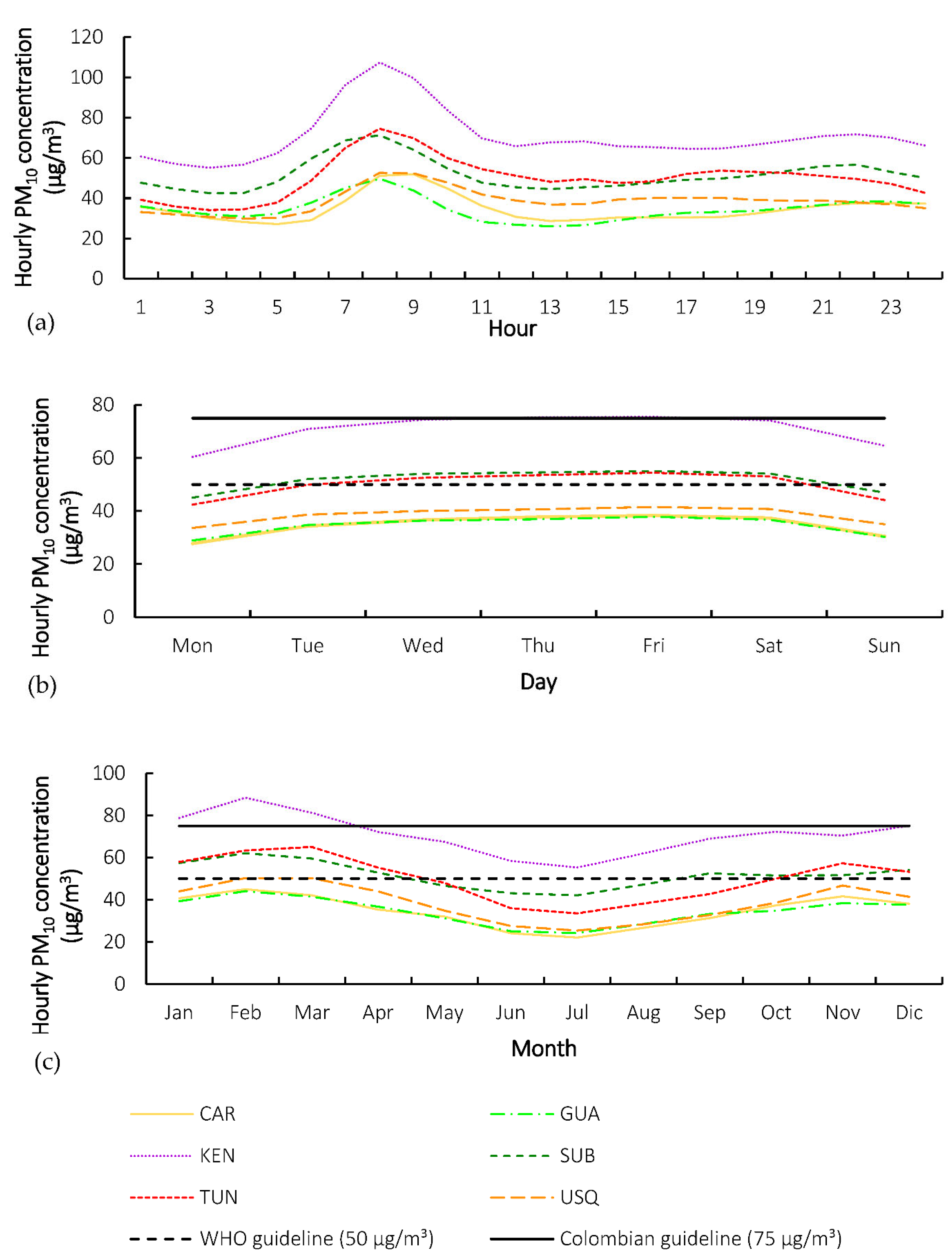
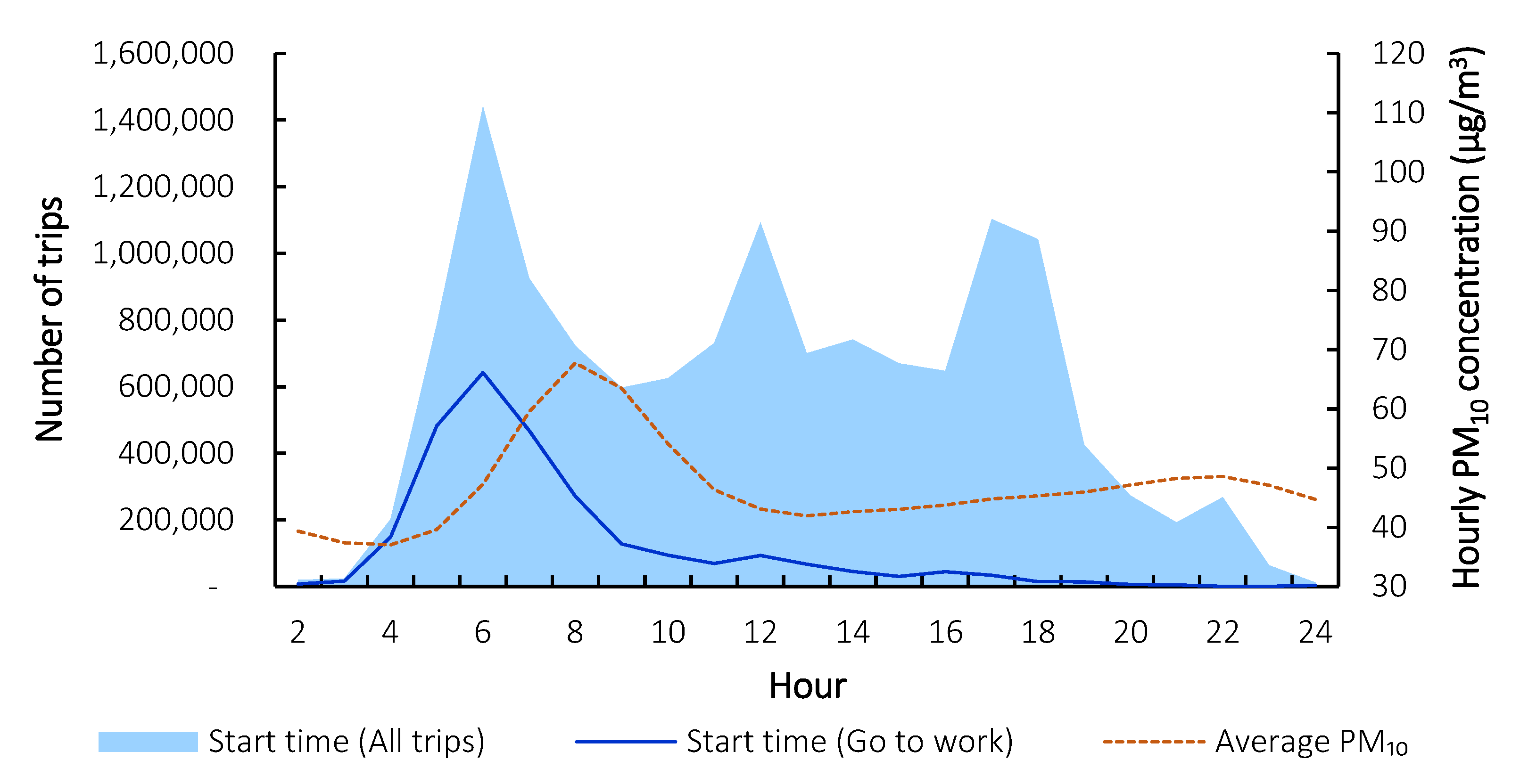
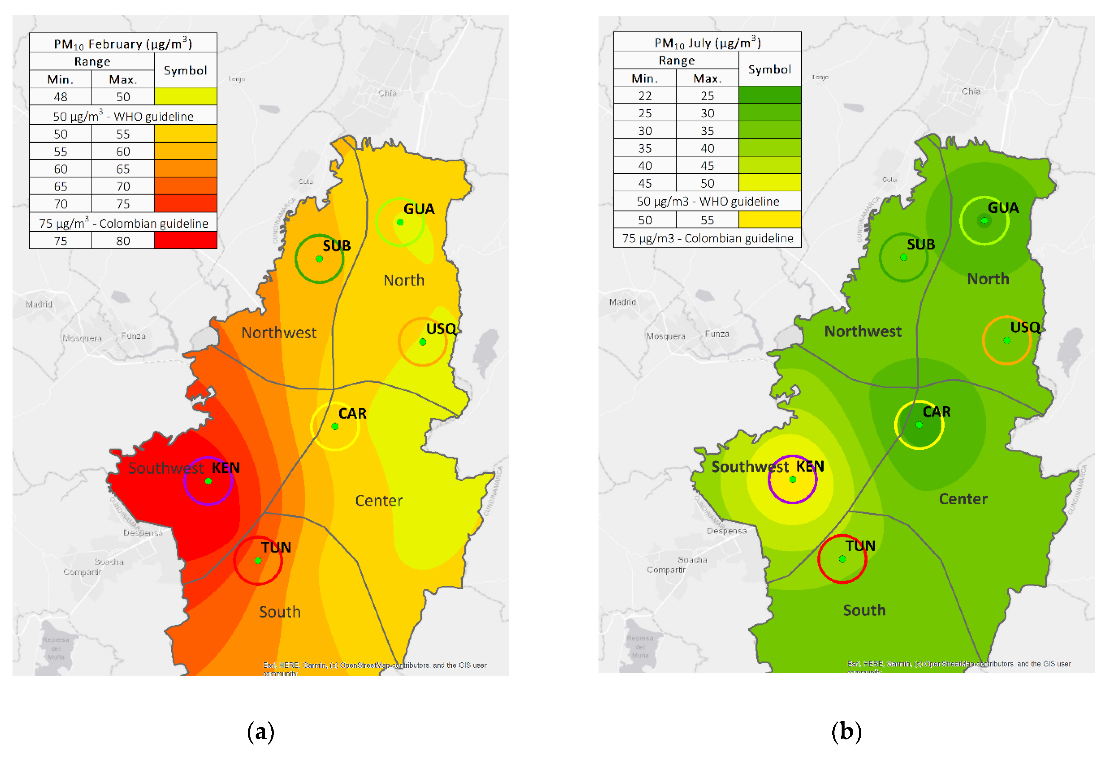
3.1. Spatiotemporal Analysis of PM10

The results showed that the hourly PM10 concentrations began to increase at 4:00 h, and at 8:00 h, the hourly concentration peak was observed. From this time, concentrations decreased to 12:00 h. Then, concentrations were relatively stable until 22:00 h, where a decrease in concentrations was observed again (Figure 2a). Similar results were obtained by Franceschi et al. [39], who reported that the hourly concentration peaks in the studied megacity were observed between 6:00 and 9:00 h. On average, the highest concentrations were observed at 8:00 h (67.8 μg/m3) and the lowest concentrations were observed at 4:00 h (31.7 μg/m3). The maximum hourly PM10 concentrations were 1.83 times higher than the lowest hourly concentrations observed. Nevertheless, there were comparatively extreme trends among the study stations that were established. For example, it was observed that during peak hour (8:00 h), the GUA station showed an average PM10 concentration of 49.7 μg/m3 and at the KEN station this concentration was 107.4 μg/m3 (2.16 times higher). The KEN station was the one that showed the highest daily concentrations during the study period (average = 70.8 μg/m3). In contrast, the CAR station was the one that showed the lowest daily PM10 concentrations during the study period (average = 34.6 μg/m3).
The above findings suggested that PM10 pollution peaks were possibly associated with the displacement of the inhabitants from their workplaces (via motor vehicles). This work displacement occurred between 5:00–9:00 h, according to the 2015 Mobility Survey conducted by the megacity [40]. A correlation analysis detected very strong associations between the number of work trips and hourly PM10 concentrations (rs = 0.904; p-value < 0.05). The previous analysis considered a two-hour delay for observed hourly PM10 concentrations. In this study, it was visualized that at 6:00 h the peak of work trips occurred in the megacity (642,369 trips), and two hours later (8:00 h), the PM10 concentration peak was observed (Figure 3). From the development of a linear regression model, it was detected that, on average, for every 100,000 trips there was an increase in the hourly PM10 concentration of 4.0 μg/m3. This was under the scenario of a two-hour delay (y = 4 × 10⁻⁵x + 42.3; x = number of hourly trips, y = hourly PM10 in μg/m3; R2 = 0.817). The previous analysis considered all observed hourly information. Considering only the information between 1:00 and 12:00 h, the time in which the concentration peaks were observed, a better correlation between these two variables was found (rs = 0.986; p-value < 0.05). In other words, for every 100,000 trips, the hourly PM10 concentration increased by 5.0 µg/m3 (y = 5 × 10⁻⁵x + 38.7; R2 = 0.973). Ramirez et al. [41] reported that motor vehicle-related emissions (combustion and resuspended PM) were the main PM10 source (≈50%) in the megacity. Finally, two additional peaks in the number of work trips (12:00 h and 17:00 h) were observed, which were not associated with increases in hourly PM10 concentrations. This PM10 trend could be associated with the hourly variation of the mixing–layer height. Studies have been carried out in the megacity that reported mixing–layer heights between 722 m and 1085 m during the hourly PM10 concentration peaks (8:00 h). Conversely, between 12:00 h and 17:00 h, these studies reported mixing–layer heights greater than 2500 m [10]. Therefore, the mixing–layer height possibly conditioned the PM10 dispersion.
The results showed that daily PM10 concentrations varied slightly during the first days of the week. However, comparatively greater variations were observed over the weekend. Average daily PM10 concentrations showed an increase from Monday to Wednesday (average = 23.4%), while from Wednesday to Saturday the increase was lower (average = 0.749%). Next, concentrations decreased from Saturday to Monday (average = 19.6%) (Figure 2b). This weekly behavior was possibly associated with the working-time model established in Bogotá D.C. [42]. During the week, the interval of greatest work intensity was reported from Wednesday to Saturday (average PM10 = 49.6 µg/m3) and the interval of least work intensity was from Sunday to Tuesday (average PM10 = 43.8 µg/m3). In relation to compliance with the limit established by the Colombian guideline (Resolution 2254 of 2017) [35], on average, all stations complied. This is because they recorded daily PM10 concentrations < 75 μg/m3, except in the KEN station, which from Thursday (75.3 μg/m3) to Friday (75.5 μg/m3) exceeded the established Colombian limit. In relation to the WHO guideline value for daily PM10 (50 μg/m3), the KEN station exceeded this value, on average, every day (60.4–75.5 μg/m3). The SUB (52–54.1 μg/m3) and TUN (50–53 μg/m3) stations also exceeded the WHO guideline value from Tuesday to Saturday. According to the observed concentrations that exceeded the WHO limit, the KEN station was the most critical during all days of the week (excess = 41.5%), followed by the SUB (excess = 7.88%, Tuesday to Saturday), and TUN (excess = 5.32%, Tuesday to Saturday) monitoring stations.
The monthly behavior of PM10 concentrations was similar in each of the established monitoring stations. The most critical interval was from January to March (average PM10= 57.7 µg/m3) and the least critical interval was from June to August (average PM10 = 42.6 µg/m3) (Figure 2c). The most critical month was February (average = 59.8 µg/m3) and the least critical month was July (average = 41 µg/m3). The results showed that PM10 concentrations were 1.35 times higher in February than those observed in July. This behavior could be influenced by the weather conditions of the megacity. On average, in the most critical interval, low rainfall (68.2 mm) and wind speeds (1.73 m/s) were observed. These climatic conditions were associated with the frequent occurrence of thermal inversion episodes, which prevented the development of upward air currents that dispersed air pollutants [43]. In the less critical interval, higher wind speeds (1.97 m/s) were observed, which probably facilitated the dispersion of air pollutants emitted from the megacity. Different studies also reported the negative correlation between wind speed and PM10 concentrations (e.g., [2,44]). This study was no exception. Monthly, a medium-to-strong negative correlation between wind speed and PM10 concentration was detected (rs = −0.667; p-value < 0.05). For each 1.0 m/s increase in wind speed, the PM10 concentration decreased by 54.2 μg/m3 (y = −34.2x + 107; x = wind speed in m/s, and y = monthly PM10 concentration in μg/m3; R2 = 0.445).
Monthly, the findings showed that PM10 concentrations in all monitoring stations complied with the limit established by the Colombian guideline, except for the KEN station (average = 81.5 μg/m3), during the most critical interval (January to March). The WHO guideline value was only complied with by the GUA, CAR, and USQ stations. The SUB and TUN stations only complied with the WHO guideline value during the least critical interval (June to August) and in May. Finally, the KEN station did not show monthly PM10 concentrations lower than the guideline value established by WHO. According to the information observed for monthly PM10 concentrations, it was possible to classify the monitoring stations according to their pollution degree, as follows: high pollution = KEN (59.6–75.5 µg/m3), medium pollution = TUN and SUB (43.6–59.6 µg/m3), and low pollution = CAR, GUA, and USQ (27.7–43.6 µg/m3).
The spatial variation of PM10 concentrations had a similar behavior, both in the most critical month (Figure 4a) and in the least critical month (Figure 4b). It was evident that the area of the megacity with the highest concentrations was the southwest (71.6 μg/m3 in February and 40.2 μg/m3 in July). Medium concentrations were observed in the northwestern and southern areas of the megacity (58 μg/m3 in February and 32.1 μg/m3 in July; 60.3 μg/m3 in February and 34.3 μg/m3 in July, respectively). Low concentrations were observed in the north (51.2 μg/m3 in February and 30.1 μg/m3 in July) and central (51.5 μg/m3 in February and 31.7 μg/m3 in July) areas. It was established that the Colombian guideline was complied with throughout the megacity during July, while in February the concentrations exceeded this limit in the southwestern zone (average exceedance = 6.67%; area = 4499 ha). In relation to the WHO guideline value, during July this limit was exceeded in the KEN station in the southwest (average excess = 10%; area = 734 ha). However, in February, only a part of the north–central zone (area = 15,516 ha) showed concentrations lower than the WHO guideline value. On average, the southwestern zone showed PM10 concentrations that were 1.36 times higher than those observed in the northern zone. This spatial behavior could be due, on the one hand, to the fact that the removal of this pollutant by wind action was not so efficient in the southwestern and southern areas of the megacity. On the other hand, in these areas there were covers of bare land, where the wind could resuspend the dust deposited on the urban surface. This possibly contributed to the increase in observed PM10 concentrations [45]. Moreover, as these areas are highly densified, an increase in PM10 could be generated due to the concentration of pollution sources and the possible reduction in wind speed due to the physical barriers constituted by the buildings [46].

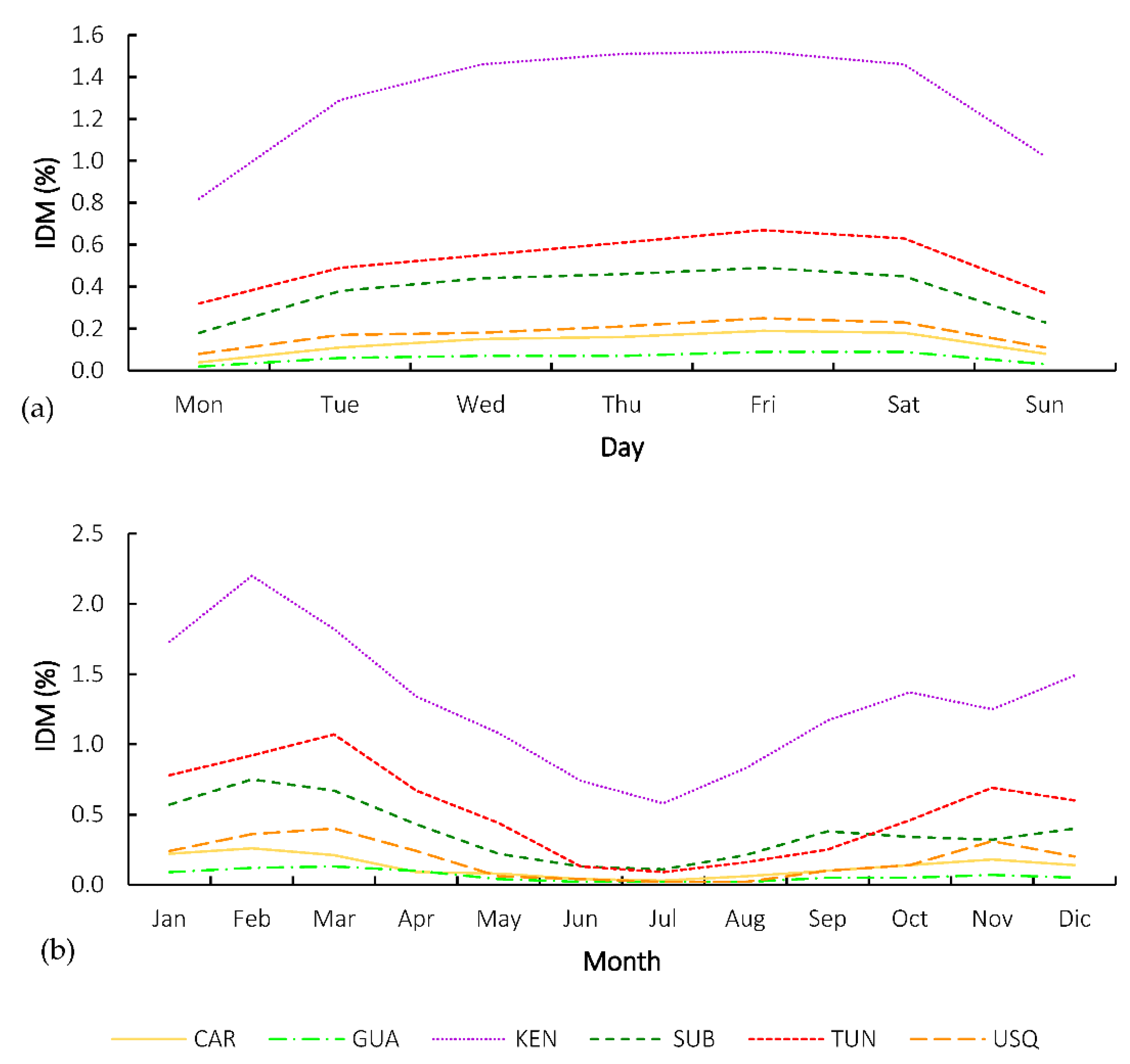
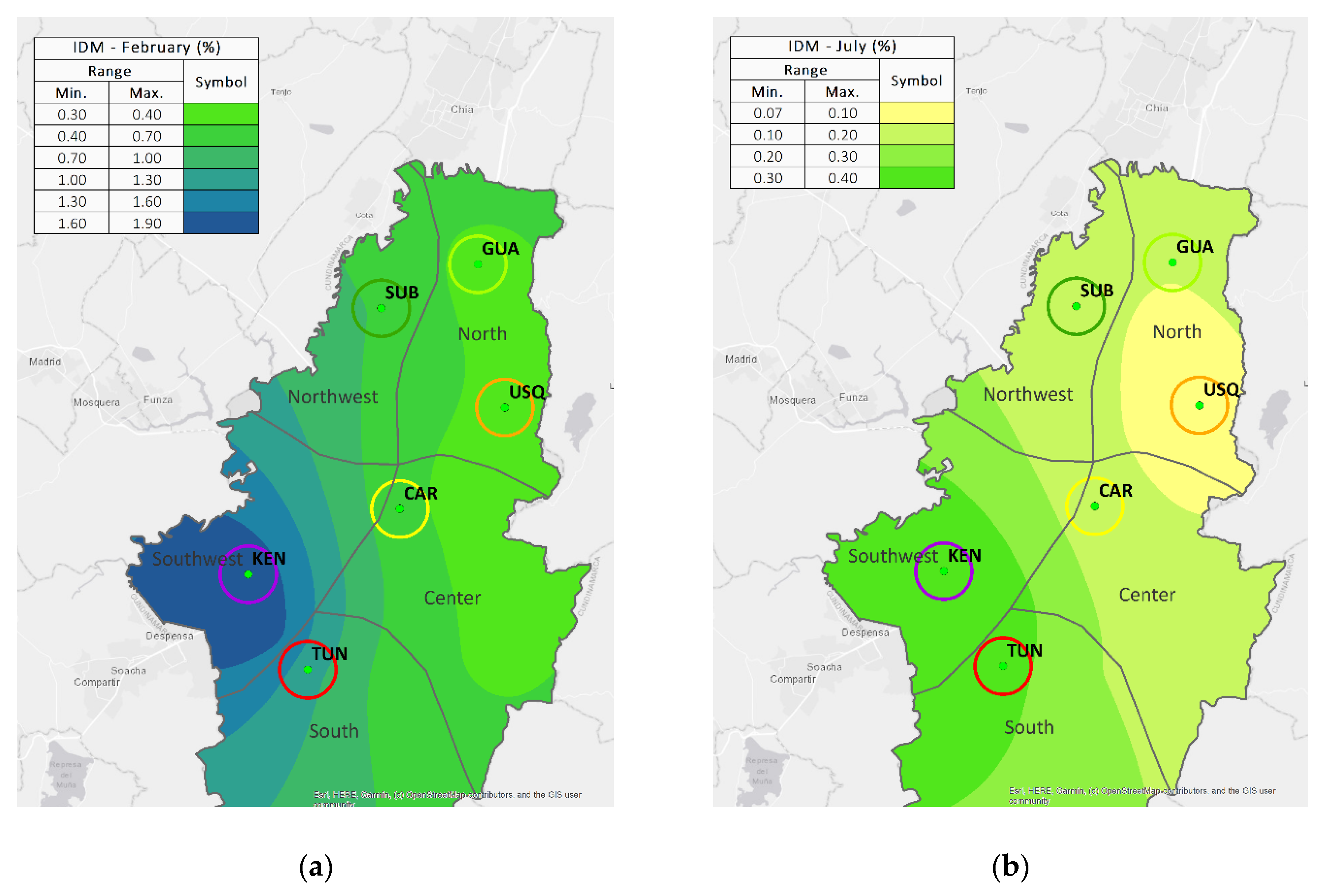
3.2. Spatiotemporal Variation of IDM

The IDM analysis for all ages and causes during the same day of PM10 exposure showed that the most critical interval was Wednesday to Saturday (average IDM = 0.505%; see Figure 5a). Indeed, this was possibly because the highest PM10 concentrations were observed from Wednesday to Saturday (Figure 2b). The least critical interval was from Sunday to Tuesday (average IDM = 0.322%). On average, the results suggested that during the most critical interval, the IDM was 1.57 times higher than it was in the least critical interval. The findings also hinted that during the most critical interval, it would be advisable to implement strategies that limit exposure to PM10, especially for the most vulnerable population (i.e., children, pregnant women, and the elderly), to reduce the negative impacts that PM10 generated on human health, mainly those people with respiratory and cardiovascular issues [47,48,49].
Considering the limit established by WHO for daily PM10, the results showed that during the entire study period (11 years), 37.9% of the time this limit was exceeded. For 4.17 years, the daily PM10 concentrations were greater than 50 μg/m3. On average, it was also detected by a linear regression model that for every 10% increase in exceeding the limit established by WHO, the IDM increased by 0.15% (y = 0.015x − 0.154; x = percentage of daily PM10 data > 50 μg/m3, and y = IDM in percentage; R2 = 0.972). For the monitoring station associated with the highest PM10 concentrations, a higher determination coefficient was evidenced in the linear regression model that was developed. At this monitoring station, for every 10% increase in exceeding limits, the IDM increased by 0.315% (y = 0.032x − 1.13; R2 = 0.981). In relation to PM and its effects on global human health, for example, it has been estimated that the loads attributable to PM2.5 pollution for ischemic heart disease, cardiovascular disease, lung cancer, lower respiratory tract infection, and mortality from chronic obstructive pulmonary disease were 17.1%, 14.2%, 16.5%, 24.7%, and 27.1%, respectively [47].
Monthly, IDM for all causes and ages showed, on average, the highest values during the interval from January to March (0.697%). Indeed, this monthly interval was the most critical in relation to observed PM10 concentrations (Figure 2c). In contrast, the interval from June to August was the least critical in relation to IDM (0.181%). These results were consistent with that reported by the District Environment Secretary of Bogotá D.C., which confirmed, that during 2018, 57% of acute respiratory infection (ARI) deaths in children under 5 years of age occurred during the first semester [23]. Indeed, the largest number of cases possibly occurred between January and March (the most critical interval). During 2011 and 2014, it was also observed that the highest number of people treated for ARI occurred during the first five months of the year. Subsequently, this number of visits decreased, as did PM10 concentrations [50]. The results suggested that the increase in these cases was related to the increase in IDM during the most critical interval, which was 3.86 times higher than the IDM during the least critical interval.
The findings showed that climatic variables possibly influenced the observed PM10 concentrations and, consequently, the temporal behavior of IDM. On average, the most critical month was February (IDM = 0.768%), and during this month thermal inversion phenomena were observed more frequently in Bogotá D.C., [50]. This relationship was also studied by Trinh et al. [51], who reported a direct correlation between the frequency of thermal inversions and the number of cases treated in hospitals for respiratory (r = 0.452; p-value < 0.05) and cardiovascular (r = 0.798; p-value < 0.05) diseases. These two types of diseases were commonly associated with urban air pollution. The results also suggested that the average IDM during the most critical month (February) was 5.42 times higher than the average IDM during the least critical month (July, average IDM = 0.142%; Figure 5b). This analysis was performed with respect to the same day of exposure (delay = 0 days).
The spatial behavior of IDM in the megacity during the most critical month (February) and the least critical month (July) was characterized by lower values in the eastern zone, which were increasing toward the western zone and reached the highest values in the southwestern zone (Figure 6). Thus, the areas of the megacity were classified as follows, according to the values of IDM: (i) low IDM = northern zone (0.105% in July and 0.403% in February), central zone (0.151% in July and 0.451% in February), and northwest zone (0.148% in July and 0.704% in February); (ii) medium IDM = southern zone (0.274% in July and 0.862% in February); (iii) high IDM = southwestern zone (0.336% in July and 1.42% in February). These results were consistent with the number of mortality cases from ARI in children under 5 years of age, as reported for 2018, where the highest number of cases was reported in the localities of Kennedy, Usme, and Ciudad Bolívar. This was in the southwest part of Bogotá D.C. [23]. Considering that the northern zone of the megacity was the one that showed the lowest IDM values and the southwestern zone showed the highest, it was detected that IDM in the southwestern zone was 3.36 times higher than IDM in the northern zone. Therefore, the results suggested a significant spatial variation in IDM in Bogotá D.C.

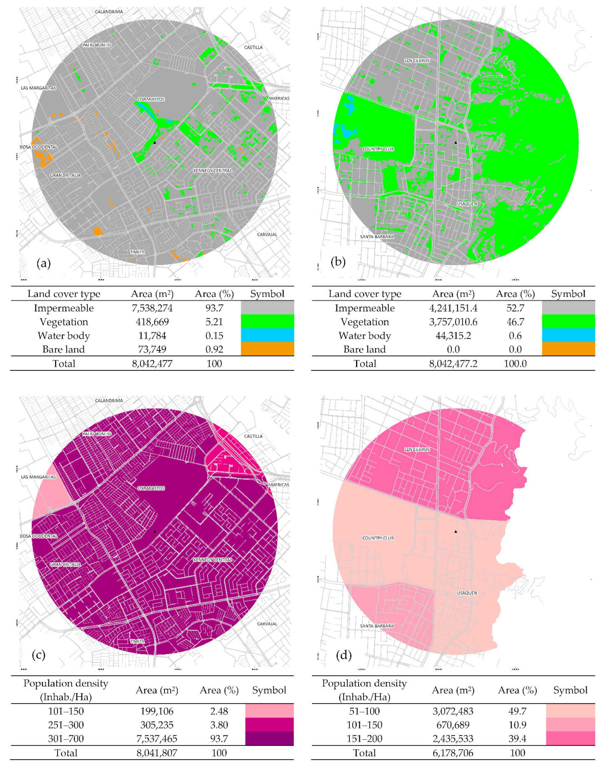
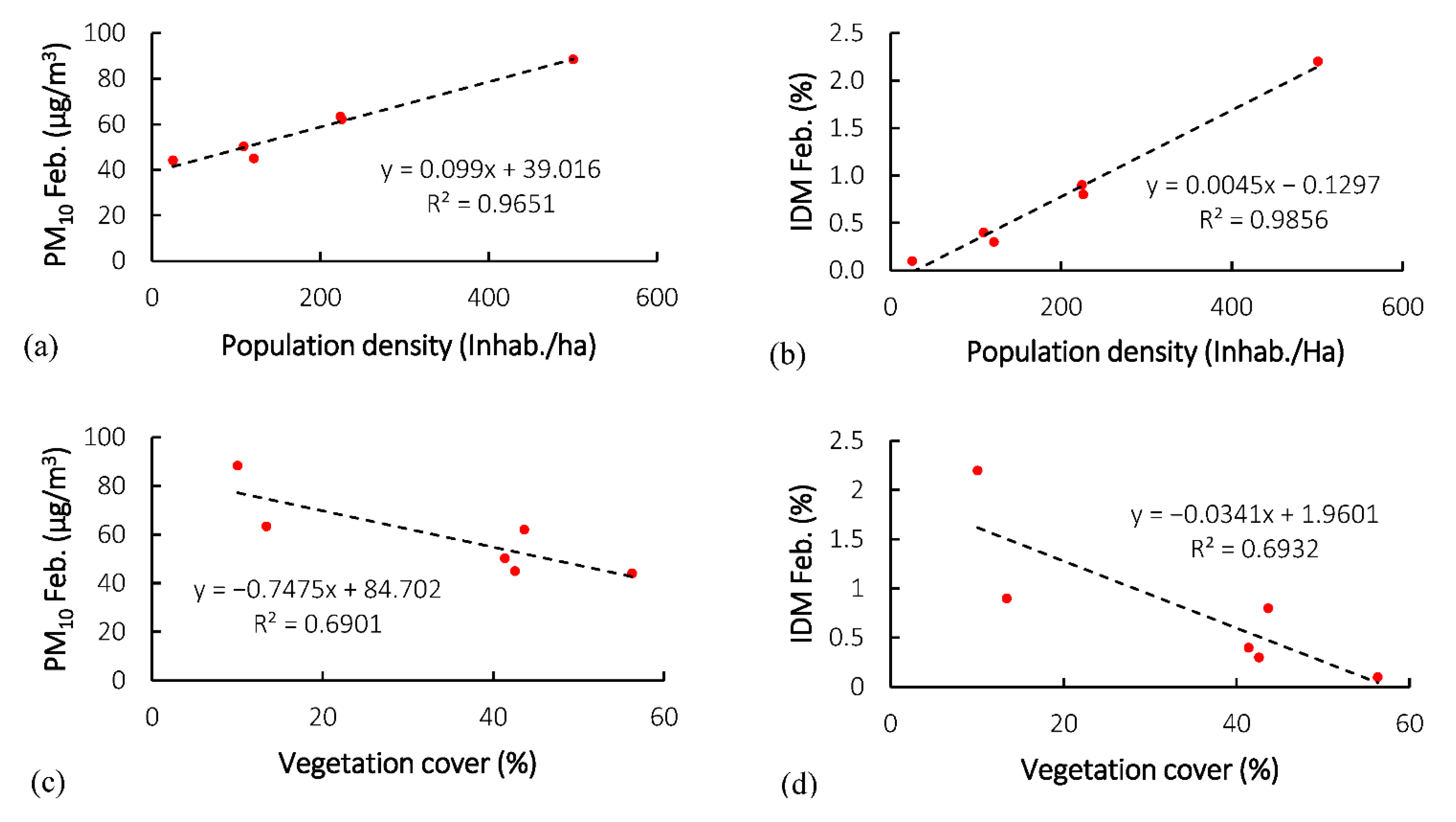
3.3. Relationship between Land Cover, PM10, and IDM

With respect to daily PM10 concentration levels, monitoring stations were classified according to their degree of air pollution as follows: (i) low pollution (GUA, USQ, and CAR), (ii) medium pollution (SUB and TUN), and high pollution (KEN). The results showed that the degree of pollution at each monitoring station was possibly associated with vegetation cover (radius of influence = 1600 m; Table 2). On average, the vegetation cover percentage observed at each monitoring station was as follows: GUA = 61.1%, USQ = 46.7%, SUB = 38.4%, CAR = 29.4%, TUN = 15.3%, and KEN = 5.21% (Figure 7a,b). Using linear regression models, the possible relationship between the vegetation cover percentage and the daily PM10 concentration during the most critical month (February) was analyzed. The IDM was also considered in this analysis. The findings showed that the relationships between the variables considered were better with an 800 m radius of influence rather than 1600 m. Thus, the results hinted that for every 10% increase in vegetation cover, the daily PM10 concentration tended to decrease by 7.5 μg/m3 (y = −0.74x + 84.7; x = vegetation cover in percentage, y = daily PM10 in μg/m3; R2 = 0.690; r = 0.831). In addition, IDM tended to decrease by 0.34% (y = −0.03x + 2.0; x = vegetation cover in percentage; y = IDM in percentage; R2 = 0.693; r = 0.832) (Figure 8a,b). Other studies also reported that with the increase in vegetation cover, there was a decrease in PM10 concentration [52]. Indeed, some studies reported that urban forests had positive effects on air quality and public health [53].
The results showed that when the radius of influence increased (between 800 and 1600 m), for the analysis of the different types of land cover, the tendency was for there to be a significant increase in impermeable cover in the established monitoring stations. Thus, the land covers of water bodies and bare land represented only between 0 % and 2.18% and 0 % and 9.83%, respectively (Table 2). This trend suggested an inverse relationship between vegetation and impermeable covers in Bogotá D.C. This behavior also confirmed the high urbanization in the megacity. In addition, the results showed that two of the monitoring stations were opposite in their vegetation cover percentage (radius = 1600 m). The vegetation cover percentage at the USQ station was 46.7% and at the KEN station, it was 5.21% (Figure 7a,b). This difference in vegetation cover also confirmed changes in the degree of PM10 pollution and IDM. The KEN station had 8.96 times less vegetation cover than the USQ station, which made its daily PM10 concentrations and IDM 1.56 and 4.80 times higher, respectively. Therefore, the results suggested that elevated values of impermeable land cover (KEN = 93.7%) were associated with high PM10 concentrations and, consequently, with high IDM values. Salata et al. [54] reported that on impermeable surfaces, there was a rebound phenomenon (resuspension) of PM, which significantly increased air pollution in urban areas. Conversely, an adsorption phenomenon was reported on vegetated surfaces, where vegetation acted as a pollution sink by intercepting and facilitating the PM10 deposition on it [55,56].
Additionally, the results showed that the KEN station was associated with a population density between 301 inhabitants and 700 inhabitants per hectare (impermeable cover area = 93.7%; radius = 1600 m; see Figure 7c). In contrast, the USQ station was associated in 49.7% and 39.4% of its area, respectively, with a population density between 51 to 100 and 151 to 200 inhabitants per hectare, respectively (vegetation cover area = 46.7%; radius = 1600 m; see Figure 7d). Indeed, impervious coverage was directly associated with population density. The findings suggested that the higher the population density in the megacity, the higher the daily PM10 concentration and, consequently, the higher the IDM. To study the association between these variables, linear regression models were developed for each of the radii of influence considered in this study (between 50–1600 m) and for the most critical month (February). The results indicated that the best fit in the models was observed for an 800 m radius of influence (R2 > 0.690; Figure 8). Moreover, it was observed that, on average, for each increase of 100 inhabitants per hectare in population density, daily PM10 concentrations tended to increase by 9.99 μg/m3 (y = 0.099x + 39; x = population density in inhabitants/ha, y = daily PM10 in μg/m3; R2 = 0.965; see Figure 8a). In addition, IDM increased by 0.45% (y = 0.005x − 0.13; x = population density in inhabitants/ha, y = IDM in percentage; R2 = 0.986; Figure 8b). Therefore, the results hinted that the densification of the megacity involved the loss of vegetation cover and possibly contributed to the increase in daily PM10 concentrations (Figure 8c,d). In other words, it is necessary to address the air quality problem in Bogotá D.C. through the development of public health and environmental policies, considering the spatiotemporal variation of PM10 concentrations, land cover, and IDM.

4. Conclusions

The results of this study of the influence of PM10 on human mortality from the variation of land cover in a Latin American megacity allowed us to reach the following conclusions. The results suggest that maximum hourly PM10 concentrations (8:00 h, average = 67.8 μg/m3) are associated with the displacement of inhabitants from their workplaces. On average, it was observed that for every 100,000 trips, there was probably an increase of 4.0 μg/m3 in hourly PM10 concentration (delay = 2 h). The busiest time interval in the megacity was Wednesday through Saturday, and the stations KEN, SUB, and TUN tended to exceed WHO guidelines during this time interval. The most critical monthly interval in air pollution was from January to March (average PM10 = 57.7 μg/m3) and the least critical monthly interval was from June to August (average PM10 = 42.6 μg/m3). Indeed, during these monthly intervals, there was possibly a medium-to-strong negative correlation between PM10 concentration and wind speed (r = −0.667). Spatially, a sectorization in the air pollution degree of the megacity was possibly observed. The southwestern sector showed, on average, daily PM10 concentrations that were 1.36 times higher than those in the northern sector. In addition, IDM at all ages and causes during the same day of PM10 exposure suggested that the most critical weekly interval was Wednesday through Saturday (average IDM = 0.505%). This was consistent with the weekly interval that showed the highest daily PM10 concentrations. The most critical weekly interval showed an IDM 1.57 that was times higher than that of the least critical weekly interval (Sunday–Tuesday). Monthly, the most critical time interval was from January to March (average IDM = 0.697%). During this monthly interval, the highest number of morbidity and mortality cases from ARI were reported. The spatial behavior of IDM again suggested a sectorization of the megacity. Thus, the southwest sector, which has the highest risk of air pollution, showed an IDM of up to 1.42% during the study period. In this sector, 41.2% of the mortality cases due to ARI were reported.
Additionally, the findings suggested an association between PM10 concentration, IMD, and land cover. In other words, the results hinted that, on average, for every 10% increase in urban vegetation cover, the daily PM10 concentration and IDM decreased by 7.5 μg/m3 and 0.34%, respectively. In this study, it was evident that the monitoring station with the lowest vegetation cover (8.96 times less) showed increases of 1.56 times and 4.8 times in the daily PM10 concentration and IMD, respectively. This was compared to the monitoring station with the highest vegetation cover (46.7%). Moreover, for every increase of 100 inhabitants/ha in population density, the daily PM10 concentration and the IDM increased by 9.99 μg/m3 and 0.45%, respectively. Indeed, the population densification of the megacity possibly implied the loss of vegetation cover and contributed to the increases in PM10 and IMD. Therefore, it was essential to address the air pollution problem in Bogotá D.C. through the development of public health and environmental policies, considering the spatiotemporal variation of PM10 concentrations, land cover, and IDM.
Finally, the following future research lines are visualized: (1) including in the IMD analysis the influence of PM2.5. This was not possible in this study because in Bogotá D.C., this air pollutant only recently began to be monitored (short time series); (2) in simple linear regression models developed for IDM and PM10 concentrations, adding variables to improve fit. For example, it is necessary to analyze the inclusion of additional climate or anthropic (e.g., population density) variables in multiple regression models to improve their adjustment; (3) simulating future changes in land cover to analyze consequences on PM10 and PM2.5 concentrations and IDM.

Author Contributions

Conceptualization, L.M.O.-A. and C.A.Z.-M.; Methodology, L.M.O.-A. and C.A.Z.-M.; Software, L.M.O.-A.; Validation, L.M.O.-A. and C.A.Z.-M.; Formal analysis, L.M.O.-A., C.A.Z.-M. and H.A.R.-Q.; Investigation, L.M.O.-A.; Resources, L.M.O.-A. and H.A.R.-Q.; Data curation, C.A.Z.-M.; Writing—original draft, L.M.O.-A., C.A.Z.-M. and H.A.R.-Q.; Writing—review & editing, C.A.Z.-M. and H.A.R.-Q.; Visualization, L.M.O.-A. and C.A.Z.-M.; Supervision, C.A.Z.-M. and H.A.R.-Q.; Project administration, C.A.Z.-M. and H.A.R.-Q.; Funding acquisition, C.A.Z.-M. and H.A.R.-Q. All authors have read and agreed to the published version of the manuscript.

Funding

This research received no external funding.

Institutional Review Board Statement

Not applicable.

Informed Consent Statement

Not applicable.

Data Availability Statement

Not applicable.

Acknowledgments

The authors appreciate the academic support of the Universidad Distrital Francisco José de Caldas (Colombia) and of the GIIAUD research group.

Conflicts of Interest

The authors declare no conflict of interest.

References

  1. Karanasiou, A.; Alastuey, A.; Amato, F.; Renzi, M.; Stafoggia, M.; Tobias, A.; Reche, C.; Forastiere, F.; Gumy, S.; Mudu, P.; et al. Short-Term Health Effects from Outdoor Exposure to Biomass Burning Emissions: A Review. Sci. Total Environ. 2021, 781, 146739. [Google Scholar] [CrossRef] [PubMed]
  2. Sun, X.; Luo, X.-S.; Xu, J.; Zhao, Z.; Chen, Y.; Wu, L.; Chen, Q.; Zhang, D. Spatio-Temporal Variations and Factors of a Provincial PM2.5 Pollution in Eastern China during 2013–2017 by Geostatistics. Sci. Rep. 2019, 9, 3613. [Google Scholar] [CrossRef] [PubMed] [Green Version]
  3. Soto, D.F.P.; Mejía, C.A.Z.; Miranda, J.P.R. Evaluación de la calidad del aire mediante un laboratorio móvil: Puente Aranda (Bogotá D.C., Colombia). Rev. Fac. Ing. Univ. Antioq. 2014, 71, 153–166. [Google Scholar]
  4. Blanco-Becerra, L.C.; Miranda-Soberanis, V.; Hernández-Cadena, L.; Barraza-Villarreal, A.; Junger, W.; Hurtado-Díaz, M.; Romieu, I. Effect of Particulate Matter Less than 10µm (PM10) on Mortality in Bogota, Colombia: A Time-Series Analysis, 1998–2006. Salud Pública México 2014, 56, 363–370. [Google Scholar] [CrossRef] [PubMed] [Green Version]
  5. Whyand, T.; Hurst, J.R.; Beckles, M.; Caplin, M.E. Pollution and Respiratory Disease: Can Diet or Supplements Help? A Review. Respir. Res. 2018, 19, 79. [Google Scholar] [CrossRef] [PubMed] [Green Version]
  6. Ning, G.; Wang, S.; Ma, M.; Ni, C.; Shang, Z.; Wang, J.; Li, J. Characteristics of Air Pollution in Different Zones of Sichuan Basin, China. Sci. Total Environ. 2018, 612, 975–984. [Google Scholar] [CrossRef]
  7. Yang, W.; Jiang, X. Evaluating the Influence of Land Use and Land Cover Change on Fine Particulate Matter. Sci. Rep. 2021, 11, 17612. [Google Scholar] [CrossRef]
  8. Liang, L.; Gong, P. Urban and Air Pollution: A Multi-City Study of Long-Term Effects of Urban Landscape Patterns on Air Quality Trends. Sci. Rep. 2020, 10, 18618. [Google Scholar] [CrossRef]
  9. East, J.; Montealegre, J.S.; Pachon, J.E.; Garcia-Menendez, F. Air Quality Modeling to Inform Pollution Mitigation Strategies in a Latin American Megacity. Sci. Total Environ. 2021, 776, 145894. [Google Scholar] [CrossRef]
  10. Zafra, C.; Suárez, J.; Pachón, J.E. Public Health Considerations for PM10 in a High-Pollution Megacity: Influences of Atmospheric Condition and Land Coverage. Atmosphere 2021, 12, 118. [Google Scholar] [CrossRef]
  11. Santovito, A.; Gendusa, C.; Cervella, P.; Traversi, D. In Vitro Genomic Damage Induced by Urban Fine Particulate Matter on Human Lymphocytes. Sci. Rep. 2020, 10, 8853. [Google Scholar] [CrossRef] [PubMed]
  12. Liu, C.; Henderson, B.H.; Wang, D.; Yang, X.; Peng, Z.-R. A Land Use Regression Application into Assessing Spatial Variation of Intra-Urban Fine Particulate Matter (PM2.5) and Nitrogen Dioxide (NO2) Concentrations in City of Shanghai, China. Sci. Total Environ. 2016, 565, 607–615. [Google Scholar] [CrossRef] [PubMed]
  13. Yang, H.; Chen, W.; Liang, Z. Impact of Land Use on PM2.5 Pollution in a Representative City of Middle China. Int. J. Environ. Res. Public Health 2017, 14, 462. [Google Scholar] [CrossRef]
  14. Anenberg, S.C.; Achakulwisut, P.; Brauer, M.; Moran, D.; Apte, J.S.; Henze, D.K. Particulate Matter-Attributable Mortality and Relationships with Carbon Dioxide in 250 Urban Areas Worldwide. Sci. Rep. 2019, 9, 11552. [Google Scholar] [CrossRef] [PubMed] [Green Version]
  15. Manojkumar, N.; Srimuruganandam, B. Health Effects of Particulate Matter in Major Indian Cities. Int. J. Environ. Health Res. 2021, 31, 258–270. [Google Scholar] [CrossRef] [PubMed]
  16. Leikauf, G.D.; Kim, S.-H.; Jang, A.-S. Mechanisms of Ultrafine Particle-Induced Respiratory Health Effects. Exp. Mol. Med. 2020, 52, 329–337. [Google Scholar] [CrossRef] [PubMed]
  17. Guo, P.; Su, Y.; Wan, W.; Liu, W.; Zhang, H.; Sun, X.; Ouyang, Z.; Wang, X. Urban Plant Diversity in Relation to Land Use Types in Built-up Areas of Beijing. Chin. Geogr. Sci. 2018, 28, 100–110. [Google Scholar] [CrossRef] [Green Version]
  18. Rodríguez-Villamizar, L.A.; Rojas-Roa, N.Y.; Fernández-Niño, J.A. Short-Term Joint Effects of Ambient Air Pollutants on Emergency Department Visits for Respiratory and Circulatory Diseases in Colombia, 2011–2014. Environ. Pollut. 2019, 248, 380–387. [Google Scholar] [CrossRef]
  19. Franco, J.F.; Gidhagen, L.; Morales, R.; Behrentz, E. Towards a Better Understanding of Urban Air Quality Management Capabilities in Latin America. Environ. Sci. Policy 2019, 102, 43–53. [Google Scholar] [CrossRef]
  20. Aguiar-Gil, D.; Gómez-Peláez, L.M.; Álvarez-Jaramillo, T.; Correa-Ochoa, M.A.; Saldarriaga-Molina, J.C. Evaluating the Impact of PM2.5 Atmospheric Pollution on Population Mortality in an Urbanized Valley in the American Tropics. Atmos. Environ. 2020, 224, 117343. [Google Scholar] [CrossRef]
  21. Sefair, J.A.; Espinosa, M.; Behrentz, E.; Medaglia, A.L. Optimization Model for Urban Air Quality Policy Design: A Case Study in Latin America. Comput. Environ. Urban Syst. 2019, 78, 101385. [Google Scholar] [CrossRef]
  22. Mendieta, E. Medellín and Bogotá: The Global Cities of the Other Globalization. City 2011, 15, 167–180. [Google Scholar] [CrossRef]
  23. SDA Informe Anual calidad del aire Bogotá 2018 » Observatorio Ambiental de Bogotá. Available online: https://oab.ambientebogota.gov.co/?post_type=dlm_download&p=13003 (accessed on 28 October 2022).
  24. U.S. EPA Title 40 of the CFR—Protection of Environment. Available online: https://www.ecfr.gov/current/title-40 (accessed on 28 October 2022).
  25. World Health Organization. Occupational and Environmental Health Team Guías de Calidad del aire de la OMS Relativas al Material Particulado, el Ozono, el Dióxido de Nitrógeno y el Dióxido de Azufre: Actualización Mundial 2005; Organización Mundial de la Salud: Geneva, Switzerland, 2006. [Google Scholar]
  26. Shakya, A.K.; Ramola, A.; Kandwal, A.; Prakash, R. Comparison of Supervised Classification Techniques with Alos Palsar Sensor for Roorkee Region of Uttarakhand, India. ISPRS-Int. Arch. Photogramm. Remote Sens. Spat. Inf. Sci. 2018, 425, 693–701. [Google Scholar] [CrossRef] [Green Version]
  27. Zafra, C.; Ángel, Y.; Torres, E. ARIMA Analysis of the Effect of Land Surface Coverage on PM10 Concentrations in a High-Altitude Megacity. Atmos. Pollut. Res. 2017, 8, 660–668. [Google Scholar] [CrossRef]
  28. DANE Proyecciones de Población. Available online: https://www.dane.gov.co/index.php/estadisticas-por-tema/demografia-y-poblacion/proyecciones-de-poblacion (accessed on 28 October 2022).
  29. MAVDT Manual de Operación de Sistemas de Vigilancia de la Calidad del Aire » Observatorio Ambiental de Bogotá. Available online: https://oab.ambientebogota.gov.co/?post_type=dlm_download&p=3768 (accessed on 28 October 2022).
  30. Berger, V.W.; Zhou, Y. Kolmogorov–Smirnov Test: Overview. In Wiley StatsRef: Statistics Reference Online; John Wiley & Sons, Ltd.: Hoboken, NJ, USA, 2014; ISBN 978-1-118-44511-2. [Google Scholar]
  31. Rebekić, A.; Lončarić, Z.; Petrović, S.; Marić, S. Pearson’s or Spearman’s correlation coefficient—Which one to use? Poljoprivreda 2015, 21, 47–54. [Google Scholar] [CrossRef]
  32. Conagin, A.; Barbin, D.; Demétrio, C.G.B. Modifications for the Tukey Test Procedure and Evaluation of the Power and Efficiency of Multiple Comparison Procedures. Sci. Agric. 2008, 65, 428–432. [Google Scholar] [CrossRef] [Green Version]
  33. Montealegre, B.J.E. Técnicas Estadísticas Aplicadas en el Manejo de Datos Hidrológicos y Meteorológicos; Instituto Colombiano de Hidrología, Meteorología y Adecuación de Tierras: Bogotá, Colombia, 1990. [Google Scholar]
  34. Carrera-Villacrés, D.V.; Guevara-García, P.V.; Tamayo-Bacacela, L.C.; Balarezo-Aguilar, A.L.; Narváez-Rivera, C.A.; Morocho-López, D.R. Relleno de Series Anuales de Datos Meteorológicos Mediante Métodos Estadísticos En La Zona Costera e Interandina Del Ecuador, y Cálculo de La Precipitación Media. Idesia 2016, 34, 81–90. [Google Scholar] [CrossRef] [Green Version]
  35. MADS Derecho Del Bienestar Familiar [RESOLUCION_MINAMBIENTEDS_2254_2017]. Available online: https://www.icbf.gov.co/cargues/avance/docs/resolucion_minambienteds_2254_2017.htm (accessed on 28 October 2022).
  36. Xu, T.; Liu, Y.; Tang, L.; Liu, C. Improvement of Kriging Interpolation with Learning Kernel in Environmental Variables Study. Int. J. Prod. Res. 2022, 60, 1284–1297. [Google Scholar] [CrossRef]
  37. Stafoggia, M.; Bellander, T.; Bucci, S.; Davoli, M.; de Hoogh, K.; de’ Donato, F.; Gariazzo, C.; Lyapustin, A.; Michelozzi, P.; Renzi, M.; et al. Estimation of Daily PM10 and PM2.5 Concentrations in Italy, 2013–2015, Using a Spatiotemporal Land-Use Random-Forest Model. Environ. Int. 2019, 124, 170–179. [Google Scholar] [CrossRef]
  38. Yuan, Z.; Yang, Y. Combining Linear Regression Models. J. Am. Stat. Assoc. 2005, 100, 1202–1214. [Google Scholar] [CrossRef]
  39. Franceschi, F.; Cobo, M.; Figueredo, M. Discovering Relationships and Forecasting PM10 and PM2.5 Concentrations in Bogotá, Colombia, Using Artificial Neural Networks, Principal Component Analysis, and k-Means Clustering. Atmos. Pollut. Res. 2018, 9, 912–922. [Google Scholar] [CrossRef]
  40. SDM Encuesta de Movilidad. Available online: https://www.movilidadbogota.gov.co/web/encuesta_de_movilidad (accessed on 28 October 2022).
  41. Ramírez, O.; Sánchez de la Campa, A.M.; Amato, F.; Catacolí, R.A.; Rojas, N.Y.; de la Rosa, J. Chemical Composition and Source Apportionment of PM10 at an Urban Background Site in a High–Altitude Latin American Megacity (Bogota, Colombia). Environ. Pollut. 2018, 233, 142–155. [Google Scholar] [CrossRef] [PubMed]
  42. MinTrabajo Leyes Desde 1992—Vigencia Expresa y Control de Constitucionalidad [CODIGO_SUSTANTIVO_TRABAJO]. Available online: http://www.secretariasenado.gov.co/senado/basedoc/codigo_sustantivo_trabajo.html (accessed on 28 October 2022).
  43. Martilli, A.; Sanchez, B.; Rasilla, D.; Pappaccogli, G.; Allende, F.; Martin, F.; Román-Cascón, C.; Yagüe, C.; Fernandez, F. Simulating the Meteorology during Persistent Wintertime Thermal Inversions over Urban Areas. The Case of Madrid. Atmos. Res. 2021, 263, 105789. [Google Scholar] [CrossRef]
  44. Gharibzadeh, M.; Saadat Abadi, A.R. Estimation of Surface Particulate Matter (PM2.5 and PM10) Mass Concentration by Multivariable Linear and Nonlinear Models Using Remote Sensing Data and Meteorological Variables over Ahvaz, Iran. Atmos. Environ. X 2022, 14, 100167. [Google Scholar] [CrossRef]
  45. Zhang, B.; Jiao, L.; Xu, G.; Zhao, S.; Tang, X.; Zhou, Y.; Gong, C. Influences of Wind and Precipitation on Different-Sized Particulate Matter Concentrations (PM2.5, PM10, PM2.5–10). Meteorol. Atmos. Phys. 2018, 130, 383–392. [Google Scholar] [CrossRef]
  46. Li, W.; Pei, L.; Li, A.; Luo, K.; Cao, Y.; Li, R.; Xu, Q. Spatial Variation in the Effects of Air Pollution on Cardiovascular Mortality in Beijing, China. Environ. Sci. Pollut. Res. Int. 2019, 26, 2501–2511. [Google Scholar] [CrossRef]
  47. Cohen, A.J.; Brauer, M.; Burnett, R.; Anderson, H.R.; Frostad, J.; Estep, K.; Balakrishnan, K.; Brunekreef, B.; Dandona, L.; Dandona, R.; et al. Estimates and 25-Year Trends of the Global Burden of Disease Attributable to Ambient Air Pollution: An Analysis of Data from the Global Burden of Diseases Study 2015. Lancet 2017, 389, 1907–1918. [Google Scholar] [CrossRef] [Green Version]
  48. Fazlzadeh, M.; Rostami, R.; Yousefian, F.; Yunesian, M.; Janjani, H. Long Term Exposure to Ambient Air Particulate Matter and Mortality Effects in Megacity of Tehran, Iran: 2012–2017. Particuology 2021, 58, 139–146. [Google Scholar] [CrossRef]
  49. Zhang, W.; Ma, R.; Wang, Y.; Jiang, N.; Zhang, Y.; Li, T. The Relationship between Particulate Matter and Lung Function of Children: A Systematic Review and Meta-Analysis. Environ. Pollut. 2022, 309, 119735. [Google Scholar] [CrossRef]
  50. IDEAM, Informes del Estado de la Calidad del Aire en Colombia. Available online: http://www.ideam.gov.co/web/contaminacion-y-calidad-ambiental/informes-del-estado-de-la-calidad-del-aire-en-colombia?p_p_id=110_INSTANCE_3uZc3mUViyRu&p_p_lifecycle=0&p_p_state=normal&p_p_mode=view&p_p_col_id=column-1&p_p_col_count=1&_110_INSTANCE_3uZc3mUViyRu_struts_action=%2Fdocument_library_display%2Fview_file_entry&_110_INSTANCE_3uZc3mUViyRu_fileEntryId=68521975 (accessed on 28 October 2022).
  51. Trinh, T.T.; Trinh, T.T.; Le, T.T.; Nguyen, T.D.H.; Tu, B.M. Temperature Inversion and Air Pollution Relationship, and Its Effects on Human Health in Hanoi City, Vietnam. Environ. Geochem Health 2019, 41, 929–937. [Google Scholar] [CrossRef]
  52. Gautam, S.; Brema, J. Spatio-Temporal Variation in the Concentration of Atmospheric Particulate Matter: A Study in Fourth Largest Urban Agglomeration in India. Environ. Technol. Innov. 2020, 17, 100546. [Google Scholar] [CrossRef]
  53. Xu, W.; Wu, Q.; Liu, X.; Tang, A.; Dore, A.J.; Heal, M.R. Characteristics of Ammonia, Acid Gases, and PM2.5 for Three Typical Land-Use Types in the North China Plain. Environ. Sci. Pollut. Res. 2016, 23, 1158–1172. [Google Scholar] [CrossRef] [PubMed] [Green Version]
  54. Salata, S.; Ronchi, S.; Arcidiacono, A. Mapping Air Filtering in Urban Areas. A Land Use Regression Model for Ecosystem Services Assessment in Planning. Ecosyst. Serv. 2017, 28, 341–350. [Google Scholar] [CrossRef]
  55. Riondato, E.; Pilla, F.; Sarkar Basu, A.; Basu, B. Investigating the Effect of Trees on Urban Quality in Dublin by Combining Air Monitoring with I-Tree Eco Model. Sustain. Cities Soc. 2020, 61, 102356. [Google Scholar] [CrossRef]
  56. Wu, J.; Wang, Y.; Qiu, S.; Peng, J. Using the Modified I-Tree Eco Model to Quantify Air Pollution Removal by Urban Vegetation. Sci. Total Environ. 2019, 688, 673–683. [Google Scholar] [CrossRef] [PubMed]
Figure 1. Location of the monitoring stations established in the study megacity (Google Earth Pro, https://earth.google.com/web/search/Bogot%C3%A1, accessed on 28 October 2018).
Atmosphere 13 01949 g001
Figure 2. Average PM10 concentrations under the (a) hourly, (b) daily, and (c) monthly time scales.
Atmosphere 13 01949 g002
Figure 3. Behavior of the hourly PM10 concentration in relation to the hourly amount of motor vehicle trips in Bogotá D.C.
Atmosphere 13 01949 g003
Figure 4. Average spatial variation of PM10 concentration in Bogotá D.C. during (a) the most critical month (February) and (b) the least critical month (July).
Atmosphere 13 01949 g004
Figure 5. Temporal variation of (a) daily and (b) monthly IDM in Bogotá D.C.
Atmosphere 13 01949 g005
Figure 6. Average spatial variation of IDM during (a) the most critical month (February) and (b) the least critical month (July), by PM10 concentrations.
Atmosphere 13 01949 g006
Figure 7. Variation of land cover and population density in the monitoring stations KEN (a,c) and USQ (b,d).
Atmosphere 13 01949 g007
Figure 8. Linear regression models (radius = 800 m) for the following relationships in February: (a) population density and PM10, (b) population density and IDM, (c) vegetation cover and PM10, and (d) vegetation cover and IDM.
Atmosphere 13 01949 g008
Table 1. Physical characteristics of the location areas of the established monitoring stations.
StationCARKENGUASUBTUNUSQ
Characteristics
Coordinates4°39′30.5″ N
74°5′2.28″ W
4°37′30.2″ N
74°9′40.8″ W
4°47′1.52″ N
74°2′39.1″ W
4°45′40.5″ N
74° 5′36.5″ W
4°34′34.4″ N
74°7′51.4″ W
4°42′37.3″ N
74°1′49.5″ W
Elevation (masl)257725802580257125892570
Annual mean PM10 (µg/m3)285028463839
Annual mean rainfall (mm)9321280796454544905
Hourly mean temperature (°C)S/R a15.214.514.4S/R aS/R a
Mean wind speed (m/s)1.192.301.001.391.191.60
LocalityBarrios UnidosKennedySubaSubaTunjuelitoUsaquén
Land classificationUrbanUrbanUrban/RuralUrban/RuralUrbanUrban/Rural
Urban land use bAUI/CS/D/I/R/SPAUI/CS/D/I/R/SPAAC/AUI/CS/D/I/R/SPAAC/AUI/CS/D/I/R/SPAUI/CS/D/I/R/SPAAC/AUI/CS/D/R/SP
Rural land use cN/AN/ASAP/ME/ACSAP/ME/ACN/ASAP/SE
Population density (inhabitants/ha)11226511511517382.2
Population/locality133,1261,019,7481,152,3871,152,387171,632535,693
Area/locality (ha)1189385510,04810,0489906514
Note: a S/R = no registration. b AAC = central activity area, AUI = integral urban area, CS = commerce and services, D = endowment, I = industrial, R = residential, and SP = protected land. c AC = high capacity, ME = special handling, N/A = not applicable, SAP = protected area system, and SE = expansion land.
Table 2. Types of land cover associated with each monitoring station.
StationRadius (m)Land Cover (%)
ImpermeableVegetationWater BodiesBare Land
2008 a2018200820182008201820082018
CAR80046.963.550.834.42.282.180.000.00
160063.374.134.724.12.001.760.000.00
KEN80087.390.59.610.40.580.602.480.49
160091.795.76.44.020.140.161.710.13
GUA80018.644.864.248.40.220.2016.96.70
160020.139.359.762.50.330.1319.98.97
SUB80046.148.746.141.10.100.327.659.83
160053.860.440.935.90.140.25.143.6
TUN80078.987.19.2717.530.000.0011.93.59
160080.383.312.717.90.040.206.922.73
USQ80061.455.838.644.20.000.000.000.00
160056.349.143.250.20.530.570.000.00
Note: a = year of study.
Publisher’s Note: MDPI stays neutral with regard to jurisdictional claims in published maps and institutional affiliations.

