Effects of Weather and Anthropogenic Precursors on Ground-Level Ozone Concentrations in Malaysian Cities

Abstract

Ground-level ozone (O₃) is a significant source of air pollution, mainly in most urban areas across the globe. Ground-level O₃ is not emitted directly into the atmosphere. It results from photo-chemical reactions between precursors and is influenced by weather factors such as temperature. This study investigated the spatial and temporal analysis of ground-level ozone and analyzed the significant anthropogenic precursors and the weather parameters associated with ground-level ozone during daytime and nighttime at three cities in peninsular Malaysia, namely, Kuala Terengganu, Perai, and Seremban from 2016 to 2020. Secondary data were acquired from the Department of Environment (DOE), Malaysia, including hourly data of O₃ with trace gases and weather parameters. The secondary data were analyzed using temporal analysis such as descriptive statistics, box plot, and diurnal plot as well as spatial analysis such as contour plot and wind rose diagram. Spearman correlation was used to identify the association of O₃ with its precursors and weather parameters. The results show that a higher concentration of O₃ during the weekend due to “ozone weekend effects” was pronounced, however, a slightly significant effect was observed in Perai. The two monsoonal seasons in Malaysia had a minimal effect on the study areas except for Kuala Terengganu due to the geographical location. The diurnal pattern of O₃ concentration indicates bimodal peaks of O₃ precursors during the peak traffic hours in the morning and evening with the highest intensity of O₃ precursors detected in Perai. Spearman correlation analysis determined that the variations in O₃ concentrations during day and nighttime generally coincide with the influence of nitrogen oxides (NO) and temperature. Lower NO concentration will increase the amount of O₃ concentration and an increasing amount of O₃ concentration is influenced by the higher temperature of its surroundings. Two predictive models, i.e., linear (multiple linear regression) and nonlinear models (artificial neural network) were developed and evaluated to predict the next day and nighttime O₃ levels. ANN resulted in better prediction for all areas with better prediction identified for daytime O₃ levels.

1. Introduction

Ground-level ozone (O₃) is one of the most common pollutants found in the Earth’s troposphere layers. It is therefore commonly referred to as a ‘bad’ ozone. The increased O₃ content in the Earth’s surface has consequences for human health, natural ecosystems, and vegetation development [1]. O₃ is primarily created by complex photochemical processes caused by anthropogenic precursors. A large percentage of ground-level ozone formation occurs in the presence of sunlight, typically the ultraviolet (UV) spectrum, when nitrogen oxides (NOx), carbon monoxide (CO), non-methane hydrocarbons (NmHCs), methane (CH₄), and volatile organic compounds (VOCs) react in the atmosphere. These are referred to as ozone precursors [2]. Ozone absorbs radiation and thus works as a powerful greenhouse gas. Despite rising temperatures, O₃ affects evaporation rates, cloud formation, precipitation amounts, and atmospheric circulation. These effects are most noticeable in areas where ozone precursors are emitted [3].

Ozone is an uncommon pollutant since it is not emitted directly into the environment. The transformation of land use from forest to agronomic, residential, and town creates a change, causing the O₃ precursor to rise, which can be seen clearly between urban and rural areas [4]. This process usually results in the development of large concentrations of O₃ downwind and in suburban regions resulting in higher anthropogenic precursors causing a high concentration of O₃ [5]. A greater source of ground-level ozone can be found in urban areas due to greater emissions from vehicles, power stations, industrial boilers, refineries, and chemical factories. The increasing population, industrial activities, and automobiles are the concrete reason for significantly increased emissions of VOCs and NO_x and, consequently, higher O₃ production can be expected in more populous areas.

In urban areas in particular, the concentration of NO released from traffic affects the formation of NO₂. During the day, sunlight plays an important role in starting reactions among O₃ precursors [4,6]. A high concentration of NO produced by motor vehicles may result in reduced O₃ concentration in busy areas, but it will increase the concentration of NO₂. High NO concentration will effective the titrate of atom (O) in urban areas due to emissions from the large amount of transportation activity. Through titration reactions with NO, O₃ is depleted, resulting in nitrogen dioxide (NO₂) and oxygen (O₂). The NO₂ produced can react along with O₃ to produce nitrate (NO₃) and O₂ [7]. On the contrary, at night there is no sunlight to react with precursors forming ozone. Thus, the presence of NO_x at night should have a significant decreasing impact on the concentrations of O₃ in an area. Many studies focus on the effect of ground-level ozone in the daytime rather than nighttime due to the significant relationship between O₃ with UVB. However, nighttime ozone is related to daytime ozone as the high preference may be carried over to the daytime. Likewise, the nighttime dispersion or accumulation of the precursors has a large impact on the ozone growth after sunrise. In addition, the overnight aloft ozone residual layer can play a role in morning time ozone rise [8].

In addition to O₃ precursors, meteorology plays a vigorous part in the atmospheric fate of ground-level O₃ in the lower boundary layer, including accumulation, dilution, and transport. Therefore, changes in meteorological conditions such as wind speed/direction, temperature, and relative humidity, can impact temporal variations of O₃ and anthropogenic precursors [9]. Correlation analysis is usually used to measure the relationship between the meteorological influences and parameters on tropospheric ozone [10,11]. Its positive or negative orientation provides a reliable reference for determining how specific climatic factors affect ozone concentrations. Temperature directly influences O₃ formation pathways by enhancing reaction rates of ozone precursors, ozone formation rates, and mechanism pathways [12]. On the one hand, high temperature is usually associated with sunshine duration, high solar irradiation, and low relative humidity that enhances ground-level ozone formation [13]. On the other hand, wind can significantly influence ground-level O₃ through dispersion and transportation [14]. The upwind and downwind geographical features affect O₃ levels at a site, hence, favorable wind conditions will help transport O₃ and its precursors downwind [10]. In general, wind speed negatively correlates with O₃ levels. Tong et al. [11] revealed that low wind speed (<4 ms⁻¹) enhanced O₃ accumulation. The boundary layer is stable at low wind, thus stabilizing O₃ levels. As for Malaysia, which has tropical weather with two distinct monsoonal seasons—the wet monsoon, i.e., northeast monsoon (NEM) from November to March and the dry monsoon, i.e., southwest monsoon (SWM) from June to September, with inter-monsoon seasons in between—the influence of O₃ levels on the seasonal monsoon are yet to be discovered [15].

The prediction of ozone levels using mathematical tools is very useful in providing early warnings to the population. Thus, statistical approaches have been widely used by researchers to study variations in O₃ concentrations with its precursors and weather parameters. Multiple linear regression (MLR) is one of the most common techniques used in the prediction of ground-level O₃ levels. MLR models a linear relationship between the independent and the dependent variables, thus the relationship of the O₃ level and other variables (including other air pollutants, its precursors, and meteorology parameters) can be determined [16]. Therefore, due to its simplicity and reliability, MLR has been successfully used as a predictive tool worldwide [17,18,19,20]. Besides providing a simple linear relationship of ozone concentration with its precursors and weather parameters, MLR may not deliver accurate forecasts in some complex situations such as non-linear data and extreme values data. Artificial neural networks (ANN), one of the most common machine learning techniques, can be a useful tool to extract information from non-linear data such as air quality and meteorology. Currently, the application of neural networks has become more popular for predicting ground-level O₃ concentrations. A lot of researchers have effectively adopted ANN as a predictive tool to model O₃ concentration [21,22,23,24,25] and its precursor, NO₂ [26]. Even though many studies have been carried out in the world investigating the association between the weather and ozone concentration using MLR and ANN, there is still a shortage of work, especially in Malaysia.

In this research, the main aim was to analyze the spatial and temporal variability of O₃ concentrations with its precursors and weather parameters during daytime and nighttime in selected urban areas in peninsular Malaysia. Studying the characteristics of O₃ concentrations especially in the rarely pronounced urban areas in peninsular Malaysia are helpful toward a better understanding of the variation in O₃. At the local level, the photochemical characteristics of O₃ vary with geographical location because the generation of O₃ is significantly affected by local environmental conditions, especially temperature, solar radiation, and atmospheric stagnation. In addition, two predictive models (i.e., linear and nonlinear models) were developed and attempted to forecast daytime and nighttime O₃ levels. Most of the O₃ level predictive models focused on daytime prediction, however, it is important to model the accumulation of O₃ at nighttime as some of the places are showing an increasing trend of O₃ during nighttime.

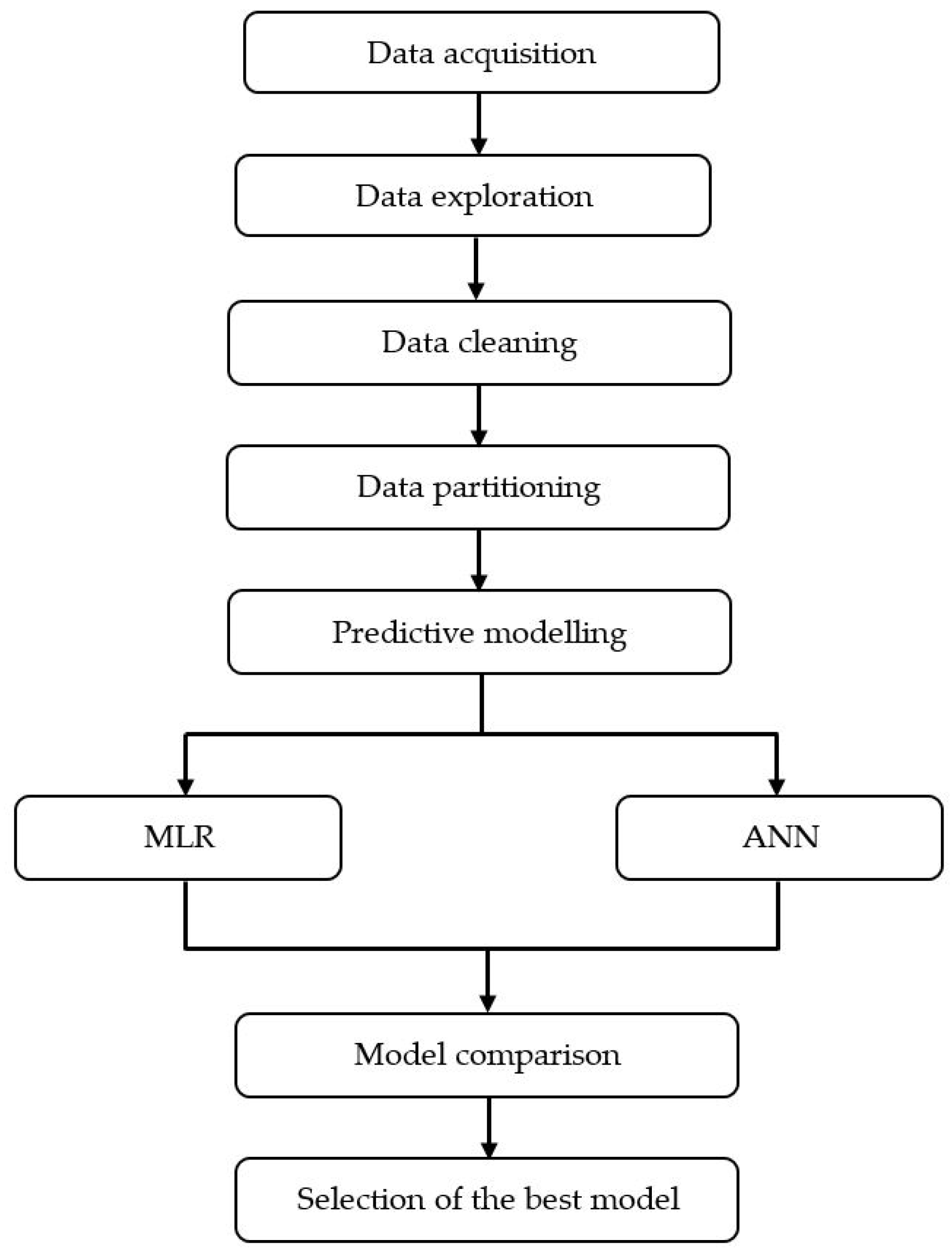
2. Materials and Methods

2.1. Air Pollutant Dataset

Continuous hourly air quality data from 2016 to 2020 were obtained from the Air Quality Division of the Department of Environment (DOE) Malaysia. This study used 12 variables that were divided into two groups. One group comprised seven air pollutants, such as O₃ (ppm), NO_x (ppm), NO (ppm), SO₂ (ppm), NO₂ (ppm), CO (ppm), and PM₁₀ (µg/m³). While weather parameters are wind speed (km/h), temperature (°C), humidity (%), UVB (W/m²), and wind direction (^o). These data were sorted in Microsoft Excel according to the diurnal cycle since the O₃ level significantly varies during daytime and nighttime. The diurnal cycle of daytime O₃ was from 7:00 am to 7:00 pm and the nighttime cycle was from 8:00 pm to 6:00 am. Malaysia experiences a slightly longer daytime period due to its location near the equator.

In this study, urban areas located in peninsular Malaysia, namely, Kuala Terengganu, Perai, and Seremban were chosen. According to Wan Mahiyuddin et al. [27], ground-level ozone exposure has reached levels that pose severe health hazards inside the larger Klang Valley sprawling city, which is Malaysia’s most densely populated area. However, there are very limited studies of O₃ variation reported in Kuala Terengganu, Seremban, and Perai. The details of the study areas are tabulated in

Table 1. Details of Study Areas.

Location	Station	Population [28]	Background of Study Areas
Kuala Terengganu	Sekolah Kebangsaan Pusat Chabang Tiga (5.3066, 103.1217)	261,300	Urban Residential areas
Seremban	Kolej Vokasional Ampangan (2.7250, 101.9708)	467,800	Urban Residential areas
Perai	Sekolah Kebangsaan Seberang Jaya 2 (5.3979, 100.4043)	630,999	Industrial areas Residential areas

.

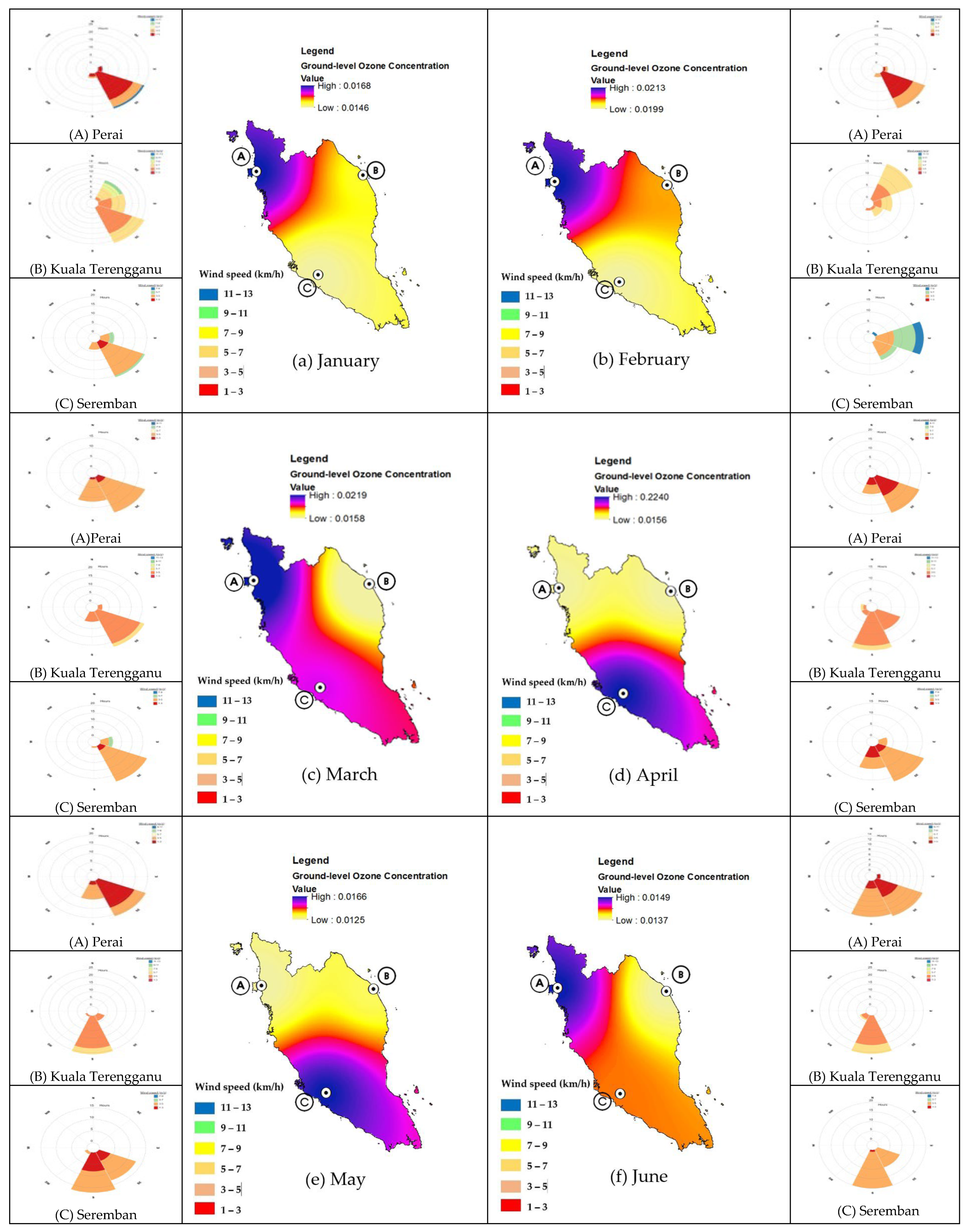
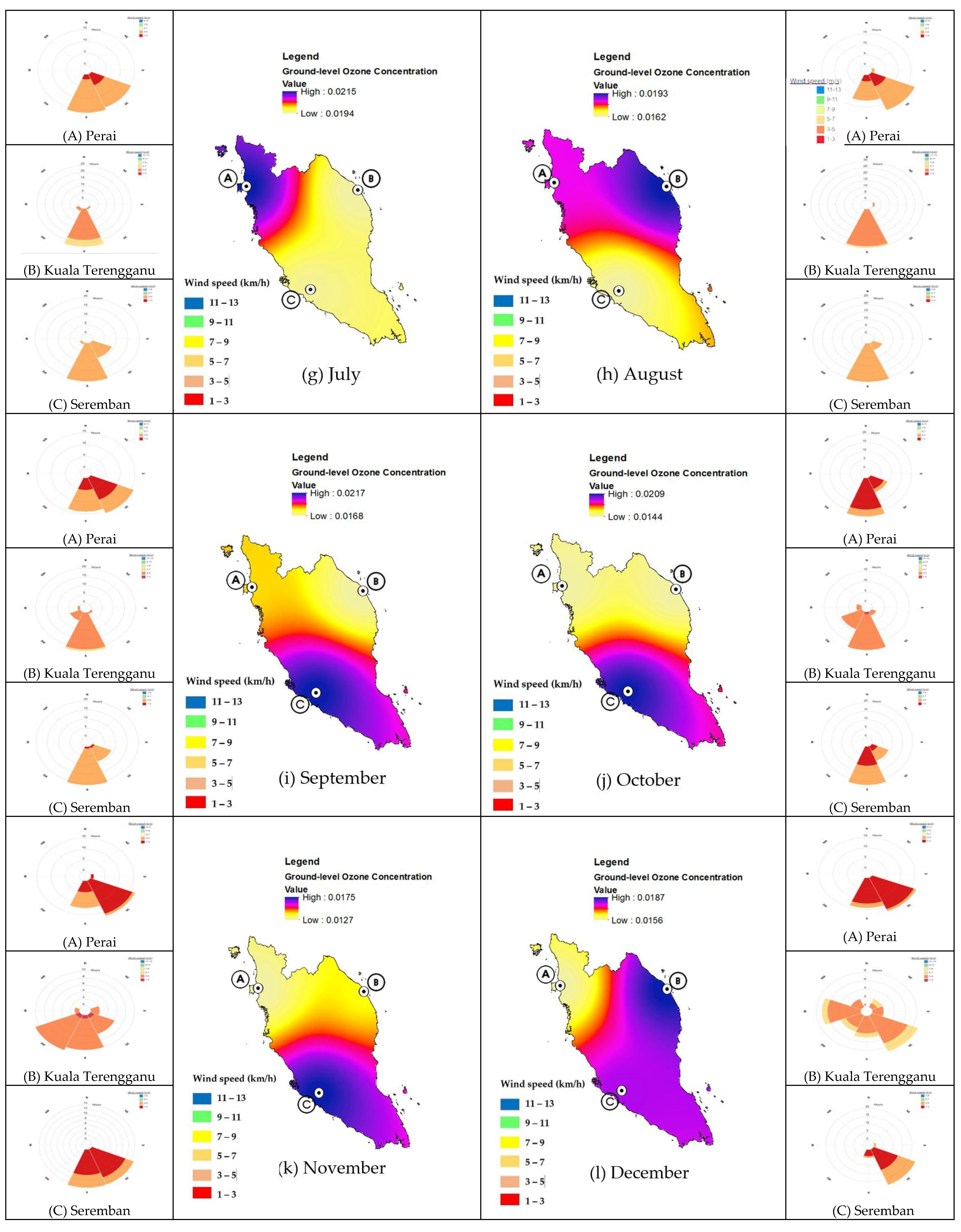
2.2. Spatial Analysis

In this study, two spatial analyses were conducted: contour plot and wind rose diagram. Contour plot was used to examine the monthly distribution of O₃ levels at a regional spatial scale. The spatial interpolation method can effectively estimate the pollutant concentration at any point within the regional ambient air range. Applying the first law of geography, the ordinary kriging method (OKM) was used to analyze the continuous distribution of the concentration of O₃ among the stations. A monthly wind rose diagram was generated using Microsoft Excel.

2.3. Measure of Association Using Spearman Correlation

In this research, Spearman Correlation was used to analyze the significant precursors and weather parameters toward O₃ concentration and the results are presented in the form of a heat matrix. A nonparametric measure of the relationship between the two sets of ordinal-ranked values is Spearman rank correlation (ρ) [29]. A Spearman coefficient is essentially a Pearson correlation coefficient calculated using the ranks of the values of the two variables rather than their actual values. The formula is shown below [30]:

$$\rho =1-\frac{6\sum d_i^2}{n\left(n^2-1\right)}$$

(1)

where ρ = Spearman’s Correlation coefficient; d_i = difference between two ranks of each observation; and n = number of observations.

The analysis was divided into two different time cycles: daytime and nighttime.

Table 2. Description of the correlation related to the value of ρ [31].

Value of ρ	Station
0.00–0.19	Very weak
0.20–0.39	Weak
0.40–0.59	Moderate
0.60–0.79	Strong
0.80–1.00	Very strong

shows the description of the correlation using the following guide for the absolute value of “ρ”:

2.4. Prediction Model

In this study, the daytime and nighttime O₃ levels for the next day (the next 24 h) are predicted. As shown in Figure 1, data acquisition, exploration, cleaning, and partitioning are part of the data preparation. The data acquisition describes the information of data and parameters included in this study (as presented in Section 2.1). Secondly, a descriptive analysis including central tendency (mean and median) and dispersion (standard deviation) analyses were measured in data exploration. Next, data cleaning explained the technique involved in imputing the missing observation. In this study, expectation maximization (EM) was used to fill in the missing data as this method was reported as the most reliable method in estimating missing air pollutant observation data [32]. Before developing the model, the original dataset was partitioned into two datasets for training and validation. Out of the total data, 80% were used to develop the model, whereas the rest of the data were used to validate the model. Parameters that had moderate to strong correlation (ρ ≥ 0.4) with the O₃ level from Spearman correlation analysis were used as the inputs for the prediction models. The details of predictive models are discussed in Section 2.4.1 and Section 2.4.2 and the performance evaluation for comparing the performances of the model is explained in Section 2.4.3.

2.4.1. Multiple Linear Regression (MLR)

MLR is a conventional method used to model air pollutants. MLR models the connection between two or more independent variables and a dependent variable by fitting a linear equation to the observed data. Multiple linear regression analysis is a statistical technique that can be used to examine the relationship between a single dependent (criterion) variable, Y, and several independent (predictor) variables, Xs. A random response Y relates to a set of independent variables X1, X2, …, X_i based on the multiple regression model. The equation can be read as [33]:

Y_i = β₀ + β₁·X₁ + … + β_k·X_i + ϵ_i

(2)

where, i is equal to n observations; Y_i = dependent variable (daytime and nighttime O₃ levels); X_i is the explanatory variables (ozone precursors and weather parameters); Β₀ is the y-intercept (constant term); Β_k is the slope coefficients for each explanatory variable; and ϵ = the model’s error term (also known as the residuals).

2.4.2. Artificial Neural Network (ANN)

A feed-forward backpropagation neural network (FFBP) was used in this study. The structure of FFBP was composed of three layers of neurons called the input, hidden, and output layers. The first layer of neurons consisted of an input layer, representing independent variables. The second layer was the hidden layer, which is responsible for processing the input weight from the input layer and transferring it to the output layer. The third layer was the output layer, which represents the next-day prediction of daytime and nighttime O₃ levels. The operation was conducted using the usual sigmoid function as the activation function.

2.4.3. Performance Indicators

Performance indicators are used to evaluate the predictive model by MLR and ANN. It was used to assess the model’s applicability in predicting daytime and nighttime O₃ concentrations. The performance measures applied in this study are mean absolute error (MAE), root mean squared error (RMSE), and correlation (r) Table 3 [34].

Table 3. Performance indicators.

Performance Indicators	Equation	Better Predictability if
Mean Absolute Error	$MAE=\frac{{{\displaystyle \sum }}_{i=1}^n\left|P_{i-}{O}_i\right|}{n}$	Closer to 0
Root Mean Squared Error	$RMSE=\frac{1}{n-1}{\displaystyle \sum _{i=1}^n}{(P_i-O_i)}^2$
Correlation	$r=\frac{{{\displaystyle \sum }}_{i=1}^n\left(P_i-\overline{P}\right)\left(O_i-\overline{O}\right)}{\left(n-1\right)\left(S_p\right)\left(S_o\right)}$	Closer to −1 or +1

Table 3. Performance indicators.

Performance Indicators	Equation	Better Predictability if
Mean Absolute Error	$MAE=\frac{{{\displaystyle \sum }}_{i=1}^n\left|P_{i-}{O}_i\right|}{n}$	Closer to 0
Root Mean Squared Error	$RMSE=\frac{1}{n-1}{\displaystyle \sum _{i=1}^n}{(P_i-O_i)}^2$
Correlation	$r=\frac{{{\displaystyle \sum }}_{i=1}^n\left(P_i-\overline{P}\right)\left(O_i-\overline{O}\right)}{\left(n-1\right)\left(S_p\right)\left(S_o\right)}$	Closer to −1 or +1

where;

n	=	total number of hourly measurements at a particular site;
$P_i$	=	predicted values of a single set of hourly monitoring data;
$O_i$	=	the observed values from a single set of hourly monitoring records;
$\overline{P}$	=	the mean of the predicted values from a single set of hourly monitoring data;
$\overline{O }$	=	the mean of the observed values from a single set of hourly monitoring data;
$S_p$	=	the standard deviation of the predicted values from a single set of hourly monitoring data;
$S_o$	=	the standard deviation of the observed values from a single set of hourly monitoring data.

3. Results and Discussion

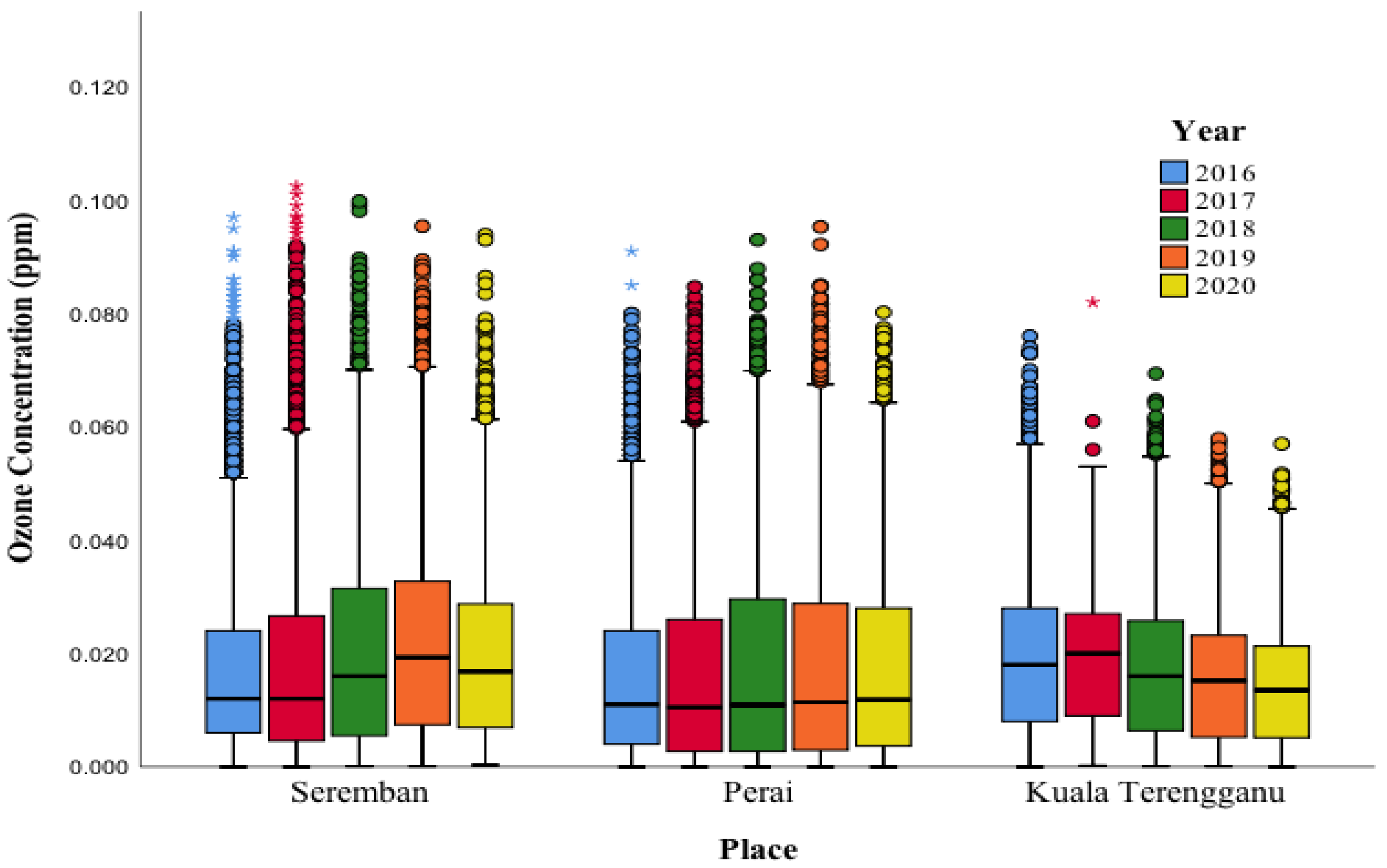
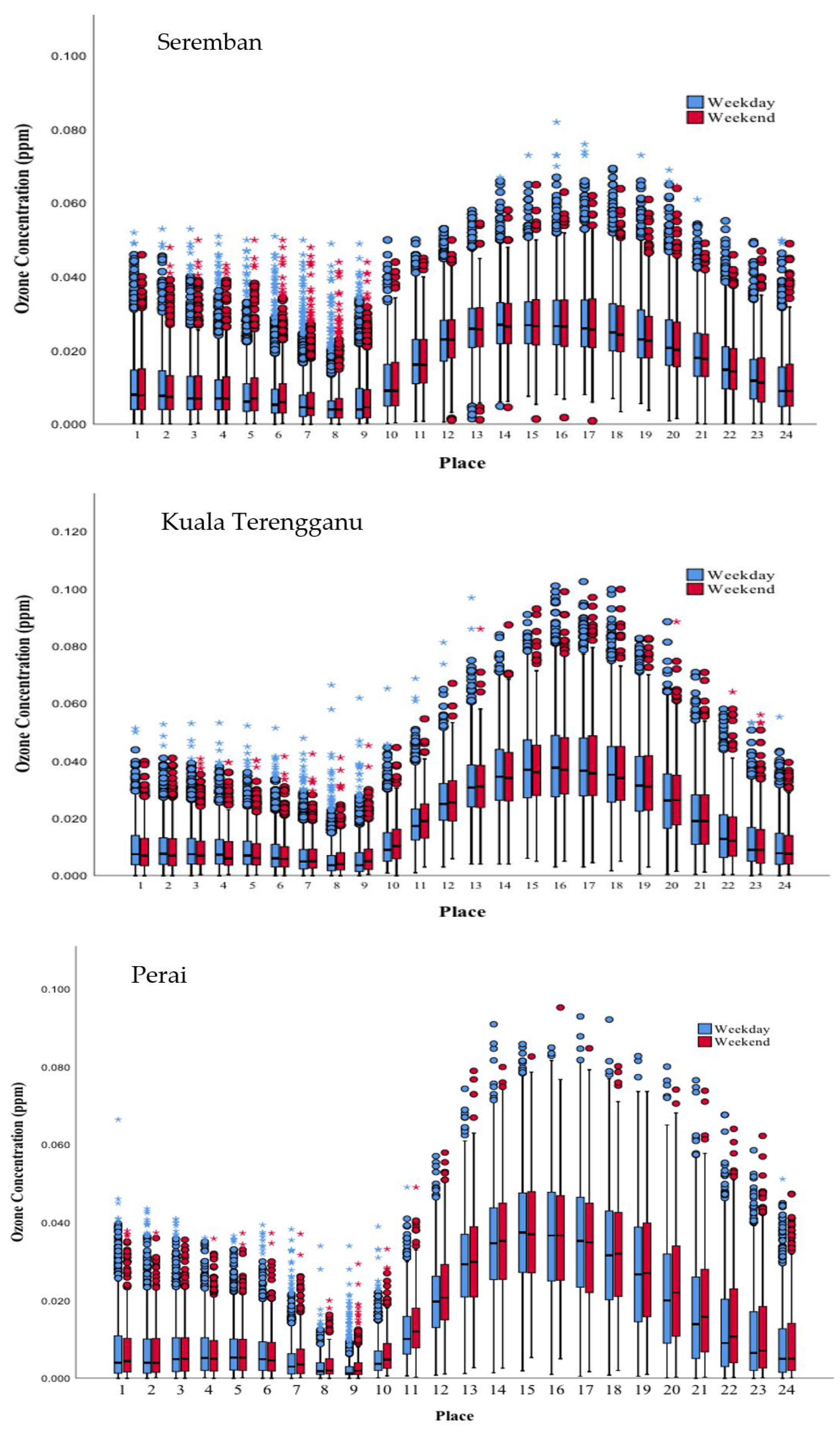
3.1. Spatiotemporal Variation of Ground-Level Ozone

Table 4. Descriptive statistic of ground-level ozone concentration in Perai, Seremban, and Kuala Terengganu from 2016 to 2020.

Study Area	Year		2016	2017	2018	2019	2020
Perai	N	Valid	8237	5513	8260	8350	8292
		Missing	547	1303	500	410	492
	Mean		0.01543	0.01629	0.01749	0.01757	0.01718
	Median		0.01100	0.01050	0.01140	0.01090	0.01185
	Std. Deviation		0.014710	0.16441	0.017208	0.017544	0.015890
	Minimum		0.000	0.000	0.000	0.000	0.000
	Maximum		0.091	0.085	0.095	0.093	0.080
Seremban	N	Valid	6478	5886	8327	8356	8373
		Missing	2306	928	426	406	409
	Mean		0.01686	0.01748	0.02030	0.02194	0.01943
	Median		0.01200	0.01200	0.01600	0.01930	0.01680
	Std. Deviation		0.014792	0.016436	0.017167	0.016930	0.014807
	Minimum		0.000	0.000	0.000	0.000	0.000
	Maximum		0.097	0.103	0.100	0.095	0.094
Kuala Terengganu	N	Valid	8335	5975	8215	8320	8337
		Missing	449	836	558	440	447
	Mean		0.01981	0.01776	0.01739	0.01559	0.01412
	Median		0.01800	0.01670	0.01600	0.01520	0.01350
	Std. Deviation		0.013018	0.012303	0.012521	0.011184	0.009916
	Minimum		0.000	0.000	0.000	0.000	0.000
	Maximum		0.076	0.082	0.069	0.058	0.057

represents a data summary for ground-level ozone measurement in the three study areas for the period of 5 years. Overall, the mean concentration of ozone levels for Perai, Kuala Terengganu, and Seremban is below the limit (0.1 ppm) as postulated in the Malaysia Ambient Air Quality Standard (MAAQS). The maximum O₃ level in 2018 was recorded as the highest value compared with all study areas during the five year period. The highest ozone concentration reading in Perai was 0.095 ppm in 2018 with a mean of 0.0175 ppm while the lowest maximum value was 0.080 ppm in 2020 with a mean value of 0.01718 ppm. From the mean concentration, Perai and Seremban showed an incremental trend from 2015 to 2019 whereas Kuala Terengganu showed a decremental trend of O₃ levels. As a result, the smallest range of data was observed, i.e., 0 ppm to 0.009 ppm. Seremban recorded the highest concentration of O₃ starting from 2018 with a mean value of 0.022 ppm. Lower concentrations were recorded in Kuala Terengganu and the lowest was in Perai. The standard deviation indicates that the O₃ measurement records showed less variables and a smaller range of O₃ levels was observed in Kuala Terengganu.

Figure 2 represents the box plot of hourly O₃ concentrations in Seremban, Perai, and Terengganu from 2016 to 2020. The O₃ levels in Seremban and Perai were observed to have higher variability in 2018 and 2019. Seremban had the maximum O₃ level of 0.103 ppm in 2019 and recorded the lowest maximum concentration in 2020 with the value of 0.094 ppm. The highest concentration in Perai was 0.095 ppm in 2018 while the concentration decreased in 2019 and 2020 with maximum values of 0.093 ppm and 0.80 ppm, respectively. The data distribution for all years at Perai were skewed to the right which indicates a positive skew. Conversely, the concentration of O₃ at Kuala Terengganu was the lowest compared with Perai and Seremban. The maximum O₃ concentration was 0.082 ppm in 2017 while the lowest was 0.057 ppm in 2020 as illustrated in Figure 2. Kuala Terengganu experienced a decrease in O₃ concentration values by year starting from 2016 to 2020. It was observed that O₃ levels in Kuala Terengganu were less variable compared with Seremban and Perai.

Overall, the distribution of O₃ levels in all study areas were skewed to the right which indicates that extreme concentration occurred. Seremban was observed to have a high exceedance of O₃ levels especially in 2017. The monitoring station observed a decrease in 2020 due to less transportation use and factory shutdowns because of epidemic transmission of COVID-19. Malaysia’s response to the COVID-19 pandemic resulted in unprecedented reductions in economic activity in 2019 to 2021. After accounting for weather changes, lockdown events lowered population-weighted concentrations of NO₂ and particulate matter by around 60% and 31%, respectively, as well as O₃ concentrations [32]. Reductions in transportation sector emissions are largely responsible for the NO₂ variances. The different results in three monitoring stations are believed to be influenced by variations in temperature, humidity, and wind speed.

Monthly variations of tO₃ levels for the three study areas can be analyzed using contour plots and a wind rose diagram as depicted in Figure 3. During the early months of the year, Perai recorded the highest concentrations compared with Seremban and Kuala Terengganu with mean O₃ concentrations of 0.0168 ppm in January, 0.0213 ppm in February, and 0.0219 ppm in March. Perai experienced very light wind (1 km/h to 3 km/h) in January and February that came from the southeast and light wind (3 km/h to 5 km/h) in March from the southeast and south. Latif et al. [6] reported that the northern area of Peninsular Malaysia experienced a hot and dry wind from the northeast, especially from Indochina and the South China Sea to the north of peninsular Malaysia. Nonetheless, the wind rose diagram indicates that Perai did not receive any wind from the northeast direction; hence, the high O₃ levels during this month were most probably due to the low speed of wind. On the other hand, Seremban was observed to experience the highest concentrations of O₃ levels during the inter-monsoon (April) with the value of 0.0224 ppm. During this month, Seremban mostly received light wind (3 km/h to 5 km/h).

Perai once again recorded the highest levels of O₃ compared with other areas during the early dry monsoon (June and July), which is the southwest monsoon, while Seremban recorded high O₃ levels at the end of the summer monsoon (September) and during inter-monsoon (October and November). Weak wind (1 km/h to 5 km/h) was detected during the early season of the dry monsoon in Perai which might have influenced the dispersion of pollutants [10]. A gentle breeze (12 km/h to 19 km/h) is at least required to impact the greater dispersion of air pollutants, resulting in lower air pollution concentrations in areas with stronger winds. A similar situation can be observed in Seremban where very light wind (1 km/h to 3 km/h) was detected especially from October to December resulting in almost stagnant air in the inland areas.

In the other hand, O₃ levels in Kuala Terengganu were detected to be higher at the end of the dry monsoon, i.e., in September and October. Light air (3 km/h to 5 km/h) from the south and southwest was detected in Kuala Terengganu during this time, hence confirming the influence of the southwest monsoon on O₃ levels at this area.

Overall, higher O₃ levels at all areas can be observed from June to October, i.e., during the southwest monsoon (dry monsoon). However, only Kuala Terengganu shows the influence of the monsoon in contributing to higher O₃ levels in that area. Other areas, i.e., Perai and Seremban received light wind (1 km/h to 5 km/h) from the south and southeast. However, during this hot and dry climate, a low amount of precipitation and lower wind speed can be expected, hence it might influence the formation of ozone via complex photochemical reactions with other pollutants in the atmosphere that remain longer in the atmosphere due to poor dispersion [35].

Figure 4 shows weekly variations of O₃ levels in Seremban, Kuala Terengganu, and Perai. Generally, the same diurnal trend of O₃ variations were observed for the three monitored areas. On a weekly basis, the weekend and weekdays exhibited higher O₃ levels starting from 10:00 am until 5:00 pm, whereas the O₃ levels started to decrease starting at 6:00 pm until the next-day morning at around 9:00 am. The lowest O₃ level was detected in Perai at 8:00 am during the weekday compared with other places, while the highest O₃ concentration was found in Seremban at 5:00 pm during the weekdays.

Seremban showed a higher distribution of O₃ levels during weekdays compared with the weekend. Extreme concentrations of O₃ levels were observed early in the morning (from 1:00 am to 9:00 am) and in the evening (3:00 pm to 6:00 pm). During nighttime, the absence of UV light reduced the O₃ photochemical reaction rate and the O₃ concentrations because of continuous chemical degradation by NO and titration [36].

In Kuala Terengganu, a higher variability of O₃ concentration was monitored during weekdays compared with the weekend. However, during the weekend, a higher concentration of O₃ was detected in the morning (from 8:00 am to 12:00 pm) and the concentration was slightly low during the peak wavelength of solar radiation (from 2:00 pm to 4:00 pm) if compared with the variation during weekdays. However, the O₃ level increased again from 5:00 pm onwards compared with the weekday variations. Similar O₃ variations can be found in Perai with a higher degree of difference in O₃ between the weekend and weekdays, especially in Perai because the monitoring areas are located next to the main highway of the South–North and Butterworth–Kulim Express Highway, which results in higher concentrations of O₃ during the weekend because many people use the highway to travel to their hometowns on weekends.

Higher O₃ levels during the weekend compared with weekdays may be caused by the differences in the number of vehicles. A high level of ozone on the weekend is a well-known phenomenon known as the “ozone weekend effect” (OWE) [37]. The OWE is not pronounced in all areas except for Perai. Low levels of traffic on weekends are thought to be the primary source of OWE, as low levels of NO emission reduce local ozone elimination. The greater amount of ozone compared with other weekdays is most likely due to the residual effect of ozone from the weekend. Ozone concentrations in all cities follow a similar twenty-four-hour cycle, with lower levels during the night and early morning hours and higher levels during the day. The largest concentrations are obtained in the afternoon from 12:00 am to 5:00 pm due to photochemical ozone generation as a result of high UV radiation intensity during these hours. During this time, the high release of vehicle emissions contributes to the high amount of NO that will react with more O₃ to produce NO₂. Hence, lower O₃ concentrations during this period can be expected during weekdays compared with weekends due to traffic emissions. Conversely, the concentration of ozone decreases after 5:00 pm until the next morning due to less intense or no UV radiation [38]. In addition, the population and the background of the area play a major role in influencing the OWE and the amount of O₃ produced daily.

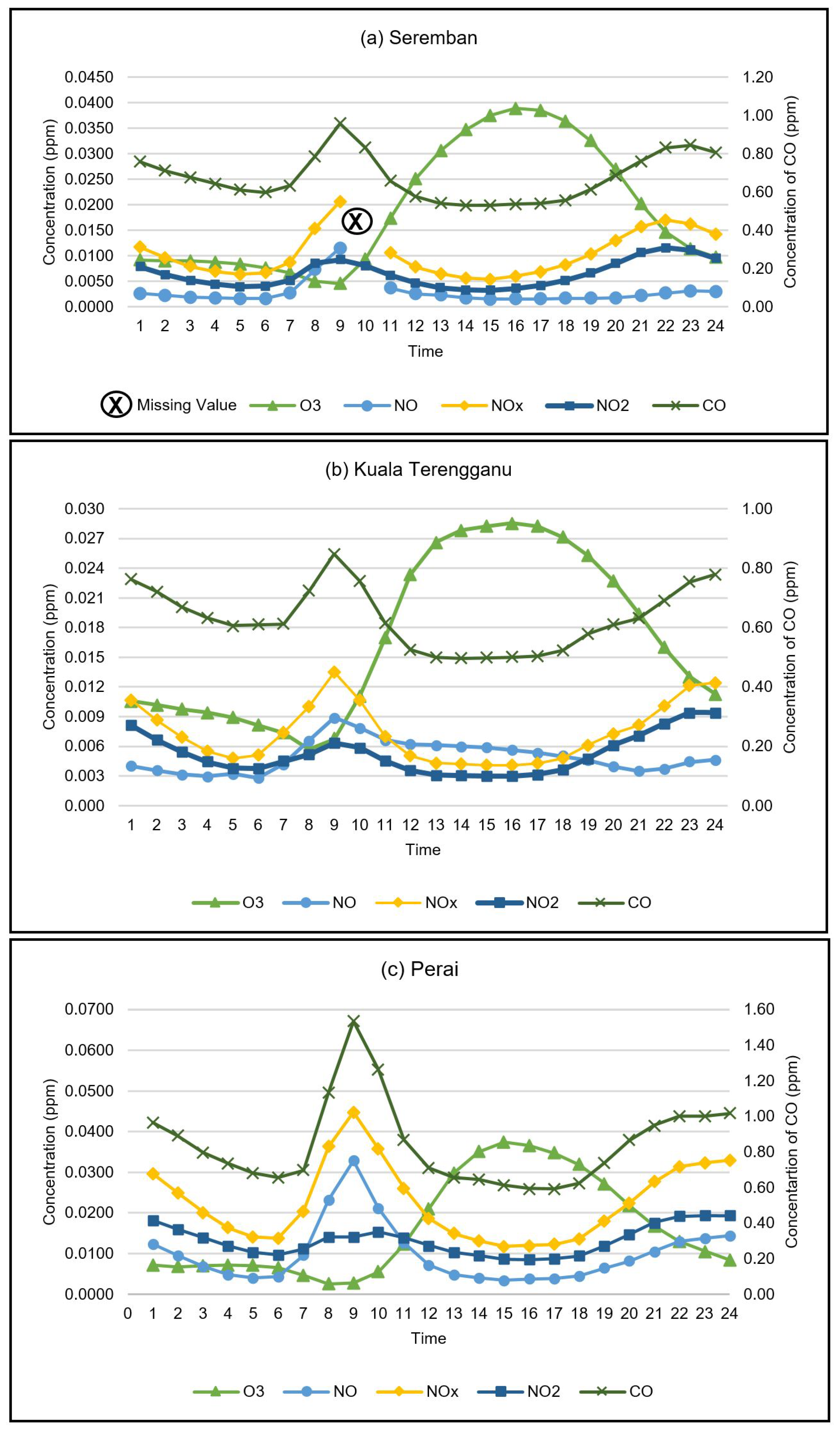
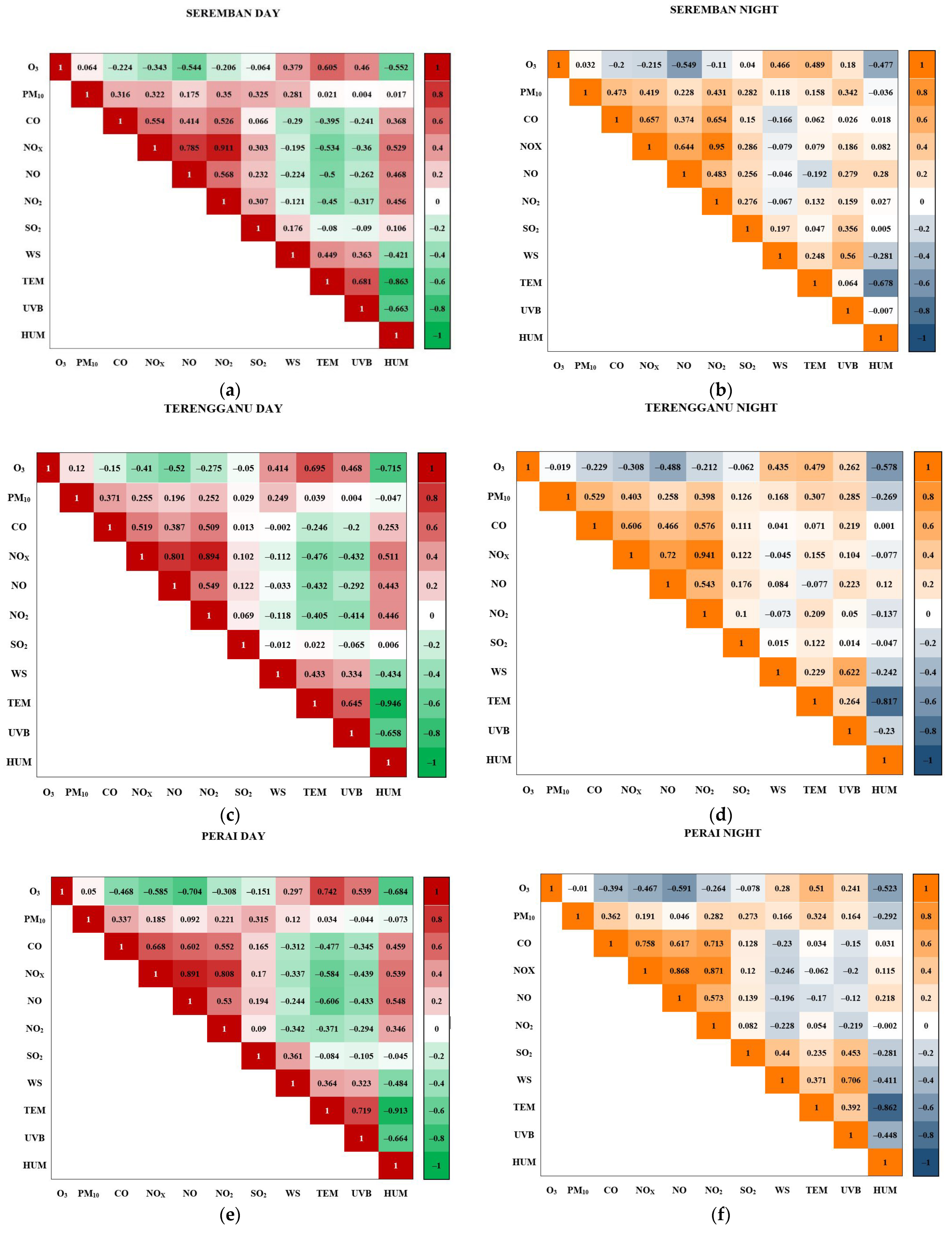
3.2. Association of O₃ Level with Its Precursors

Figure 5 shows the diurnal pattern of ground-level O₃ and its precursors, namely, NO, NO_x, NO₂, and CO, at all monitoring stations. Generally, a similar pattern of variation of O₃ levels with its precursors can be observed for all places except different intensities of pollutants. Higher concentrations of O₃ precursors, i.e., CO, NO, NO_x, and NO₂ were monitored in the morning (7:00 am to 9:00 am) and evening (6:00 pm to 10:00 pm) to coincide with people travelling to perform their daily routines. Photochemical reactions of O₃ precursors to form O₃ took place more significantly when greater solar radiation was detected during the day starting from 9:00 am. The highest O₃ formation was observed in Seremban and Seberang Perai during the maximum intensity solar radiation period (2:00 pm to 4:00 pm). O₃ concentration started to drop significantly at the night when no UVB radiation was available.

A noticeable higher concentration of NO, NO_x, and CO were observed in Perai compared with other areas. There is a lot of housing near the monitoring station and the whole Seberang Perai population was about 428,500 in 2020 [28]. The Butterworth–Kulim Express highway and North–South highway are close to the monitoring area. Furthermore, an industrial area in the Free Industrial Zone (FIZ) is also located within 5 km of the monitoring area. Hence, high air pollutant emissions from vehicles can be expected. High NO concentrations will effective atom titration of (O) in urban areas due to emissions from the large amount of transportation. The negative relationship between O₃ and NO₂ is expected as NO₂ is a precursor of O₃ [39]. This phenomenon is shown in (Equation (3)):

NO + O₃ → NO₂ + O₂

(3)

Hence, it can be seen that the O₃ levels in Perai were significantly less if compared with its precursors, i.e., NO and NO₂. If compared with Seremban and Kuala Terengganu, the least amount of NO and NO₂ were released and the amount of O₃ formation was greater compared with its precursors. The NO formed inside vehicle engines reacts with O₂ in the air to form NO₂. Ozone is formed when a combination of nitrogen (N) and O₂ is exposed to UVB by the photolysis of NO₂. ‘M’ represents an unstable molecule such as nitrogen (N₂) or O₂, and O (³P) represents an equilibrium state or low-energy oxygen atom that interacts with molecular O₂ to produce O₃ [40]:

NO₂ + hν → NO + O (³P)

(4)

O + O₂ + M → O₃ + M

(5)

Since in Seremban and Kuala Terengganu there is less NO compared with Perai, less O₃ was converted to NO₂ and O₂ as in Reaction (3). In addition, Perai has the largest value of CO due to the monitoring station being located at a main highway, and slow traffic during peak hours influenced CO concentrations. The location located near the FIZ also contributed many pollutions to that area. While during midday, the photochemical O₃ formation consumes CO which causes O₃ concentrations to increase and CO concentrations to decrease, which explains the negative association [41].

The oxidation of trace gases in the atmosphere, such as VOCs, probably contributed to O₃ formation in this location, which was largely initiated by the reaction with OH whose concentration is controlled by the concentrations of local VOCs and NO_x [42]. The phenomenon is shown below [41]:

CO + OH → H + CO₂

(6)

H + O₂ + M → HO₂ + M

(7)

HO₂ + NO → NO₂ + OH

(8)

Then, NO₂ undergoes photolysis and O₃ is formed according to Reactions (4) and (5).

3.3. Association of O₃ Level with Other Trace Gases and Weather Parameters

Figure 6 illustrates the Spearman Correlation heat matrix for daytime and nighttime in Perai, Kuala Terengganu, and Seremban. Overall, O₃ concentration was negatively correlated with its precursors, i.e., NO₂, NO_x, NO, and CO for all places during day and nighttime. While for weather parameters, the most correlated parameter was temperature followed by wind speed, UVB, and humidity. All weather parameters were positively correlated with O₃ except for humidity, which was negatively correlated. Remarkably, a moderate to strong correlation of CO with NO₂, NO_x, and NO were observed in the study areas with a higher correlation value during nighttime.

Figure 6a shows the association of daytime and nighttime O₃ levels with its precursors and weather parameters at Seremban. A moderate to strong correlation of O₃ with weather parameters during daytime was observed with the strongest positive correlation in the temperature (ρ = 0.605). A moderate negative correlation was detected with NO and a weak negative correlation of O₃ with other precursors (NO_x and CO) were calculated. A similar trend of association of O₃ levels with its precursors and weather parameters were observed during nighttime except with lower calculated ρ values. A very strong to strong correlation of NO_x with NO₂ and NO was observed during daytime and nighttime in Seremban due to its inter-convertible reaction from NO to NO₂ and reactions of NO_x with VOCs.

In Kuala Terengganu, a similar association between O₃ levels with the gases and weather parameters during daytime and nighttime was observed if compared with Seremban (Figure 6c,d). Temperature was positively correlated while humidity was negatively correlated with O₃ while its precursors also showed a negative correlation with ozone during daytime and nighttime. However, a higher calculated ρ-value between O₃ level and wind speed was calculated in Kuala Terengganu compared with other places as it is situated near the coastal area, hence land and sea breeze might have influences on air pollutant dispersion.

In Perai, the highest correlation value of CO with O₃ concentration was calculated compared with other areas with the value of −0.468. In addition, during the daytime, a strong negative correlation was observed with NO (ρ = −0.704), temperature, and humidity with ρ-values of −0.742 and −0.684, respectively, while during the nighttime, a strong negative correlation was detected with NO (ρ = −0.591). NO_x recorded a moderate correlation with O₃ that was (ρ = −0.467). CO not only had a high correlation with O₃, it also had a significant positive correlation with NO_x, NO₂, and NO compared with other areas of study with higher values observed during nighttime.

Overall, high temperature contributes to photochemical ozone chemistry which is significant in the generation of secondary aerosols such as sulfate (SO₄⁻²) and nitrate (NO₃⁻) that are generated from SO₂ and NO_x [43]. This mechanism most likely reduces the negative link between the two species over time. NO is significantly associated with O₃ concentration, as increases in its concentration are usually influenced by the complex reaction between NO_x and VOCs in the atmosphere produced by motor vehicles and industrial combustion processes [44]. Humidity is negatively correlated with O₃ due to humid days with enhanced cloud cover and thus results in a reduced photochemistry reaction in O₃ formation [42]. O₃ level has a positive association with temperature due to its formation requiring high UV radiation. Conversely, temperature is negatively correlated with humidity resulting in less humidity in the ambient air with the increase in temperature [43]. Obviously in Perai, SO₂ concentration is among the highest associated with O₃ compared with other places due to industrial areas being located near the monitoring station. According to Latif et al. [45], the fluctuations of SO₂ in the study area may be due to the contributions of SO₂ from local and regional sources of biomass burning. As Penang Port is near the monitoring areas, it might be the cause of the high concentrations of SO₂ in that area. The distribution of SO₂ is influenced by the shipping port because it transfers SO₂ to the surrounding areas [46].

In conclusion, parameters that had moderate to strong correlation (ρ ≥ 0.4) with O₃ level were used as input for daytime and nighttime prediction of O₃ levels. In the next section, the performances of the linear and nonlinear models were compared and evaluated using several performance measures.

3.4. Prediction of Daytime and Nighttime O₃ Levels

The linear relationship of O₃ levels in daytime and nighttime at all study areas are tabulated in

Table 5. Model summary for O₃ level predictions.

Study Area	Time	Predict Hour	Model
Seremban	Daytime	Next 12 h	O3, t+12 = 0.004 + 0.477 O3 − 0.027 NO + 0 T + 0 UVB + 0 H
	Nighttime	Next 12 h	O3, t+12 = 0.047 + 0.276 O3 − 0.042 NO + 0 WS − 0.001 T + 0 H
Kuala Terengganu	Daytime	Next 12 h	O3, t+12 = 0.022 + 0.453 O3 + 0.311 NOX − 0.449 NO + 0 WS + 0 T +0 UVB + 0 H
	Nighttime	Next 12 h	O3, t+12 = 0.001 + 0.487 O3 − 0.024 NO + 0 WS + 0 T + 0 H
Perai	Daytime	Next 12 h	O3, t+12 = 0.09 + 0.403 O3 − 0.002 CO + 0.197 NOX − 0.325 NO + 0 T + 0 UVB + 0 H
	Nighttime	Next 12 h	O3, t+12 = 0.44 + 0.207 O3 + 0.002 NOX − 0.091 NO − 0.001 T + 0 H

. The independent parameters for the linear model were the parameters that were strong and moderately correlated (ρ > 0.4) with O₃ level. From the table, it can be seen that O₃ level was correlated with previous O₃ concentrations, NOx and NO. However, no relation was detected with weather parameters indicating that very minimal to no correlation between weather parameters and O₃ levels was identified using MLR. NO is a significant predictor of variables during the daytime at Seremban. However, NO and temperature are significant during the nighttime. The O₃ concentration decreased 0.027 units when the one unit of NO decreased during the daytime and 0.042 and 0.001 units of NO and temperature during nighttime. In addition, Kuala Terengganu indicated an increase of one unit of NO_x will result in an increase of 0.331 units of O₃ during the daytime and a decrease of 0.024 of NO during the nighttime. Perai showed that the increase of one unit of NO_x will result in an increase of 0.197 units of O₃. The O₃ concentration decreased about 0.002 and 0.325 when the one unit of CO and NO decreased.

Validation of MLR and ANN predictive models were performed using performance indicators.

Table 6. Predictive Model Performance.

Study Area	Time	MLR			ANN
		MAE	RMSE	r	MAE	RMSE	r
Seremban	Daytime	0.015	0.019	0.576	0.010	0.012	0.699
	Nighttime	0.014	0.015	0.615	0.005	0.006	0.753
Kuala Terengganu	Daytime	0.014	0.017	0.739	0.006	0.007	0.805
	Nighttime	0.016	0.021	0.711	0.004	0.006	0.795
Perai	Daytime	0.061	0.064	0.747	0.006	0.008	0.862
	Nighttime	0.012	0.013	0.683	0.005	0.007	0.765

shows the results of the predictive model evaluation of O₃ levels using mean absolute error (MAE), root mean squared error (RMSE), and correlation (r). Generally, ANN outperformed MLR in predicting the daytime and nighttime O₃ levels in the study areas as a lower error measurement and higher correlation value were calculated. Both of the models estimated better daytime O₃ levels compared with nighttime O₃ in Kuala Terengganu and Perai with average r differences between daytime and nighttime of 6.66% and 6.97% using MLR and ANN, respectively. Meanwhile, in Seremban, ANN predicted better nighttime O₃ levels compared with daytime and the performances of ANN was observed to be the worst in Seremban (r = 0.699) compared with other areas (r value ranging from 0.765 to 0.862). Similarly, MLR predicted better nighttime O₃ concentration (r = 0.615) and MLR prediction in Seremban was observed to be the worst compared with other places with r values ranging from 0.683 to 0.747.

Ground-level ozone is produced by nonlinear photochemical reactions involving its precursors and is affected by many factors including precursor concentrations, local meteorological conditions, air transportation, deposition, etc. These factors control the production, loss, and transformation of O₃, and thus its concentrations and spatial distribution. Hence, ANN that is a nonlinear model can better represent the complex relationship of O₃ with its precursors and weather parameters. Feed forward backpropagation neural network (FFBP) is one of the most known ANNs. In several applications, including regression problems, classification problems, or time series predictions, FFBP has been successfully implemented using single autoregressive models [47]. Each input neuron represents one of the input variables (precursors or weather parameters), which are weighted before entering the hidden layer. The output of the hidden layer is based on the output of nonlinear transfer function (sigmoid function), which is applied to modify the sum of the entering weighted values. Thus, multi-variable problems can be managed by ANN as they may describe highly nonlinear connections, such as ozone production, that were overlooked by a conventional statistical technique (e.g., regression model [21]).

4. Conclusions

In this study, three urban areas located in peninsular Malaysia were selected. Hourly air pollutants and a weather parameters dataset from 2016 to 2020 were used to analyze the spatiotemporal variation of O₃ levels and its relation to the weather parameters. Seremban recorded the highest annual concentration of O₃ levels in 2017, whereas Kuala Terengganu experienced a decrement in annual O₃ levels starting from 2016. Slightly lower concentrations were observed in 2020 due to less emission of VOCs and NO_x as a result of the total lockdown in Malaysia caused by COVID-19. The diurnal plot O₃ concentration with its precursors (NO_x, NO, NO₂, and CO) showed similar trends at the three study areas. The peak of O₃ precursors was observed during rush traffic hours in the morning and evening and O₃ formation was observed to reach its peak hour during the maximum solar intensity of the day (2:00 pm to 5:00 pm) and started to decrease steeply after 6:00 pm. The concentration of ground-level ozone varies according to the population and the location of the monitoring station. VOCs react with ozone precursors during photochemical reaction and increase concentrations of ozone while decreasing concentrations of precursors. The association of ozone and its precursors including weather parameters were tested using non-parametric correlation. Spearmen correlation was used to analyze the relation of ozone with one independent variable. The result indicates that there was a strong correlation between ozone with temperature and NO, whereas a moderate correlation between NO_x and CO was observed. A similar trend of association of O₃ levels with its precursors and weather parameters was observed during nighttime except with a lower calculated ρ value. A very strong to strong correlation of NO_x with NO₂ and NO during daytime and night-time was observed in Seremban due to its inter-convertible reaction from NO to NO₂ and reactions of NO_x with VOCs. Two predictive models, i.e., a linear model (multiple linear regression) and a nonlinear model (ANN, feed forward back propagation) were attempted to model the daytime and nighttime O₃ levels at all study areas. FFBP outperformed the prediction of O₃ levels during daytime and nighttime compared with MLR due to a better agreement between the predicted and observed measurement.

In this study, an association between daytime and nighttime O₃ levels can only be made with NO_x concentration due to the missing measurement of non-methane hydrocarbon (NmHC) that represents VOC. Excluding VOC as one of the important O₃ precursors might cause the loss of important information/findings related to a place. However, this research successfully analyzed daytime and nighttime O₃ levels with its precursors at the selected areas. Variation of nighttime O₃ levels is usually neglected because O₃ cannot be formed photochemically due to the lack of sunlight at night, and NOx will continuously react with O₃, which is hypothetically the main period of O₃ depletion. Reduced O₃ depletion because of the decline in NO_x emission would lead to the accumulation of O₃ at night, which would provide higher initial concentrations for photochemical reactions during the daytime, further leading to higher O₃ concentrations and exposure hazards at daytime. Therefore, the possible long-term effects on ecosystems caused by nighttime O₃ concentrations has important research implications. Prior to this, a long-term study of nighttime O₃ variation together with its precursors is required to determine the increment/decrement trend of this pollutant. Local authorities can strategize mitigation plans accordingly, especially by controlling anthropogenic precursors such as NO_x and VOC.

References

1. Tang, H.; Takigawa, M.; Liu, G.; Zhu, J.; Kobayashi, K. A projection of ozone-induced wheat production loss in China and India for the years 2000 and 2020 with exposure-based and flux-based approaches. Glob. Chang. Biol. 2013, 19, 2739–2752. [Google Scholar] [CrossRef] [PubMed]
2. Sharma, A.; Sharma, S.K.; Mandal, T.K. Ozone sensitivity factor NOX or NMHCs. A case study over an urban site in Delhi, India. Urban Clim. 2021, 39, 100980. [Google Scholar] [CrossRef]
3. Kelly, J.; Makar, P.A.; Plummer, D.A. Projections of mid-century summer air-quality for North America: Effects of changes in climate and precursor emissions. Atmos. Chem. Phys. 2012, 12, 5367–5390. [Google Scholar] [CrossRef] [Green Version]
4. Kulkarni, P.S.; Bortoli, D.; Domingues, A.; Silva, A.M. Surface ozone variability and trend over urban and suburban sites in Portugal. Aerosol Air Qual. 2016, 16, 138–152. [Google Scholar] [CrossRef] [Green Version]
5. An, J.; Zou, J.; Wang, J.; Lin, X.; Zhu, B. Differences in ozone photochemical characteristics between the megacity Nanjing and its suburban surroundings, Yangtze River Delta, China. Environ. Sci. Pollut. Resour. 2015, 22, 19607–19617. [Google Scholar] [CrossRef]
6. Latif, M.T.; Huey, L.S.; Juneng, L. Variations of surface ozone concentration across the Klang Valley, Malaysia. Atmos. Environ. 2012, 61, 434–445. [Google Scholar] [CrossRef]
7. Awang, N.R.; Ramli, N.A.; Yahaya, A.S.; Elbayoumi, M. High night time ground level ozone concentrations in Kemaman: NO and NO2 concentrations attributions. Aerosol Air Qual. Res. 2015, 15, 1357–1366. [Google Scholar] [CrossRef]
8. Li, X.; Rappenglueck, B. A study of model nighttime ozone bias in air quality modeling. Atmos. Environ. 2018, 195, 210–228. [Google Scholar] [CrossRef]
9. Yang, J.; Ji, Z.; Kang, S.; Zhang, Q.; Chen, X.; Lee, S.Y. Spatiotemporal variations of air pollutants in western China and their relationship to meteorological factors and emission sources. Environ. Pollut. 2019, 254, 112952. [Google Scholar] [CrossRef]
10. Li, K.; Chen, L.; Ying, F.; White, S.J.; Jang, C.; Wu, X.; Gao, X.; Hong, S.; Shen, J.; Azzi, M.; et al. Meteorological and chemical impacts on ozone formation: A case study in Hangzhou, China. Atmos. Res. 2017, 196, 40–52. [Google Scholar] [CrossRef]
11. Tong, L.; Zhang, H.; Yu, J.; He, M.; Xu, N.; Zhang, J.; Qian, F.; Feng, J.; Xiao, H. Characteristics of surface ozone and nitrogen oxides at urban, suburban and rural sites in Ningbo, China. Atmos. Res. 2017, 187, 57–68. [Google Scholar] [CrossRef]
12. Romer, P.S.; Duffey, K.C.; Wooldridge, P.J.; Edgerton, E.; Baumann, K.; Feiner, P.A.; Miller, D.O.; Brune, W.H.; Koss, A.R.; de Gouw, J.A.; et al. Effects of temperature-dependent NO x emissions on continental ozone production. Atmos. Chem. Phys. 2018, 18, 2601–2614. [Google Scholar] [CrossRef] [Green Version]
13. Mujabar, S.; Chintaginjala Venkateswara, R. Empirical models for estimating the global solar radiation of Jubail Industrial City, the Kingdom of Saudi Arabia. SN Appl. Sci. 2021, 3, 95. [Google Scholar] [CrossRef]
14. Gorai, A.K.; Tuluri, F.; Tchounwou, P.B.; Ambinakudige, S. Influence of local meteorology and NO2 conditions on ground-level ozone concentrations in the eastern part of Texas, USA. Air Quality. Atmos. Health 2015, 8, 81–96. [Google Scholar] [CrossRef] [Green Version]
15. Jamaluddin, A.F.; Tangang, F.; Chung, J.X.; Juneng, L.; Sasaki, H.; Takayabu, I. Investigating the mechanisms of diurnal rainfall variability over Peninsular Malaysia using the non-hydrostatic regional climate model. Meteorol. Atmos. Phys. 2017, 130, 611–633. [Google Scholar] [CrossRef]
16. Verma, N.; Satsangi, A.; Lakhani, A.; Kumari, K.M. Prediction of Ground level Ozone concentration in Ambient Air using Multiple Regression Analysis. J. Chemstry Biol. Phys. Sci. 2015, 5, 3685–3696. [Google Scholar]
17. Hassanzadeh, S.; Hosseinibalam, F.; Omidvari, M. Statistical methods and regression analysis of stratospheric ozone and meteorological variables in Isfahan. Phys. A Stat. Mechacnic Appl. 2008, 387, 2317–2327. [Google Scholar] [CrossRef]
18. Barrero, M.A.; Grimalt, J.O.; Canto’n, L.M. Prediction of daily ozone concentration maxima in the urban atmosphere. Chemometr. Intell. Lab. Syst. 2006, 80, 67–76. [Google Scholar] [CrossRef]
19. Banja, M.; Papanastasiou, D.K.; Poupkou, A.; Melas, D. Atmospheric Pollution Research Development of a short–term ozone prediction tool in Tirana area based on meteorological variables. Atmos. Pollut. Res. 2012, 3, 32–38. [Google Scholar] [CrossRef] [Green Version]
20. Allu, S.K.; Srinivasan, S.; Maddala, R.K.; Reddy, A.; Anupoju, G.R. Seasonal ground level ozone prediction using multiple linear regression (MLR) model. Modeling Earth Syst. Environ. 2020, 6, 1981–1989. [Google Scholar] [CrossRef]
21. Al-Alawi, S.M.; Abdul-Wahab, S.A.; Bakheit, C.S. Combining principal component regression and artificial neural networks for more accurate predictions of ground-level ozone. Environ. Modeling Softw. 2008, 23, 396–403. [Google Scholar] [CrossRef]
22. Padma, K.; Samuel Selvaraj, R.; Arputharaj, S.; Milton Boaz, B. Improved Artificial Neural Network Performance on Surface Ozone Prediction Using Principal Component Analysis. Int. J. Curr. Res. Rev. 2014, 6, 1–6. [Google Scholar]
23. Pawlak, I.; Jarosławski, J. Forecasting of surface ozone concentration by using artificial neural networks in rural and urban areas in central Poland. Atmosphere 2019, 10, 52. [Google Scholar] [CrossRef] [Green Version]
24. Aljanabi, M.; Shkoukani, M.; Hijjawi, M. Ground-level Ozone Prediction Using Machine Learning Techniques: A Case Ground-level Ozone Prediction Using Machine Learning Techniques: A Case Study in Amman, Jordan. Int. J. Autom. Comput. 2020, 17, 667–677. [Google Scholar] [CrossRef]
25. Macías-Hernández, B.A.; Tello-Leal, E.; Ramirez-Alcocer, U.M.; Hernandez-Resendiz, J.D. Particulate Matter (PM2.5) Concentration Forecasting through an Artificial Neural Network in Port City Environment. Environ. Sci. Proc. 2022, 19, 31. [Google Scholar]
26. Ghahremanloo, M.; Lops, Y.; Choi, Y.; Yeganeh, B. Deep Learning Estimation of Daily Ground-Level NO2 Concentrations from Remote Sensing Data. JGR Atmos. 2021, 126, 21. [Google Scholar]
27. Wan Mahiyuddin, W.R.; Sahani, M.; Aripin, R.; Latif, M.T.; Thach, T.Q.; Wong, C.M. Short-term effects of daily air pollution on mortality. Atmos. Environ. 2013, 65, 69–79. [Google Scholar] [CrossRef]
28. Department of Statistic 2020. Available online: https://www.dosm.gov.my/v1 (accessed on 12 May 2022).
29. Astivia, O.L.O.; Zumbo, B.D. Population models and simulation methods: The case of the Spearman rank correlation. Br. J. Math. Stat. Psychol. 2017, 70, 347–367. [Google Scholar] [CrossRef]
30. Fan, Q.; Lan, J.; Liu, Y.; Wang, X.; Chan, P.; Fan, S.; Feng, Y. Diagnostic analysis of the sulfate aerosol pollution in spring over Pearl River Delta, China. Aerosol Air Qual. Res. 2015, 15, 46–57. [Google Scholar] [CrossRef] [Green Version]
31. Mukaka, M.M. Statistics corner: A guide to appropriate use of correlation coefficient in medical research. Malawi Med. J. 2012, 24, 69–71. [Google Scholar]
32. Sukatis, F.F.; Ul-Saufie, A.Z.; Noor, N.M.; Zakaria, N.A.; Suwardi, A. Estimation of Missing Values in Air Pollution Dataset by Using Various Imputation Methods. Int. J. Conserv. Sci. 2019, 10, 791–804. [Google Scholar]
33. James, G.; Witten, D.; Hastie, T.; Tibshirani, R. Springer Texts in Statistics and Introduction to Statistical Learning; Springer: Berlin, Germany, 2015. [Google Scholar] [CrossRef]
34. Ul-Saufie, A.Z.; Yahaya, A.S.; Ramli, N.A.; Hamid, H.A. Performance of multiple linear regression model for longterm PM10 concentration prediction based on gaseous and meteorological parameters. J. Appl. Sci. 2012, 12, 1488–1494. [Google Scholar] [CrossRef]
35. Kavassalis, S.C.; Murphy, J.G. Understanding ozone-meteorology correlations: A role for dry deposition. Geophys. Res. Lett. 2017, 44, 2922–2931. [Google Scholar] [CrossRef]
36. Ghosh, D.; Lal, S.; Sarkar, U. High nocturnal ozone levels at a surface site in Kolkata, India: Trade-off between meteorology and specific nocturnal chemistry. Urban Clim. 2013, 5, 82–103. [Google Scholar] [CrossRef]
37. Jenkin, M.E. Trends in ozone concentration distributions in the UK since 1990: Local, regional and global influences. Atmos. Environ. 2008, 42, 5434–5445. [Google Scholar] [CrossRef]
38. Coyle, M.; Fowler, D.; Smith, R.I.; Weston, K.; Stedman, J.R. Quantifying the spatial distribution of surface ozone concentration in the UK. Atmos. Environ. 2002, 36, 1013–1024. [Google Scholar] [CrossRef]
39. Latif, M.T.; Dominick, D.; Ahamad, F.; Shuhada, N.; Khan, M.F.; Juneng, L.; Xiang, C.J.; Nadzir, M.S.M.; Robinson, A.D.; Ismail, M.; et al. Seasonal and long-term variations of surface ozone concentrations in Malaysian Borneo. Sci. Total Environ. 2016, 573, 494–504. [Google Scholar] [CrossRef] [PubMed] [Green Version]
40. Harnung, S.E.; Johnson, M.S. Chemistry and the Environment; Cambridge University Press: Cambridge, UK, 2012. [Google Scholar]
41. Munir, S.; Chen, H.; Ropkins, K. Characterising the temporal variations of ground level ozone and its relationship with traffic-related air pollutants in the UK: A quantile regression approach. Sustain. Dev. Plan. 2012, 9, 29–41. [Google Scholar]
42. Heard, D.E.; Pilling, M.J. Measurement of OH and HO2 in the troposphere. Chem. Revolut. 2003, 103, 5163–5198. [Google Scholar] [CrossRef]
43. Ding, A.J.; Fu, C.B.; Yang, X.Q.; Sun, J.N.; Zheng, L.F.; Xie, Y.N.; Kulmala, M. Ozone and fine particle in the western Yangtze River Delta: An overview of 1-year data at the SORPES station. Atmos. Chem. Phys. 2013, 13, 5813–5830. [Google Scholar] [CrossRef] [Green Version]
44. Ahamad, F.; Latif, M.T.; Tang, R.; Juneng, L.; Diminick, D.; Juahir, H. Variation of surface ozone exceedance around Klang Valley, Malaysia. Atmos. Res. 2014, 139, 126–137. [Google Scholar] [CrossRef]
45. Latif, M.T.; Dominick, D.; Ahamad, F.; Khan, M.F.; Juneng, L.; Hamzah, F.M.; Nadzir, M.S.M. Long term assessment of air quality from a background station on the Malaysian Peninsular. Sci. Total Environ. 2014, 482, 336–348. [Google Scholar] [CrossRef]
46. Mohtar, A.A.A.; Latif, M.T.; Baharudin, N.H.; Ahamad, F.; Chung, J.X.; Othman, M.; Juneng, L. Variation of major air pollutants in different seasonal conditions in an urban environment in Malaysia. Geosci. Lett. 2018, 5, 21. [Google Scholar] [CrossRef]
47. Xu, W.Y.; Zhao, C.S.; Ran, L.; Deng, Z.Z.; Liu, P.F.; Ma, N.; Chen, L.L. Characteristics of pollutants and their correlation to meteorological conditions at a suburban site in the North China Plain. Atmos. Chem. Phys. 2011, 11, 4353–4369. [Google Scholar] [CrossRef]
Figure 1. Modeling framework.
Atmosphere 13 01780 g001
Figure 2. Hourly box plot of O3 levels in Seremban, Perai, and Kuala Terengganu. The asterisk (*) on the boxplot indicate the extreme outlier that lie >1.5 times the size of the box.
Atmosphere 13 01780 g002
Figure 3. Monthly contour plot and wind rose diagram of ground-level O3 in Seremban, Kuala Terengganu and Perai.
Atmosphere 13 01780 g003aAtmosphere 13 01780 g003b
Figure 4. Diurnal plot of O3 level during weekdays and weekends. The asterisk (*) on the boxplot indicate the extreme outlier that lie >1.5 times the size of the box.
Atmosphere 13 01780 g004
Figure 5. Diurnal plot of O3 precursors in (a) Seremban, (b) Kuala Terengganu, and (c) Perai.
Atmosphere 13 01780 g005
Figure 6. Spearman correlation matrix of O3 with trace gases and weather parameters: (a) Seremban daytime, (b) Seremban nighttime, (c) Kuala Terengganu daytime, (d) Kuala Terengganu nighttime, (e) Perai daytime, and (f) Perai nighttime.
Atmosphere 13 01780 g006