

Enhancing Rainfall-Runoff Simulation via Meteorological Variables and a Deep-Conceptual Learning-Based Framework

 , ,
, ,  ,
, 
 and
and 
Abstract
1. Introduction
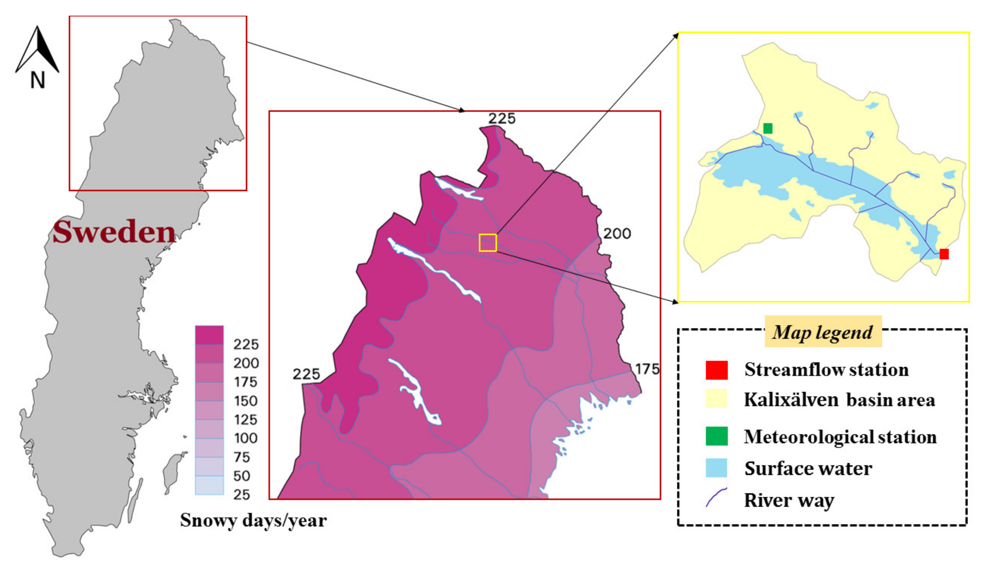
2. Study Area
3. Materials and Methods
3.1. Conceptual Phase via MISD: Modello Idrologico Semi-Distribuito in Continuo
3.2. Deep Learning Phase
3.3. Performance Assessment
4. Results
4.1. Assessment of Conceptual Streamflow Simulation
4.2. Hybrid Phase Based on the Deep Conceptual Learning Framework
5. Discussion
6. Conclusions
- Adding meteorological variables as external elements to a conceptual hydrological model is highly effective and outperforms the ordinary MISD model in streamflow simulation.
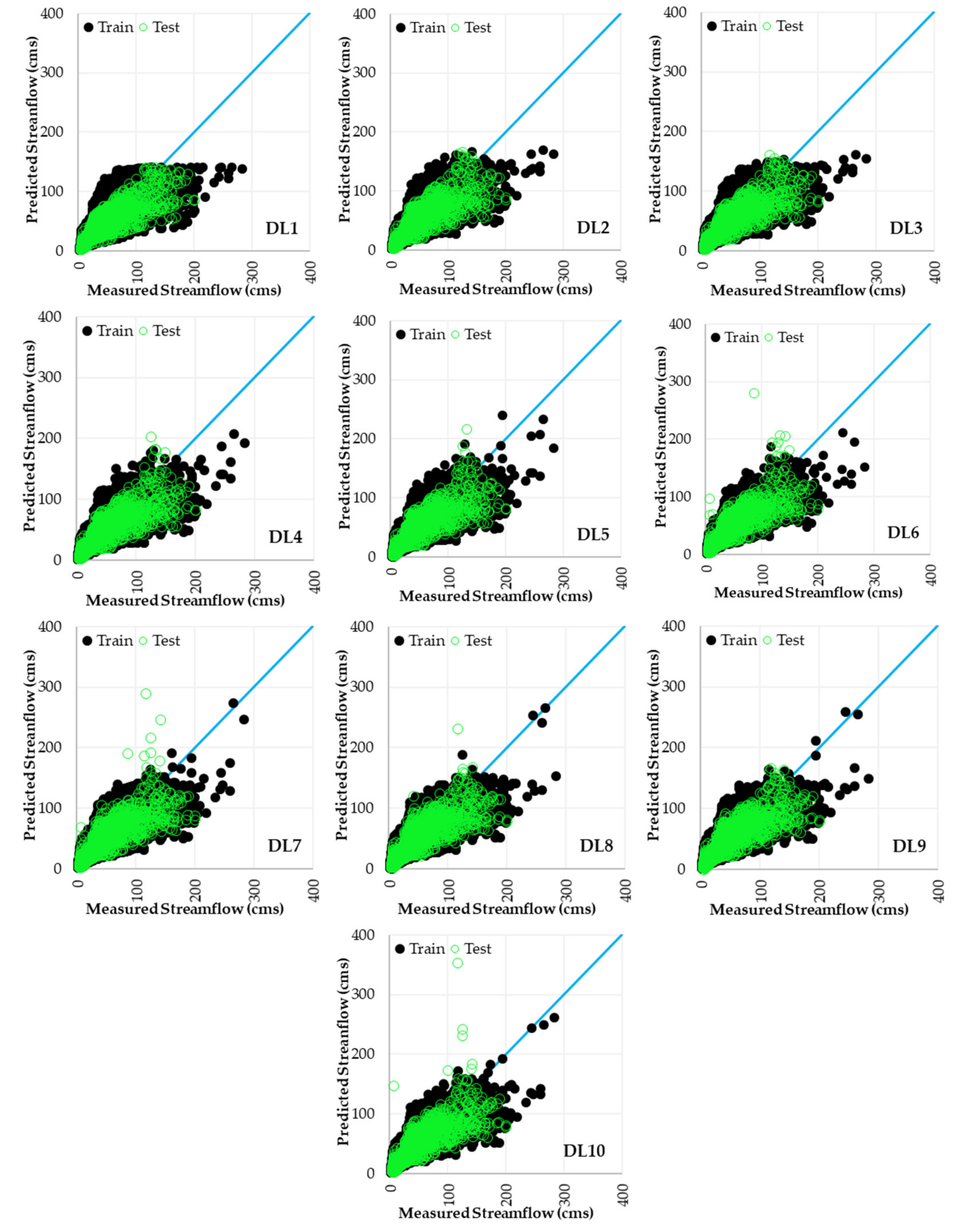
- The GMDH enhanced the accuracy of MISD for runoff simulation tasks in a snow-covered basin; the best results achieved via DL9 structures by MAE, r, and NSE throughout the testing phase were 7.89, 0.90, and 0.80 in Kalixälven hydrometric station.
- All of the employed meteorological variables improved the accuracy of streamflow simulation, and generally, adding the mean, minimum, and maximum air temperature, dew point temperature, precipitation, relative humidity, evapotranspiration, global solar radiation, and sunshine duration simulated streamflow better than the other implemented scenarios.
Author Contributions
Funding
Institutional Review Board Statement
Informed Consent Statement
Data Availability Statement
Conflicts of Interest
References
- Berhane, S.; Zemadim, B.; Haile, D.; Melesse, A. Understanding runoff generation processes and rainfall runoff modelling in the Meja watershed of Ethiopia. NBDC Tech. Rep. 2013. Available online: https://hdl.handle.net/10568/34264 (accessed on 11 October 2022).
- Breinl, K.; Lun, D.; Müller-Thomy, H.; Blöschl, G. Understanding the relationship between rainfall and flood probabilities through combined intensity-duration-frequency analysis. J. Hydrol. 2021, 602, 126759. [Google Scholar] [CrossRef]
- Zhang, K.; Wang, S.; Bao, H.; Zhao, X. Characteristics and influencing factors of rainfall-induced landslide and debris flow hazards in Shaanxi Province, China. Nat. Hazards Earth Syst. Sci. 2019, 19, 93–105. [Google Scholar] [CrossRef]
- Gao, C.; Hao, M.; Chen, J.; Gu, C. Simulation and design of joint distribution of rainfall and tide level in Wuchengxiyu Region, China. Urban Clim. 2021, 40, 101005. [Google Scholar] [CrossRef]
- Parisouj, P.; Mokari, E.; Mohebzadeh, H.; Goharnejad, H.; Jun, C. Physics-informed data-driven model for predicting streamflows: A case study of the Voshmgir Basin, Iran. Appl. Sci. 2022, 12, 7464. [Google Scholar] [CrossRef]
- Kirchner, J. Characterizing nonlinear, nonstationary, and heterogeneous hydrological response using ensemble rainfall-runoff analysis. AGU Fall Meet. Abstr. 2021, 2021, H13E-07. [Google Scholar]
- Mohammadi, B.; Moazenzadeh, R.; Christian, K.; Duan, Z. Improving streamflow simulation by combining hydrological process-driven and artificial intelligence-based models. Environ. Sci. Pollut. Res. 2021, 28, 65752–65768. [Google Scholar] [CrossRef]
- Mohammadi, B.; Safari, M.J.S.; Vazifehkhah, S. IHACRES, GR4J and MISD-based multi conceptual-machine learning approach for rainfall-runoff modeling. Sci. Rep. 2022, 12, 12096. [Google Scholar] [CrossRef]
- Qi, M.; Zhang, G.P. An investigation of model selection criteria for neural network time series forecasting. Eur. J. Oper. Res. 2001, 132, 666–680. [Google Scholar] [CrossRef]
- Hochreiter, S.; Schmidhuber, J. Long short-term memory. Neural Comput. 1997, 9, 1735–1780. [Google Scholar] [CrossRef]
- Wu, X.; Liu, Z.; Yin, L.; Zheng, W.; Song, L.; Tian, J.; Yang, B.; Liu, S. A Haze Prediction Model in Chengdu Based on LSTM. Atmosphere 2021, 12, 1479. [Google Scholar] [CrossRef]
- Adnan, R.M.; Petroselli, A.; Heddam, S.; Santos, C.A.G.; Kisi, O. Short term rainfall-runoff modelling using several machine learning methods and a conceptual event-based model. Stoch. Environ. Res. Risk Assess. 2021, 35, 597–616. [Google Scholar] [CrossRef]
- Shishegar, S.; Ghorbani, R.; Saoud, L.S.; Duchesne, S.; Pelletier, G. Rainfall–runoff modelling using octonion-valued neural networks. Hydrol. Sci. J. 2021, 66, 1857–1865. [Google Scholar] [CrossRef]
- Yokoo, K.; Ishida, K.; Nagasato, T.; Ercan, A.; Tu, T. Comparison of three recurrent neural networks for rainfall-runoff modelling at a snow-dominated watershed. IOP Conf. Ser. Earth Environ. Sci. 2021, 851, 012012. [Google Scholar] [CrossRef]
- Shao, Y.; Zhao, J.; Xu, J.; Fu, A.; Li, M. Application of rainfall-runoff simulation based on the NARX dynamic neural network model. Water 2022, 14, 2082. [Google Scholar] [CrossRef]
- Van, S.P.; Le, H.M.; Thanh, D.V.; Dang, T.D.; Loc, H.H.; Anh, D.T. Deep learning convolutional neural network in rainfall–runoff modelling. J. Hydroinformatics 2020, 22, 541–561. [Google Scholar] [CrossRef]
- Yang, T.; Sun, F.; Gentine, P.; Liu, W.; Wang, H.; Yin, J.; Du, M.; Liu, C. Evaluation and machine learning improvement of global hydrological model-based flood simulations. Environ. Res. Lett. 2019, 14, 114027. [Google Scholar] [CrossRef]
- Konapala, G.; Kao, S.-C.; Painter, S.L.; Lu, D. Machine learning assisted hybrid models can improve streamflow simulation in diverse catchments across the conterminous US. Environ. Res. Lett. 2020, 15, 104022. [Google Scholar] [CrossRef]
- Sferratore, A.; Billen, G.; Garnier, J.; Smedberg, E.; Humborg, C.; Rahm, L. Modelling nutrient fluxes from sub-arctic basins: Comparison of pristine vs. dammed rivers. J. Mar. Syst. 2008, 73, 236–249. [Google Scholar] [CrossRef]
- Brocca, L.; Melone, F.; Moramarco, T. Distributed rainfall-runoff modelling for flood frequency estimation and flood forecasting. Hydrol. Process. 2011, 25, 2801–2813. [Google Scholar] [CrossRef]
- Masseroni, D.; Cislaghi, A.; Camici, S.; Massari, C.; Brocca, L. A reliable rainfall–runoff model for flood forecasting: Review and application to a semi-urbanized watershed at high flood risk in Italy. Hydrol. Res. 2017, 48, 726–740. [Google Scholar] [CrossRef]
- Brocca, L.; Melone, F.; Moramarco, T.; Singh, V.P. A continuous rainfall-runoff model as tool for the critical hydrological scenario assessment in natural channels. In From Headwater to the Ocean. Hydrological Changes and Managements; Taniguchi, M., Bur-nett, W.C., Fukushima, Y., Haigh, M., Umezawa, Y., Eds.; Taylor & Francis Group: London, UK, 2008; pp. 175–179. [Google Scholar]
- Ivakhnenko, A.G. Heuristic self-organization in problems of engineering cybernetics. Automatica 1970, 6, 207–219. [Google Scholar] [CrossRef]
- Teng, G.; Xiao, J.; He, Y.; Zheng, T.; He, C. Use of group method of data handling for transport energy demand modeling. Energy Sci. Eng. 2017, 5, 302–317. [Google Scholar] [CrossRef]
- Nariman-Zadeh, N.; Darvizeh, A.; Darvizeh, M.; Gharababaei, H. Modelling of explosive cutting process of plates using GMDH-type neural network and singular value decomposition. J. Mater. Process. Technol. 2002, 128, 80–87. [Google Scholar] [CrossRef]
- Choi, J.; Won, J.; Jang, S.; Kim, S. Learning Enhancement Method of Long Short-Term Memory Network and Its Applicability in Hydrological Time Series Prediction. Water 2022, 14, 2910. [Google Scholar] [CrossRef]
- Li, X.; Zhang, L.; Zeng, S.; Tang, Z.; Liu, L.; Zhang, Q.; Tang, Z.; Hua, X. Predicting Monthly Runoff of the Upper Yangtze River Based on Multiple Machine Learning Models. Sustainability 2022, 14, 11149. [Google Scholar] [CrossRef]
- Mohammadi, B. A Review on the Applications of Machine Learning for Runoff Modeling. Sustain. Water Resour. Manag. 2021, 7, 98. [Google Scholar] [CrossRef]
- Singh, A.K.; Kumar, P.; Ali, R.; Al-Ansari, N.; Vishwakarma, D.K.; Kushwaha, K.S.; Panda, K.C.; Sagar, A.; Mirzania, E.; Elbeltagi, A.; et al. An Integrated Statistical-Machine Learning Approach for Runoff Prediction. Sustainability 2022, 14, 8209. [Google Scholar] [CrossRef]
- Guan, Y.; Mohammadi, B.; Pham, Q.B.; Adarsh, S.; Balkhair, K.S.; Rahman, K.U.; Linh, N.T.T.; Tri, D.Q. A Novel Approach for Predicting Daily Pan Evaporation in the Coastal Regions of Iran Using Support Vector Regression Coupled with Krill Herd Algorithm Model. Theor. Appl. Climatol. 2020, 142, 349–367. [Google Scholar] [CrossRef]
- Li, P.; Zhang, J.; Krebs, P. Prediction of Flow Based on a CNN-LSTM Combined Deep Learning Approach. Water 2022, 14, 993. [Google Scholar] [CrossRef]
- Contreras, P.; Orellana-Alvear, J.; Muñoz, P.; Bendix, J.; Célleri, R. Influence of Random Forest Hyperparameterization on Short-Term Runoff Forecasting in an Andean Mountain Catchment. Atmosphere 2021, 12, 238. [Google Scholar] [CrossRef]
- Jung, K.; Kim, E.; Kang, B. Estimation of Low-Flow in South Korean River Basins Using a Canonical Correlation Analysis and Neural Network (CCA-NN) Based Regional Frequency Analysis. Atmosphere 2019, 10, 695. [Google Scholar] [CrossRef]
- Mehdizadeh, S.; Mohammadi, B.; Ahmadi, F. Establishing Coupled Models for Estimating Daily Dew Point Temperature Using Nature-Inspired Optimization Algorithms. Hydrology 2022, 9, 9. [Google Scholar] [CrossRef]
- Seo, Y.; Kim, S.; Singh, V. Machine Learning Models Coupled with Variational Mode Decomposition: A New Approach for Modeling Daily Rainfall-Runoff. Atmosphere 2018, 21qas, 251. [Google Scholar] [CrossRef]
- Ávila, L.; Silveira, R.; Campos, A.; Rogiski, N.; Gonçalves, J.; Scortegagna, A.; Freita, C.; Aver, C.; Fan, F. Comparative Evaluation of Five Hydrological Models in a Large-Scale and Tropical River Basin. Water 2022, 14, 3013. [Google Scholar] [CrossRef]
- Okiria, E.; Okazawa, H.; Noda, K.; Kobayashi, Y.; Suzuki, S.; Yamazaki, Y. A Comparative Evaluation of Lumped and Semi-Distributed Conceptual Hydrological Models: Does Model Complexity Enhance Hydrograph Prediction? Hydrology 2022, 9, 89. [Google Scholar] [CrossRef]
- Flores, N.; Rodríguez, R.; Yépez, S.; Osores, V.; Rau, P.; Rivera, D.; Balocchi, F. Comparison of Three Daily Rainfall-Runoff Hydrological Models Using Four Evapotranspiration Models in Four Small Forested Watersheds with Different Land Cover in South-Central Chile. Water 2021, 13, 3191. [Google Scholar] [CrossRef]
- Moustakas, S.; Willems, P. Testing the Efficiency of Parameter Disaggregation for Distributed Rainfall-Runoff Modelling. Water 2021, 13, 972. [Google Scholar] [CrossRef]
- Rahman, K.U.; Pham, Q.B.; Jadoon, K.Z.; Shahid, M.; Kushwaha, D.P.; Duan, Z.; Mohammadi, B.; Khedher, K.M.; Anh, D.T. Comparison of Machine Learning and Process-Based SWAT Model in Simulating Streamflow in the Upper Indus Basin. Appl. Water Sci. 2022, 12, 178. [Google Scholar] [CrossRef]
- Fang, Y.; Huang, Y.; Qu, B.; Zhang, X.; Zhang, T.; Xia, D. Estimating the Routing Parameter of the Xin’anjiang Hydrological Model Based on Remote Sensing Data and Machine Learning. Remote Sens. 2022, 14, 4609. [Google Scholar] [CrossRef]
- Li, S.; Liu, C.H.; Lin, Q.; Wen, Q.; Su, L.; Huang, G.; Ding, Z. Deep Residual Correction Network for Partial Domain Adaptation. IEEE Trans. Pattern Anal. Mach. Intell. 2020, 43, 2329–2344. [Google Scholar] [CrossRef] [PubMed]
- Yin, L.; Wang, L.; Keim, B.D.; Konsoer, K.; Zheng, W. Wavelet Analysis of Dam Injection and Discharge in Three Gorges Dam and Reservoir with Precipitation and River Discharge. Water 2022, 14, 567. [Google Scholar] [CrossRef]
- Ditthakit, P.; Pinthong, S.; Salaeh, N.; Binnui, F.; Khwanchum, L.; Pham, Q.B. Using Machine Learning Methods for Supporting GR2M Model in Runoff Estimation in an Ungauged Basin. Sci. Rep. 2021, 11, 19955. [Google Scholar] [CrossRef] [PubMed]
- Ebtehaj, I.; Sammen, S.S.; Sidek, L.M.; Malik, A.; Sihag, P.; Al-Janabi, A.M.S.; Chau, K.-W.; Bonakdari, H. Prediction of Daily Water Level Using New Hybridized GS-GMDH and ANFIS-FCM Models. Eng. Appl. Comput. Fluid Mech. 2021, 15, 1343–1361. [Google Scholar] [CrossRef]
- Aghelpour, P.; Bahrami-Pichaghchi, H.; Karimpour, F. Estimating Daily Rice Crop Evapotranspiration in Limited Climatic Data and Utilizing the Soft Computing Algorithms MLP, RBF, GRNN, and GMDH. Complexity 2022, 2022, 4534822. [Google Scholar] [CrossRef]
- Khodakhah, H.; Aghelpour, P.; Hamedi, Z. Comparing Linear and Non-Linear Data-Driven Approaches in Monthly River Flow Prediction, Based on the Models SARIMA, LSSVM, ANFIS, and GMDH. Environ. Sci. Pollut. Res. 2021, 29, 21935–21954. [Google Scholar] [CrossRef]
- Hadadi, F.; Moazenzadeh, R.; Mohammadi, B. Estimation of Actual Evapotranspiration: A Novel Hybrid Method Based on Remote Sensing and Artificial Intelligence. J. Hydrol. 2022, 609, 127774. [Google Scholar] [CrossRef]
- Ebtehaj, I.; Bonakdari, H.; Gharabaghi, B. A Reliable Linear Method for Modeling Lake Level Fluctuations. J. Hydrol. 2019, 570, 236–250. [Google Scholar] [CrossRef]
- Li, J.; Qian, K.; Liu, Y.; Yan, W.; Yang, X.; Luo, G.; Ma, X. LSTM-Based Model for Predicting Inland River Runoff in Arid Region: A Case Study on Yarkant River, Northwest China. Water 2022, 14, 1745. [Google Scholar] [CrossRef]
- Ren, Y.; Zeng, S.; Liu, J.; Tang, Z.; Hua, X.; Li, Z.; Song, J.; Xia, J. Mid- to Long-Term Runoff Prediction Based on Deep Learning at Different Time Scales in the Upper Yangtze River Basin. Water 2022, 14, 1692. [Google Scholar] [CrossRef]
- Filho, F.J.M.N.; de Assis Souza Filho, F.; Porto, V.C.; Rocha, R.V.; Estácio, Á.B.S.; Martins, E.S.P.R. Deep Learning for Streamflow Regionalization for Ungauged Basins: Application of Long-Short-Term-Memory Cells in Semiarid Regions. Water 2022, 14, 1318. [Google Scholar] [CrossRef]
- Chen, X.; Huang, J.; Wang, S.; Zhou, G.; Gao, H.; Liu, M.; Yuan, Y.; Zheng, L.; Li, Q.; Qi, H. A New Rainfall-Runoff Model Using Improved LSTM with Attentive Long and Short Lag-Time. Water 2022, 14, 697. [Google Scholar] [CrossRef]
- Wakatsuki, Y.; Nakane, H.; Hashino, T. River Stage Modeling with a Deep Neural Network Using Long-Term Rainfall Time Series as Input Data: Application to the Shimanto-River Watershed. Water 2022, 14, 452. [Google Scholar] [CrossRef]
- Roy, B.; Singh, M.P.; Kaloop, M.R.; Kumar, D.; Hu, J.-W.; Kumar, R.; Hwang, W.-S. Data-Driven Approach for Rainfall-Runoff Modelling Using Equilibrium Optimizer Coupled Extreme Learning Machine and Deep Neural Network. Appl. Sci. 2021, 11, 6238. [Google Scholar] [CrossRef]
- Li, Z.; Kang, L.; Zhou, L.; Zhu, M. Deep Learning Framework with Time Series Analysis Methods for Runoff Prediction. Water 2021, 13, 575. [Google Scholar] [CrossRef]
- Liu, Y.; Zhang, T.; Kang, A.; Li, J.; Lei, X. Research on Runoff Simulations Using Deep-Learning Methods. Sustainability 2021, 13, 1336. [Google Scholar] [CrossRef]
- Hu, C.; Wu, Q.; Li, H.; Jian, S.; Li, N.; Lou, Z. Deep Learning with a Long Short-Term Memory Networks Approach for Rainfall-Runoff Simulation. Water 2018, 10, 1543. [Google Scholar] [CrossRef]
- Fan, H.; Jiang, M.; Xu, L.; Zhu, H.; Cheng, J.; Jiang, J. Comparison of Long Short Term Memory Networks and the Hydrological Model in Runoff Simulation. Water 2020, 12, 175. [Google Scholar] [CrossRef]
- Huang, C.-L.; Hsu, N.-S.; Wei, C.-C. Coupled Heuristic Prediction of Long Lead-Time Accumulated Total Inflow of a Reservoir during Typhoons Using Deterministic Recurrent and Fuzzy Inference-Based Neural Network. Water 2015, 7, 6516–6550. [Google Scholar] [CrossRef]
- de la Fuente, A.; Meruane, V.; Meruane, C. Hydrological Early Warning System Based on a Deep Learning Runoff Model Coupled with a Meteorological Forecast. Water 2019, 11, 1808. [Google Scholar] [CrossRef]
- Iqbal, Z.; Shahid, S.; Ismail, T.; Sa’adi, Z.; Farooque, A.; Yaseen, Z.M. Distributed Hydrological Model Based on Machine Learning Algorithm: Assessment of Climate Change Impact on Floods. Sustainability 2022, 14, 6620. [Google Scholar] [CrossRef]


| Variable | Abbreviation | Unit | Mean | Minimum | Maximum | Standard Error | Median | Standard Deviation | Kurtosis | Skewness |
|---|---|---|---|---|---|---|---|---|---|---|
| Temperature | T | °C | −0.48 | −37.80 | 24.40 | 0.08 | −0.10 | 10.23 | −0.37 | −0.33 |
| Minimum temperature | Tmin | °C | −4.84 | −40.10 | 18.40 | 0.09 | −3.30 | 10.70 | −0.46 | −0.48 |
| Maximum temperature | Tmax | °C | 3.59 | −35.20 | 30.30 | 0.08 | 3.20 | 10.36 | −0.40 | −0.12 |
| Dew point temperature | Tdew | °C | −4.315 | −42.24 | 17.08 | 0.07 | −3.67 | 9.27 | −0.11 | −0.44 |
| Relative humidity | RH | % | 75.23 | 30 | 100 | 0.09 | 75.83 | 11.62 | −0.45 | −0.26 |
| Global solar radiation | GSR | W/m2 | 90.86 | 0.00 | 363.87 | 0.78 | 61.22 | 91.01 | −0.35 | 0.84 |
| Sunshine duration | SSD | h | 3.98 | 0.00 | 24 | 0.04 | 1.66 | 4.96 | 0.86 | 1.26 |
| Atmospheric pressure | AP | Pascal | 1009.13 | 948.49 | 1051.71 | 0.10 | 1009.79 | 12.08 | 0.51 | −0.28 |
| Precipitation | P | mm | 1.44 | 0.00 | 40 | 0.03 | 0.00 | 3.59 | 25.91 | 4.46 |
| Evapotranspiration | ET | mm | 1.29 | 0.00 | 6.08 | 0.005 | 1.31 | 0.61 | 1.24 | 0.10 |
| Streamflow | Q | cms | 30.20 | 2.43 | 284 | 0.29 | 15.3 | 34.59 | 4.66 | 20 |
| Parameters | Description | Optimal Value |
|---|---|---|
| W_max | Fixed water capacity of 1st layer | 150 |
| W_max2 | Total water capacity of 2nd layer | 731.503 |
| W_p | Initial conditions (fraction of W_max) | 0.797 |
| m2 | The exponent of drainage for 1st layer | 4.827 |
| Ks | Hydraulic conductivity for 1st layer | 8.528 |
| gamma1 | Coefficient lag-time relationship | 3.5 |
| Kc | Parameter of potential evapotranspiration | 0.4 |
| alpha | Exponent runoff | 6.022 |
| Cm | Snow module parameter degree-day | 0.878 |
| m22 | The exponent of drainage for 2nd layer | 5 |
| Ks2 | Hydraulic conductivity for 2nd layer | 65 |
| Stage | MAE | NSE | r |
|---|---|---|---|
| Calibration | 9.7 | 0.69 | 0.85 |
| Validation | 8.33 | 0.77 | 0.88 |
| No. | Phase | Inputs | Output | Model |
|---|---|---|---|---|
| 1 | Coupled DL phase by MISD | Q (MISD), P | Q | DL1 |
| 2 | Q (MISD), P, T | Q | DL2 | |
| 3 | Q (MISD), P, T, Tmax | Q | DL3 | |
| 4 | Q (MISD), P, T, Tmax, Tmin | Q | DL4 | |
| 5 | Q (MISD), P, T, Tmax, Tmin, Tdew | Q | DL5 | |
| 6 | Q (MISD), P, T, Tmax, Tmin, Tdew, ET | Q | DL6 | |
| 7 | Q (MISD), P, T, Tmax, Tmin, Tdew, ET, GSR | Q | DL7 | |
| 8 | Q (MISD), P, T, Tmax, Tmin, Tdew, ET, GSR, SSH | Q | DL8 | |
| 9 | Q (MISD), P, T, Tmax, Tmin, Tdew, ET, GSR, SSH, RH | Q | DL9 | |
| 10 | Q (MISD), P, T, Tmax, Tmin, Tdew, ET, GSR, SSH, RH, AP | Q | DL10 |
| Phase | Training | Testing | ||||
|---|---|---|---|---|---|---|
| Model | MAE | NSE | r | MAE | NSE | r |
| DL1 | 9.19 | 0.75 | 0.87 | 8.26 | 0.79 | 0.89 |
| DL2 | 8.73 | 0.77 | 0.88 | 8.11 | 0.80 | 0.89 |
| DL3 | 8.72 | 0.77 | 0.88 | 8.11 | 0.80 | 0.90 |
| DL4 | 8.61 | 0.78 | 0.88 | 8.07 | 0.79 | 0.89 |
| DL5 | 8.54 | 0.78 | 0.88 | 8.07 | 0.79 | 0.89 |
| DL6 | 8.52 | 0.78 | 0.88 | 8.10 | 0.78 | 0.89 |
| DL7 | 8.48 | 0.79 | 0.89 | 8.20 | 0.78 | 0.89 |
| DL8 | 8.42 | 0.78 | 0.89 | 8.01 | 0.79 | 0.89 |
| DL9 | 8.44 | 0.78 | 0.89 | 7.89 | 0.80 | 0.90 |
| DL10 | 8.52 | 0.79 | 0.89 | 8.23 | 0.78 | 0.88 |
Publisher’s Note: MDPI stays neutral with regard to jurisdictional claims in published maps and institutional affiliations. |
© 2022 by the authors. Licensee MDPI, Basel, Switzerland. This article is an open access article distributed under the terms and conditions of the Creative Commons Attribution (CC BY) license (https://creativecommons.org/licenses/by/4.0/).
Share and Cite
Achite, M.; Mohammadi, B.; Jehanzaib, M.; Elshaboury, N.; Pham, Q.B.; Duan, Z. Enhancing Rainfall-Runoff Simulation via Meteorological Variables and a Deep-Conceptual Learning-Based Framework. Atmosphere 2022, 13, 1688. https://doi.org/10.3390/atmos13101688
Achite M, Mohammadi B, Jehanzaib M, Elshaboury N, Pham QB, Duan Z. Enhancing Rainfall-Runoff Simulation via Meteorological Variables and a Deep-Conceptual Learning-Based Framework. Atmosphere. 2022; 13(10):1688. https://doi.org/10.3390/atmos13101688
Chicago/Turabian StyleAchite, Mohammed, Babak Mohammadi, Muhammad Jehanzaib, Nehal Elshaboury, Quoc Bao Pham, and Zheng Duan. 2022. "Enhancing Rainfall-Runoff Simulation via Meteorological Variables and a Deep-Conceptual Learning-Based Framework" Atmosphere 13, no. 10: 1688. https://doi.org/10.3390/atmos13101688
APA StyleAchite, M., Mohammadi, B., Jehanzaib, M., Elshaboury, N., Pham, Q. B., & Duan, Z. (2022). Enhancing Rainfall-Runoff Simulation via Meteorological Variables and a Deep-Conceptual Learning-Based Framework. Atmosphere, 13(10), 1688. https://doi.org/10.3390/atmos13101688