Article

Negative Storm Surges in the Elbe Estuary—Large-Scale Meteorological Conditions and Future Climate Change

1
Federal Maritime and Hydrographic Agency (BSH), 20359 Hamburg, Germany
2
Federal Waterways Engineering and Research Institute (BAW), 22559 Hamburg, Germany
*
Author to whom correspondence should be addressed.
Atmosphere 2022, 13(10), 1634; https://doi.org/10.3390/atmos13101634
Submission received: 13 June 2022 / Revised: 16 September 2022 / Accepted: 21 September 2022 / Published: 7 October 2022

Abstract

:
Negative storm surges in the Elbe estuary can affect shipping as well as shoreline infrastructure. The significant reduction of water level caused by strong offshore winds can lead to extreme low water events, which endanger waterfront structures. The current study analyses the large-scale meteorological conditions inducing such situations and possible future changes due to climate change. The analysis is based on tide gauge data from Cuxhaven, atmospheric reanalysis data and an objective weather classification approach. It is found that south-easterly wind directions in combination with strong gales favour extreme low water events at Cuxhaven. Furthermore, the analysis of a single model large ensemble of climate projections shows a significant decrease in the frequency of such conditions for the far future (2071–2100). Regarding future global mean sea level rise the simulation results of a sensitivity study indicate that water levels during such extreme events approximately follow the development of the mean sea level rise. Therefore, our study suggests that both meteorological conditions and mean sea levels in a warmer future climate will be less favourable for the occurrence of extreme low water events in the Elbe estuary.

1. Introduction

Strong offshore winds can lead to a significant reduction in the water level in the tidally dominated German Bight and adjacent estuaries. Events like these may severely restrict transportation along the waterways and could therefore lead to economic loss. Extremely lowered water levels can also endanger the stability of waterfront structures along the shoreline due to pressure imbalance [1]. The port of Hamburg is a very important transit point and the third biggest port in Europe (after Rotterdam and Antwerp) where 128.7 million tons of seaborne cargoes were loaded or discharged in 2021 [2]. It is situated approx. 107 km inland in the Elbe estuary, which is significantly affected by tides with an average tidal range of 3.82 m measured at St. Pauli (close to the harbour) [3].
Besides this tidal variability, the occurrence of strong surface-near winds—depending on wind direction—significantly alters water levels in the Elbe estuary. Generally speaking, if wind direction roughly matches (opposes) the stream direction of the Elbe river out of the estuary, water levels are reduced (increased) relative to what would be expected from the tidal influence only. The phenomenon of wind-induced reduction of water levels during tidal low water can be referred to as storm ebb (German: “Sturmebbe”), sea level blowout [4], or negative storm surge [5]. For this study, we will use the term extreme low water (hereafter “ELW”) to address tidal low water levels (LWs) that are additionally influenced by offshore winds and hence significantly below mean low water (mLW). This is to distinguish from the solely wind-driven part of the water level reduction apart from tidal level, and which we call “negative storm surge” (NSS) in this manuscript.
Besides the term also the definition of what is considered an NSS or an ELW varies in the literature. In a number of studies, a threshold-based approach is used where every water level reduction below a certain threshold is considered an NSS (e.g., [6,7,8]). Most of these studies either consider an official threshold given by respective authorities or apply a threshold mirroring the commonly used threshold for positive storm surges at the respective gauge. Another approach is to analyse the distribution of the excess, i.e., the detrendet non-tidal residuals of the water levels ([9,10]). Other studies created an index (SSI) describing the mean of the three lowest independent NSS minima per-year, along the considered periods, e.g., [11].
The most important parameters that affect an ELW are local winds, remote winds (large-scale atmospheric circulation), astronomic tides, bathymetry of the area, currents, and waves [12]. The individual impact of these variables varies for different locations. Gurumurthy et al. [4] for example showed that the local winds affect the NSS potential further up an estuary whereas at more open locations, such as the NY Harbour [4] or the Port of Buenos Aires [7], remote winds play a more important role. In more enclosed basins, such as the Mediterranean [11] or Baltic Sea [9], an NSS is often triggered by a preceding positive storm surge (due to the effects of seiches) and generally lasts shorter than its positive counterpart. This is because the (sub-)basins fill up during the positive storm tide and induce a rapid drop in water level once the onshore wind forcing vanishes.
Local topographic conditions can also have an influence on the occurrence of NSSs. It might determine whether the surge is triggered by fast-moving strong storms, as it is the case for the port of Buenos Aires [7], the Baltic [9] and the North-East US coast [13], or rather by long-lasting and stationary atmospheric pressure systems which would be the case in Alaska [8] or the southern North Sea coast of the Netherlands [9].
To our knowledge, possible future changes in NSSs have been very rarely analysed in scientific literature. Conte et al. [11] found that the effect of climate change in this respect is small for the Mediterranean Sea.
In the presence of ongoing global warming, the related global sea-level rise (SLR) is of particular relevance for phenomena such as NSSs and resulting ELWs. The most comprehensive overview on projections of future global mean SLR is given in the IPCC 6th Assessment Report (AR6) [14]. For the majority of coastal regions, the median of future regional mean SLR lies within ±20 cm of the median of the projected global mean SLR until 2100 [13]. Projections for individual tide gauge locations can be accessed via an interactive tool hosted by NASA [14,15,16]. At the gauge Cuxhaven (located in the mouth of the Elbe estuary), the projected SLR for year 2050 relative to the reference period 1995-2014 is in the range between 0.25 and 0.29 m for the median of all SSP-scenarios [14,15,16]. However, for the year 2100 the projected SLR is strongly differing across socio-economic pathways (SSPs) and associated emission scenarios, with a median and 66% confidence interval of (i) 0.51(0.32-- 0.74) m for SSP1-2.6, (ii) 0.64 (0.46–0.88) m for SSP2-4.5, (iii) 0.73 (0.52–1.00) m for SSP3-7.0, and (iv) 0.85 (0.61–1.16) m for SSP5-8.5 [14,15,16]. The median of the projections of regional mean SLR at Cuxhaven is up to 8 cm higher than the median of global mean SLR [14,15,16].
As future SLR will influence water level and therefore ELW in the Elbe estuary, the range and development of projected SLR needs to be considered in our investigation. To assess SLR impacts in estuaries, advanced hydrodynamic numerical models are used as a common tool which can consider various driving forces and their interaction. In a review of [17] several hydrodynamic numerical studies on the effect of SLR on estuarine parameters and processes are summarised. For the Elbe estuary, the impact of SLR on storm tides [18] and mean tidal parameters [19] was investigated. However, to our knowledge, the impact of SLR on ELWs in the Elbe estuary has not yet been studied.
Future changes in atmospheric circulation have already been analysed in a number of studies: In the recent past, a shift to more zonal rather than meridional flow over most parts of Northern and Central Europe has been observed [20]. This has been found to be continuing throughout different future scenarios [21]. Following this shift, there is an increase in westerly flows which can be seen in the global climate model (GCM) [22,23] as well as in higher resolution regional climate model (RCM) simulations [23,24]. This increase in westerlies goes along with a decrease in easterly flows, especially in winter [21,25,26]. Future changes in storminess on the other hand are still subject to great uncertainties.
There is a considerable number of studies focusing on positive storm surges in the North Sea area [27,28]. NSSs on the other hand are more common at the German Baltic Sea coast (e.g., [5]). To our knowledge, there are no preceding investigations on NSSs in the Elbe estuary, despite its high relevance for transport due to the connection to the Port of Hamburg.
This study aims at addressing this gap by analysing the large-scale meteorological conditions inducing past NSSs in the Elbe estuary and assessing how far the frequency of these meteorological conditions may change in a potential future climate. The water levels along the Elbe estuary are strongly influenced on the one hand by SLR and river runoff into that region and on the other hand by the large-scale atmospheric circulation and the associated wind field. It is obvious that under continued global warming, SLR will become a non-negligible factor in the context of NSS and resulting ELWs. We address this issue by additionally including a sensitivity study based on a hydrodynamic-numerical simulation to investigate the influence of possible SLR scenarios on ELW caused by a particular NSS event.
The following data and methods used in this paper are described in Section 2. Section 3 presents an analysis of past extreme low waters as well as a statistical analysis of the mean meteorological conditions before ELWs, and shows first results for possible future developments derived from an ensemble of global climate model simulations. It also contains the results of the hydrodynamic sensitivity study. These results are followed by a discussion (Section 4) and conclusions (Section 5).

2. Data and Methods

2.1. Data

2.1.1. Observational Data from Gauge Stations

As a fundamental data set for this investigation, we use observations of the low water (LW) at the gauges Cuxhaven and St. Pauli for the period 1950–2019 which are provided and checked for plausibility by the German Federal Waterways and Shipping Administration (WSV) [29]. Based on the data at Cuxhaven, we develop a definition of ELW (see Section 2.2.1). The points in time of LW levels matching our definition of an ELW form the basis for the meteorological analyses. This data set is also used to analyse and visualize the long-term development of the median and minimum LW of each year at the two gauges Cuxhaven and St Pauli.

2.1.2. Atmospheric Reanalysis Data

For the analysis of past meteorological conditions related to the identified ELWs, we use the ERA5 reanalysis which is the most recent reanalysis dataset produced by the European Centre for Medium-Range Weather Forecasts [30,31]. As such, it is one of the most modern and advanced global reanalyses, using the global weather forecasting system IFS. The ERA5 data are available on a high-resolution grid with a spacing of 0.25° and in hourly resolution for the period from 1979 to the present and are updated at regular intervals. To additionally cover the period before 1978 we included the ERA5 backward extension [32]. The only variable considered here is the sea level pressure (SLP) which is an instantaneous output, processed as follows for this investigation: (1) for daily mean values, an average is calculated of the hourly values from 0UTC to 23UTC; (2) for a better representation of the weather conditions leading up to the event, a 24-h mean is calculated as an average over the 24 h directly before the event, including the hour of the event itself.
In a comparison of several reanalyses with observational SLP data over the North Sea area [33] it was shown that the ERA reanalyses (ERA40, ERA-Interim) performed best, except for mixed sea/land grid points. Since to our knowledge there are no consistent observational data sets for both land and sea, we assume that the ERA reanalyses give the best representation in our research area, especially since the higher spatial resolution compared to NCEP and 20CR is likely to minimise the interference of mixed sea/land grid points. Further, ERA5 shows similar results regarding the occurrence of atmospheric circulation types as ERA40 and ERA-Interim (not shown). Differences (statistically insignificant) between both, the NCEP and ERA groups, can be seen for A and NW circulation, but are negligible for our investigations since negative storm surges occur almost exclusively during easterly situations. Therefore, the use of ERA5 for our investigations seems highly appropriate.

2.1.3. Climate Model Simulations

In order to analyse the potential future change of meteorological conditions favourable for ELWs in the Elbe estuary, we make use of the large ensemble produced by the Swedish Meteorological and Hydrological Institute (SMHI-LENS; [34]), employing the atmosphere-ocean general circulation model EC-Earth3 ([35]). EC-Earth3 includes a model component for the global atmosphere that is based on ECMWF’s IFS (cy36r4) as well as NEMO3.6 and LIM3 for the ocean and sea-ice, respectively. EC-Earth3 features a spectral resolution of TL255 (approx. 80 km grid spacing) and 91 levels in the vertical for the atmosphere and the tripolar ORCA1-grid with a nominal resolution of 1°—with mesh refinement along the Equator—and 75 levels for the ocean and sea-ice components.
SMHI-LENS comprises 50 simulations for each, the historical period 1970–2014 and different scenarios covering the period 2015–2100. Details about the initialisation and ensemble generation can be found in [34]. All simulations of a given experiment are subject to identical external forcings—such as greenhouse gases and aerosols—following the protocol for the historical-experiment of the Coupled Model Intercomparison Project in its sixth phase (CMIP6) [36] and ScenarioMIP [37], respectively. For the analyses presented in this study, we examined the four Tier1-scenarios of ScenarioMIP that is SSP1-2.6, SSP2-4.5, SSP3-7.0, and SSP5-8.5. These span a wide range of socio-economic narratives and greenhouse gas concentration pathways for the remainder of the 21st century. The large number of simulations available for SMHI-LENS make it an excellent tool to derive robust estimates of climate change signals projected by this model. While every single simulation is subject to natural variability superimposed on potential climate change signals, the joint analysis of the whole ensemble enables us to “average out” the internal fluctuations of the individual runs.
Our analyses were based on daily mean sea-level pressure fields taken from these simulations.

2.2. Methods

2.2.1. Definition Negative Storm Tide

In contrast to wind-induced extreme high water levels, i.e., (positive) storm tides, there is no consistent definition for wind-induced extreme low water levels. We decided to define a threshold in this respect that yields a similar frequency of events as for the (positive) storm tides. For the German North Sea coast, (positive) storm tides are defined as water levels 1.5 m above the mean high water (mHW) [38]. Based on data from Gerber et al. [39], 246 storm tides were recorded at the gauge Cuxhaven in the period 1949–2012, which corresponds to an average of about 4 storm tides per year. With an average of 706 tides per year this threshold translates into the 99.45th percentile of all high waters (HWs). For the definition of ELWs, we accordingly chose the 0.55th Percentile of all low waters (LWs) at Cuxhaven which corresponds to approx. 2.5 m below the mean low water (mLW).
It should be emphasized here that these events are not necessarily independent of each other. A large-scale synoptic weather situation may lead to a succession of several LWs that meet the criterion of an ELW given here. Such a series of ELWs is referred to as a “chain of ELWs” in the remainder of this manuscript.

2.2.2. Classification of Large-Scale Atmospheric Circulation

A coherent description of the large-scale atmospheric circulation is possible using defined circulation patterns or weather types (e.g., [40]). At the German Federal Maritime and Hydrographic Agency (BSH), the automatic classification method developed by Jenkinson and Collison [41] to objectify the “Lamb Weather Types” (hereafter LWTs) is used operationally and as part of the analysis of the state of the North Sea region (e.g., [42]). This classification method is also used for this study. It uses daily means of the SLP fields at 16 grid points in the extended North Sea region (see Figure 1a) to calculate the vector components of the geostrophic wind—the wind that blows parallel to the isobars—and the vorticity. The geostrophic wind is a good approximation of the large-scale wind conditions in the free atmosphere. The LWTs are derived from the relationships between the geostrophic wind components and the vorticity. While the classification procedure originally allowed for 27 different weather types, a classification procedure reduced to 6 characteristic weather types is used here to assure more reliable and robust statistics by reclassifying the hybrid weather types which appear only 5–6 times a year, and by evenly distributing the rather undistinctive types into rotational and directional types [42,43]. These six characteristic weather types are anticyclonic (A), cyclonic (C), north-east (NE), north-west (NW), south-east (SE), south-west (SW).

2.2.3. Gale Strength

Another variable that is relevant for ELWs is the gale strength. A gale index G*, which is representative for the North Sea region as a whole, is calculated, based on an elliptical relationship between a wind index and a vorticity index [details of the calculation available from [42]. As part of the classification, the gale index is then classified as NUL (“No Gale”), G (“Gale”), SG (“Severe Gale”) and VSG (“Very Severe Gale”) if it exceeds the 90th, 98th and 99.73rd percentile of the climatological G* distribution based on a reference period of 1971–2000 [43].

2.2.4. Effective Wind

A combination of large scale wind direction (as implicitly marked by the LWT) and the gale strength can be derived by defining an effective wind. The effective wind is the wind component (or the part of the wind vector) that has the strongest effect on the water level at a specific location. In the case of the NSSs considered here, this is the wind direction driving the water out of the Elbe estuary resulting in an ELW.
In order to identify the wind direction for the effective wind at Cuxhaven, a composite analysis for the 24 h before the respective 271 ELWs was conducted by averaging the respective geostrophic wind components (see also Figure A1). This procedure yields the effective wind direction as 142° (south-easterly wind). Now the daily geostrophic wind vectors for the entire period were projected onto the wind direction of 142° to the absolute effective wind, hereafter referred to as “v_eff”, comprising both wind direction and strength into a scalar metric for simple further analysis. We would like to emphasize that the effective wind calculated here is specific to ELWs at Cuxhaven. This approach has already been used in several studies related to (positive) storm tides (see, e.g., [45,46]).

2.2.5. Hydrodynamic-Numerical Simulation

In order to investigate how ELWs in the Elbe estuary will be influenced by future SLR, the extreme ELW chain-event from 2018 is simulated in combination with several SLR scenarios using a hydrodynamic-numerical model.
For this study, the three-dimensional hydrodynamic numerical model UnTRIM2 [47] is used, which solves the three-dimensional shallow water equations on an orthogonal unstructured grid. By using the subgrid technology described by [47] the model bathymetry can be discretized with a much finer resolution than the computational grid, which allows a better description of wetting and drying on the large intertidal areas in the German Wadden Sea. The effect of wind forcing is implemented in the model according to [48]. The generation of wind waves is not included in the model. We assume, that the effect of wind waves on the water level during NSS (wave-setup and wave-setdown) can be neglected because of the offshore directed wind and wave propagation and due to the limited fetch length and wind speed over the Elbe estuary. The model domain covers the German Bight from the island Terschelling in the Netherlands to Hvide Sande in Denmark including the German estuaries Elbe, Weser and Ems with their main tributaries (see Figure 1b). The topography data of the year 2016 implemented into the model was generated in the EasyGSH-DB project [49]. The most recent measurements additionally taken into account in the Elbe estuary are from 2019, taken by the Federal Waterways and Shipping Administration (WSV).
The ELW chain-event 2018 is simulated using surface wind speed (10 m height) and surface pressure of COSMO-REA6 [50] data as meteorological forcing over the model domain. The data is generated and made available by the Hans Ertel Center of the University of Bonn in cooperation with the German Weather Service (DWD) [51]. Since a comparison of reanalysis data with observational data at Helgoland and Cuxhaven shows that wind speeds are underestimated during the storm we performed a simple bias correction by increasing the reanalysis wind speeds by 10% for the simulation. An underestimation of wind speed in the reanalysis data, especially in the mouth of the Elbe estuary, is most likely caused by the resolution, which is 6 km in our study area. For COSMO-EU (resolution of 7 km) [52] calculated correction factors for the Elbe estuary in the range of 1.1 to 1.5. An evaluation of the performance of COSMO-REA6 wind speed data over the North Sea can be found in [53]. The discharge into the Elbe estuary required for the hydrodynamic-numerical simulation of the ELW event 2018, is derived from measured discharge data at the gauge Neu Darchau [29]. A constant salinity of 33 PSU at the seaward boundary and 0.4 PSU for the upstream inflow is assumed. The water level at the seaward boundary of the model is derived from the Dutch Continental Shelf Model DCSMv6FM, which is a further development of DCSMv6 [54,55]. Five SLR scenarios of 10, 30, 50, 80 and 110 cm are simulated by adding the respective SLR at the open seaward boundary of the German Bight model. These scenarios approx. cover the range of SLR projections given by the IPCC ([14,15,16]).
A comparison of simulation results and measurements of water level during the ELWs 2018 at Cuxhaven, St. Pauli and other gauges in the Elbe estuary is displayed in Figure A2 in the Appendix A: The comparison shows that the tidal cycle is well reproduced by the model with respect to height and phase. The lowest LW is slightly lower in the simulation compared to measurement data in the mouth of the estuary and slightly higher further upstream. These differences could be caused due to the resolution of the model and the forcing data as well as the parametrization of certain processes. As [56] use a very similar model set up, additional information about the model and its performance can be found there. Rasquin et al. [56] demonstrate the importance of a high model resolution of coastal topography in hydrodynamic numerical simulations regarding the changes of tidal dynamics due to SLR scenarios. The mentioned model similarity implies that our applied model resolution is sufficient to simulate these scenarios.

3. Results

3.1. Past Development of Low Water Levels

The development of LW in the past is displayed for the two stations Cuxhaven und St. Pauli. Cuxhaven is located in the mouth of the estuary, while St. Pauli is located further upstream close to the Hamburg harbour (see Figure 1b). The data of observed LWs was used to calculate and visualize the minimum and median values of each year for the period 1950–2019 (see Figure 2). At St. Pauli, a strong decrease of median and minimum of LW levels can be seen over the displayed period. For the period between 1963 and 2019, the length of three nodal tide periods, a significant decreasing trend of −1.01 ± 0.62 (p < 0.01) and −1.45 ± 0.18 cm/a (p < 0.001) can be detected for minimum and median at St. Pauli, respectively. In contrary, a weaker but significant increasing trend of +0.77 ± 0.59 (p = 0.011) and +0.21 ± 0.09 (p < 0.001) cm/a for minimum and median is detected at Cuxhaven (see Figure 2) for this period. Possible reasons for this observed development are discussed in Section 4.1.
The lowest LW ever measured at Cuxhaven was found in 1987, for St. Pauli it was in 2018. The two corresponding values in Figure 2 are marked by red circles. The latter is analysed in more depth below (Section 3.2) and subject of a sensitivity study shown in Section 3.5.2.

3.2. Case Study 2018

In March 2018, an ELW chain event occurred in Cuxhaven. Figure 3 shows a period of high wind velocity (>15 m/s) and a wind direction of 70–90 degrees, measured by Hamburg Port Authority (HPA) [29] in Scharhörn—a small Island located in the mouth of the Elbe and close to Cuxhaven—and a concurrent drop of the water level at Cuxhaven measured by WSA (Waterways and Shipping Agency) Elbe-North Sea [29]. The five consecutive LW levels, which can be categorized as ELWs according to our definition are marked by red circles, the lowest ELW of this period is marked by a star. The same LW at St. Pauli occurred to be 55 cm lower than in Cuxhaven and led to the lowest LW ever measured at St. Pauli.
Figure 4 shows the synoptic situation leading to this ELW. On 14 March 2018, a high pressure zone extends from Scandinavia to Southern Germany, complemented by lows in the east and west resembling an anticyclonic (A) LWT over the North Sea. On 15 March, the LWT changes to South-East (SE) and a trough of low pressure enters the North Sea area while the high-pressure system is pushed towards Scandinavia. As a result, the German Bight is directly impacted by flow from the Southeast, from 15 March to 17 March reaching gale strength (SE/G) on all of these days. From 19 March onwards this situation changes again in favour of an anticyclonic LWT over the North Sea and significantly weakened winds.
This case study serves as a prototype for the kind of weather type evolution that is favourable for producing ELWs in the Elbe estuary. It fits the common understanding that a strong south-easterly flow over the North Sea essentially means offshore winds over the German Bight which is to be associated with a certain risk of producing an ELW.

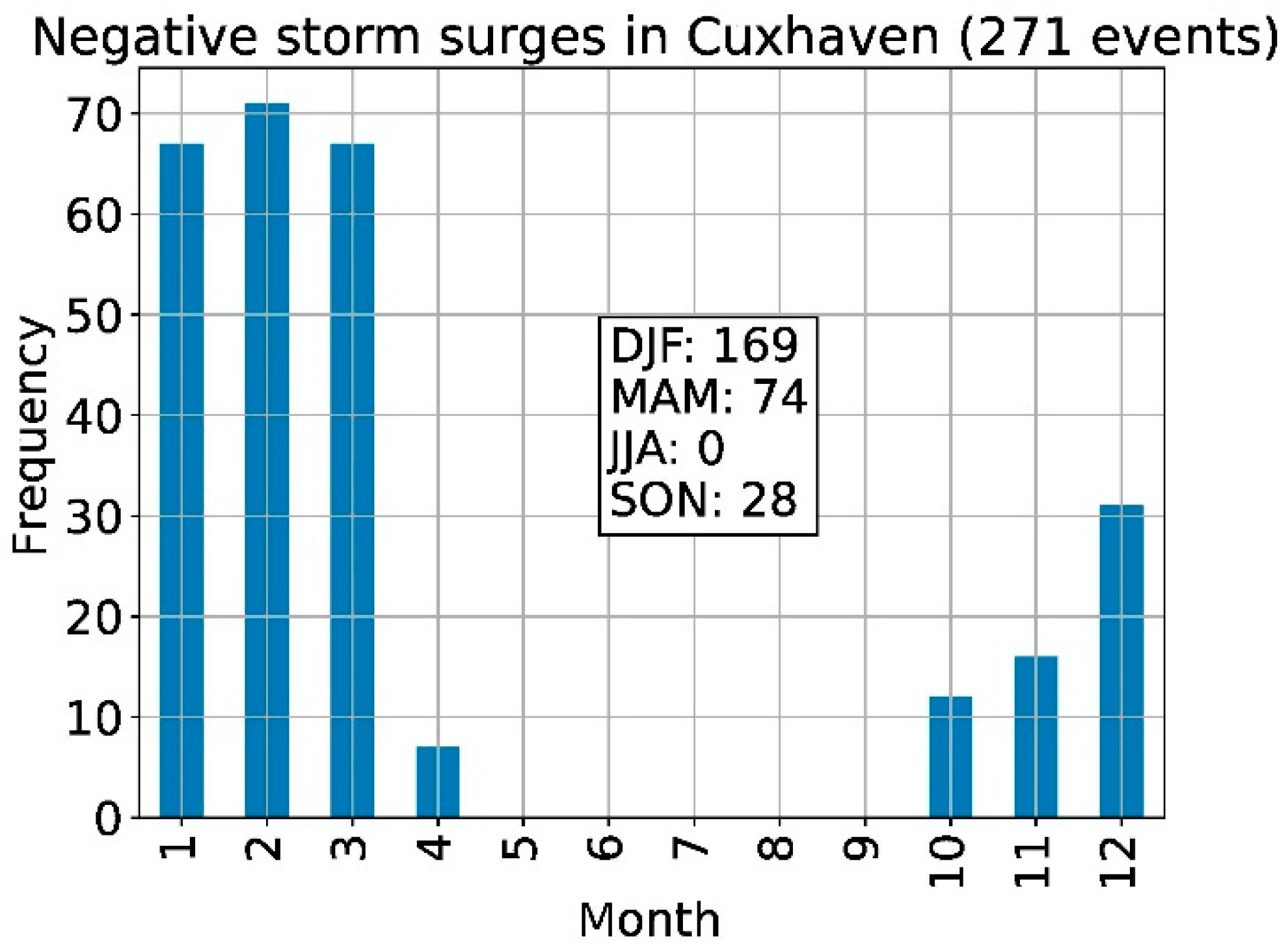
3.3. Timeseries of Extreme Low Water Events at Cuxhaven

Based on the definition given in Section 2.2.1, we identified 271 ELWs for Cuxhaven and the period 1950–2019 (see Figure 5). The number of ELWs as depicted in Figure 5 is characterized by high interannual variability; there is no statistically significant trend in the observation period.
Figure 6 shows the monthly distribution of the 271 ELWs. All 271 ELWs occurred between October and April, most of them in January, February and March. This is in line with expectations as winter and early spring are usually marked with higher synoptic variability in the atmosphere which is a pronounced succession of comparably stronger high and low pressure systems.

3.4. Mean Conditions before Negative Storm Tides

In the following, we analyse the climatology of the 271 ELWs that have been recorded between 1950 and 2019 at Cuxhaven. The aim is to identify typical situations, initiating the onset and/or prevailing during ELW events.

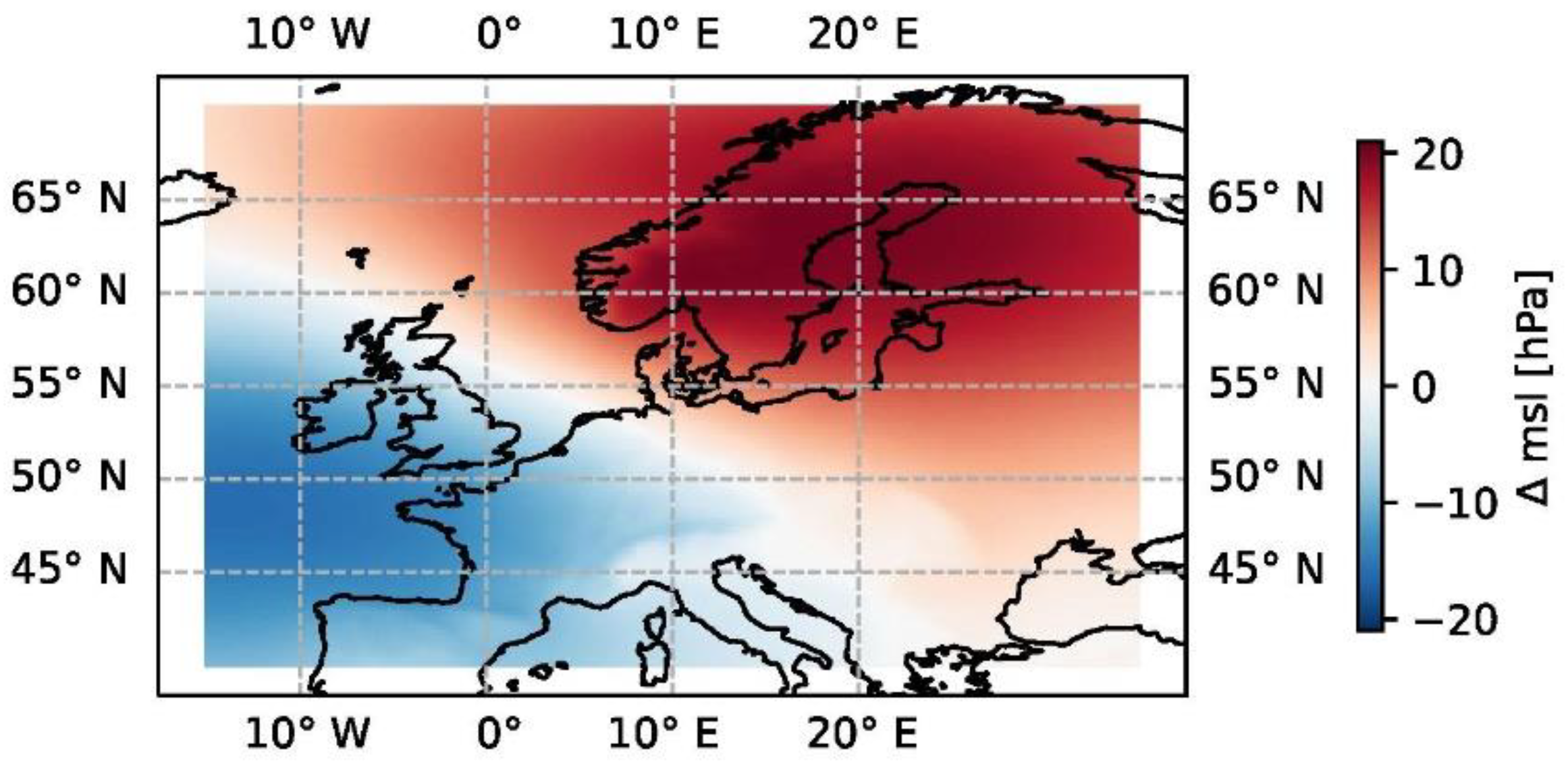
3.4.1. Pressure Field before Negative Storm Tide

A first overview regarding the meteorological conditions right before the 271 ELWs is provided by the SLP composite anomaly: Figure 7 shows the mean anomaly of the mean pressure fields 24 h before all 271 events, based on the climatology of 1971–2000. This composite is marked by a dipolar pattern separated along the north-west to south-east axis, with a positive pressure anomaly over Scandinavia and a negative pressure anomaly over the north Atlantic and the Iberian Peninsula. This pattern is very similar to the pattern for anomalies for all days classified as LWT SE (independent of the occurrence of an ELW; see Figure 8) but shows stronger anomalies. It also matches the situation seen in the case study of 2018 (see Section 3.2) and corresponds well with the effective wind direction of 142° (see Section 2.2.4) that was derived for ELWs at Cuxhaven.

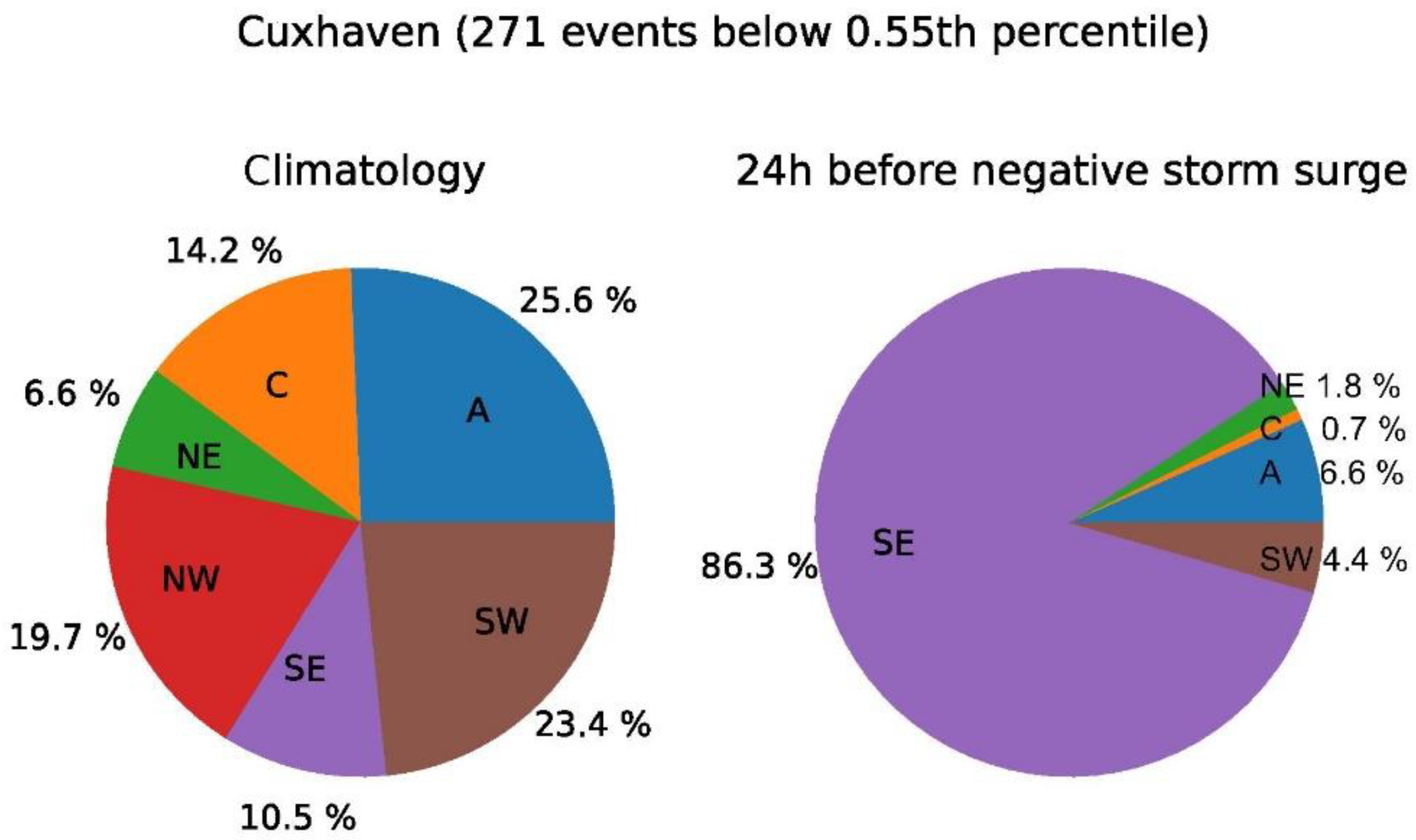
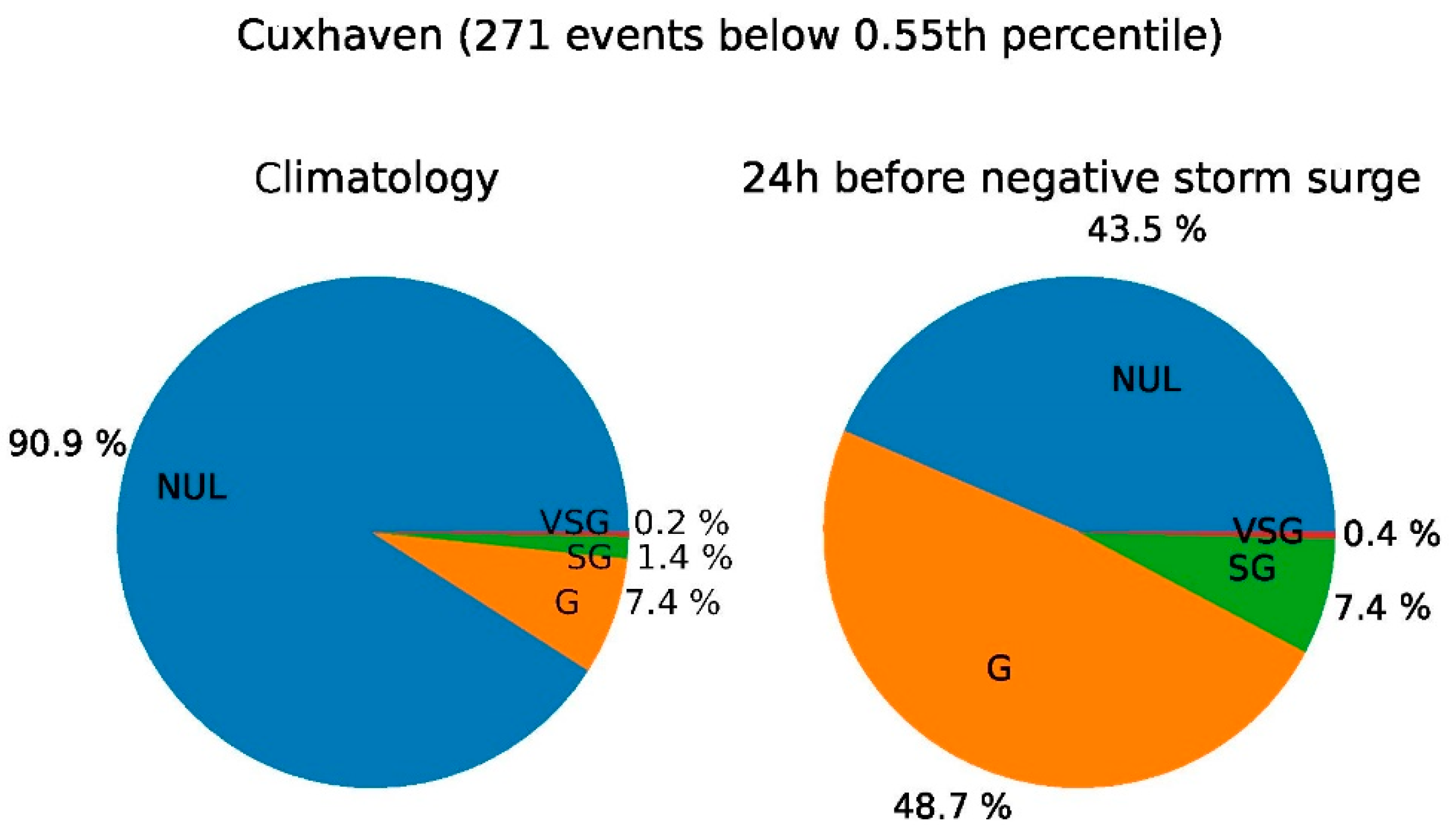
3.4.2. Weather Types

Figure 9 shows the relative frequencies of the LWT (Section 2.2.2) calculated from daily ERA5 SLP data over the entire period (1950–2019) independent of the occurrence of ELWs (left), as well as for the 24 h before the ELW (right).
While a south-east weather type (SE) occurs climatologically with a probability of 10.5%, it occurs with a probability of 86.3% directly before an ELW. Therefore, an SE LWT is 8 times more likely at the onset of such an event. This difference is statistically highly significant (p < 0.001; tested via 10,000-fold bootstrapping). For the other LWTs, this probability decreases proportionally: LWTs with northerly winds (NW, NE) are hardly found (0 and 0.7 %, respectively) preceding ELWs. This finding confirms our geoscientific expectation since south-easterly winds can be regarded as offshore for the area around Cuxhaven.

3.4.3. Gale Strength

Similar to Figure 9, Figure 10 shows the distributions of gale strength derived from the LAMB weather classification based on daily ERA5 data over the entire period 1950–2019 (left), as well as for the 24 h before the ELW (right).
While a storm (G, SG and VSG) occurs on average with a probability of about 9%, it occurs with a probability of about 56.5% during the 24 h before an ELW. This significant difference (p < 0.001 tested via 10,000-fold bootstrapping) confirms the expectation that comparatively high wind speeds on a larger spatial scale are necessary to produce ELWs.

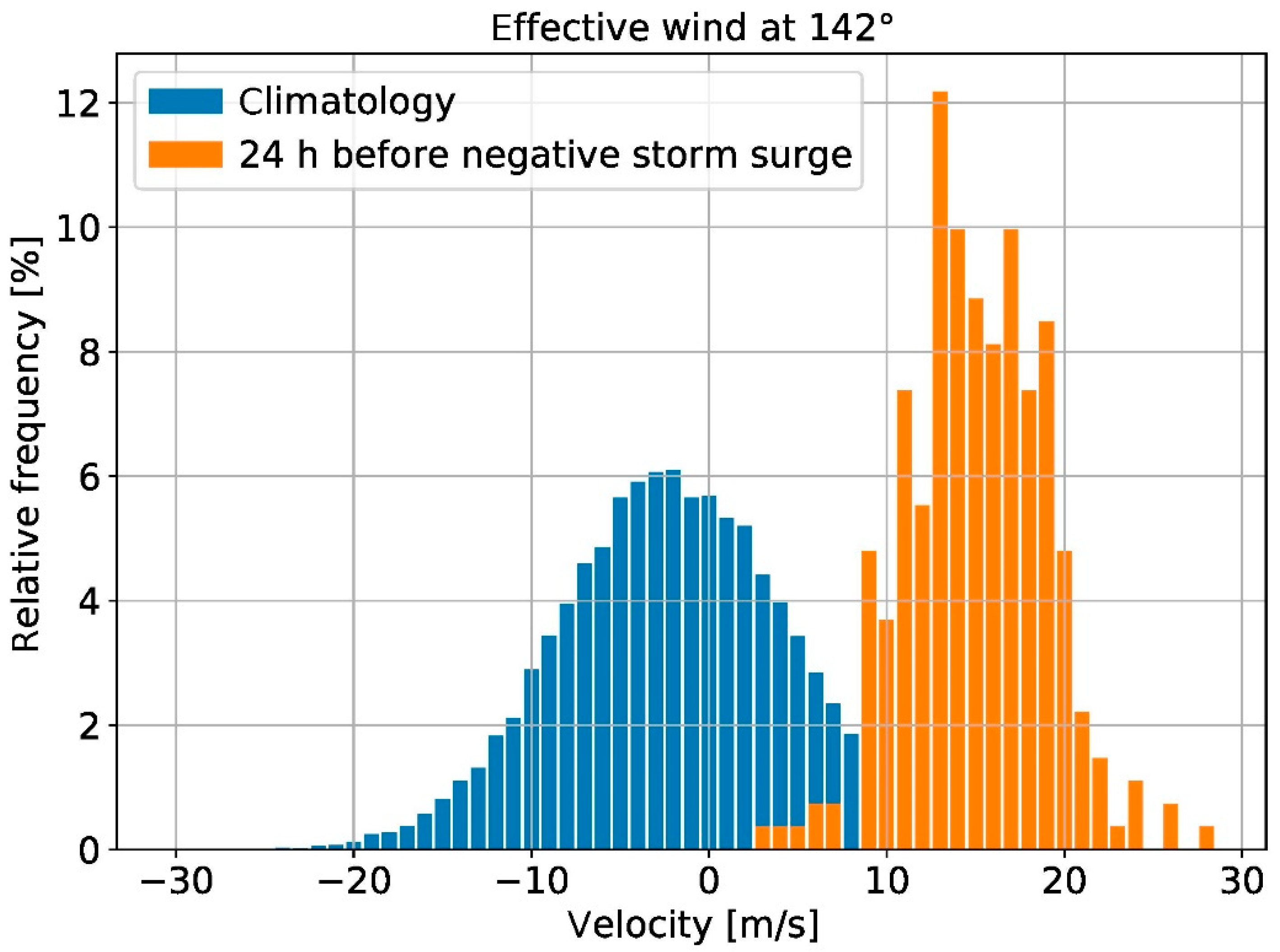
3.4.4. Effective Wind

Figure 11 shows the empirical probability distribution function of the effective wind (Section 2.2.4.) as a climatology of the daily mean for the entire period 1950–2019 and for the 24 h before ELWs. A clear distinction between the two distributions is obvious. Before ELWs, the effective wind was always positive and in more than 90% of all cases higher than 10 m/s which in turn approx. matches the 95th percentile of the climatological distribution. The mean of the ELW-sample is 15.6 m/s, while the climatological probability distribution of the effective wind spreads from about −30 m/s to 20 m/s with a mean value of approx. −2 m/s. The difference between these two mean values is statistically significant with p < 0.001 (based on 10,000-fold bootstrapping).

3.5. Future Scenarios

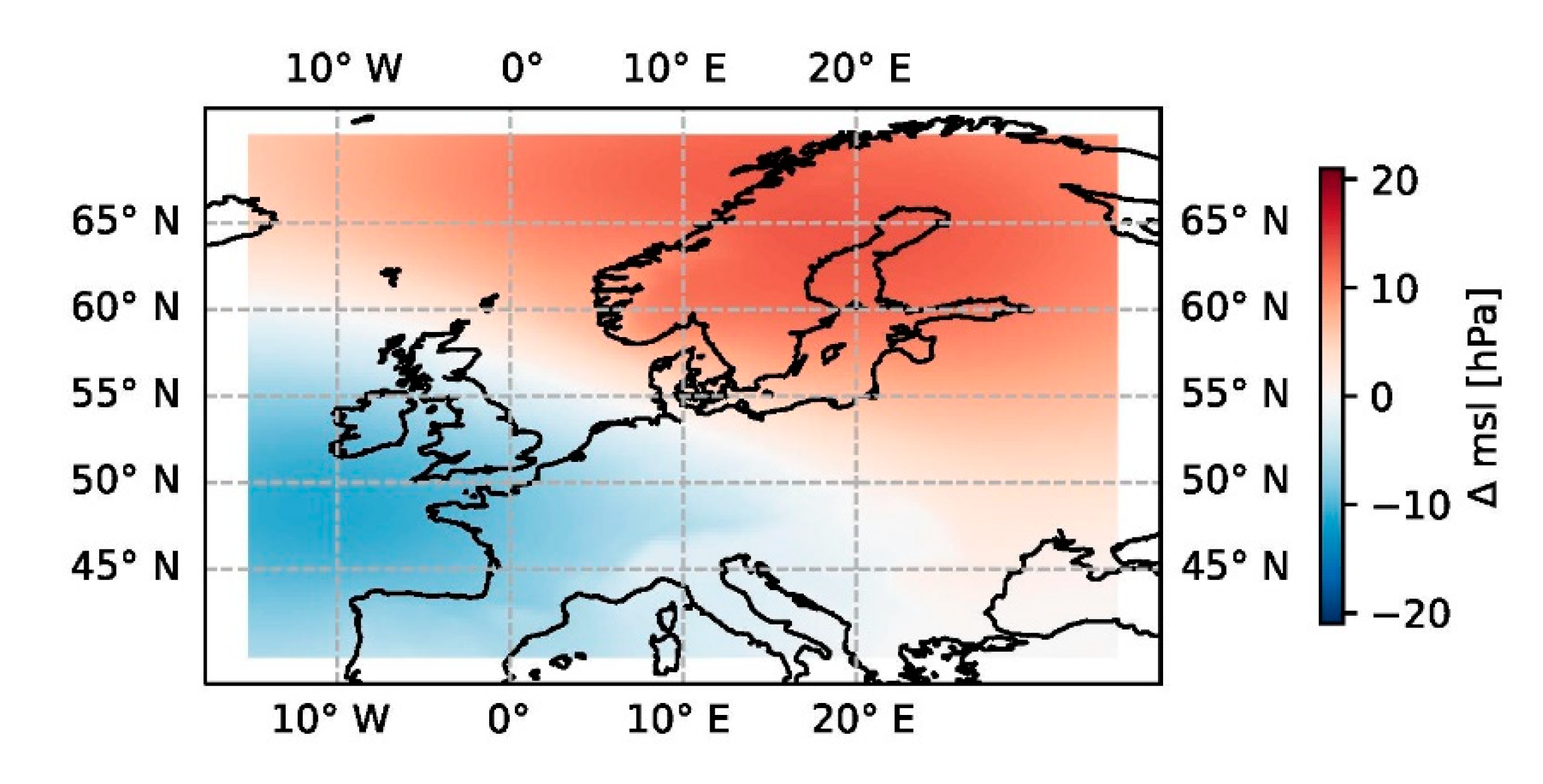
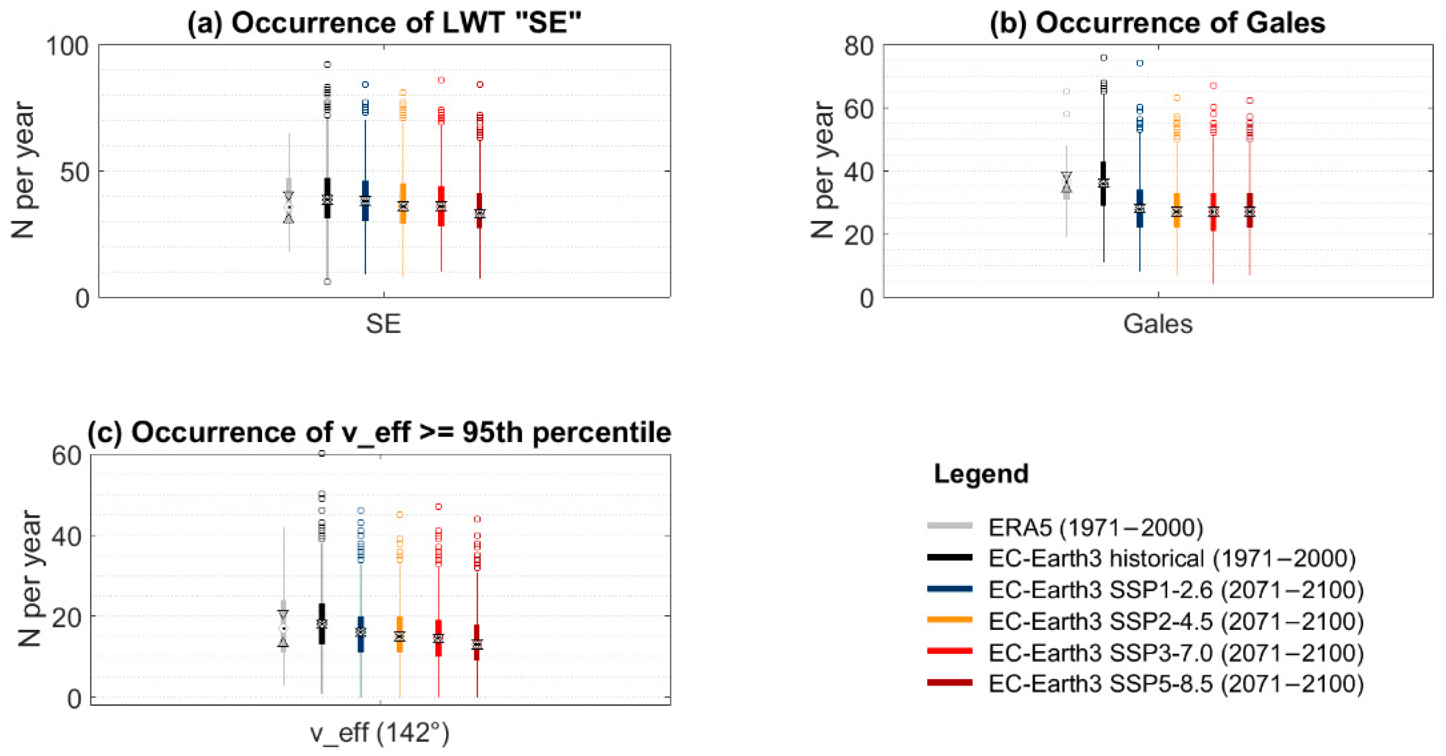
3.5.1. Future Development of Meteorological Conditions

Results from the previous sections show that both, wind direction (from Southeast) and wind speed are important to trigger ELWs. The question arises of whether these conditions might change in the future. We tackle this question by analysing the frequency of SE weather types, gale classes, as well as effective wind in four climate scenarios based on SMHI-LENS.
Figure 12a shows the distribution of the occurrence of the derived LWT “SE” per year for ERA5 and the 50-member SMHI-LENS ensemble for the historical period (1971–2000) and the far future (2071–2100) in SSP1-2.6, SSP2-4.5, SSP3-7.0, and SSP5-8.5, respectively. In these plots, two medians are significantly different (p < 0.05) if their confidence intervals (triangular markers) do not overlap. Therefore, it can be concluded that SMHI-LENS historical is consistent with ERA5 regarding the median frequency for the LWT “SE”. With climate change according to SMHI-LENS, the frequency of LWT SE systematically shifts towards lower values, with SSP5-8.5 being significantly (p < 0.05) lower than the historical equivalent.
Figure 12b shows the distribution of the occurrence of gales (G, SG, and VSG) per year for ERA5 and SMHI-LENS again for the historical period (1971–2000) and the far future (2071–2100). A significant decrease for all scenarios is apparent, while the inter-scenario differences are considerably smaller. While the “drop” in gales might seem strong, investigations of near future time-slices (2015–2044/2041–2070) reveal smaller decreases. In fact, the decrease already emerges towards the end of the historical period (1985–2014; not shown).
Figure 12c finally shows the distribution of the occurrence of effective winds being above the 95th percentile of the climatological probability distribution function of the historical period. In ERA5, this 95th percentile approximately matches the value of 10 m/s and we have seen in Figure 11 that the majority of ELWs were subject to effective winds beyond this threshold. Hence, we consider such extreme effective winds a reasonable proxy for the risk of ELWs, not taking into account any actual tide phases of course. The result is very much in line with what has been shown for the SE LWT as well as the gale strength already. SMHI-LENS shows a systematic shift towards less frequent situations with extreme effective winds under climate change. The stronger the climate change scenario, the lower the frequency of extreme effective winds, SSP2-4.5, SSP3-7.0, and SSP5-8.5 being significantly different from the historical experiment regarding the median frequency.

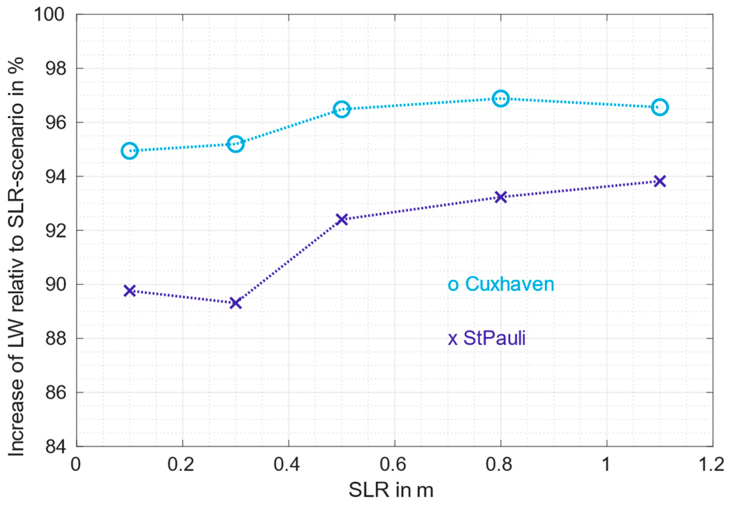
3.5.2. Influence of Future SLR on Negative Storm Tide Water Levels

The focus of this study lies on the meteorological conditions associated with ELW. However, SLR will become a non-negligible factor in this respect under continued global warming. Therefore, we include a sensitivity study based on the ELW event in March 2018 (marked by a star in Figure 3) and hydrodynamic modelling of different SLR scenarios for this particular event. The results are shown in Figure 13. It indicates, to which amount the lowest LW would rise at Cuxhaven and St. Pauli solely due to SLR. This is displayed as the relative increase, i.e., the rise of ELW due to SLR, scaled by SLR. That means, e.g., for the leftmost data point in Figure 13, that the 2018 event is subject to an SLR of 0.1 m would yield an approx. 0.09 m higher water level in St. Pauli. The relative increase is slightly higher in Cuxhaven than in St. Pauli. At both locations and for all simulated scenarios the increase lies between 88 and 98% of SLR.

4. Discussion

4.1. Development of Past LWs in the Elbe Estuary

Observations of LWs in the Elbe estuary since 1963 show a strongly decreasing trend for the median LW levels at St. Pauli and a slightly increasing trend for Cuxhaven. The minimum LW of each year, which is most likely strongly influenced by wind, shows a related decreasing and increasing trend for the two stations. The increase of LWs at Cuxhaven is very likely to be mainly caused by past sea level rise. According to [14] global mean SLR between 1971 and 2018 was in a likely range of 1.55 and 3.12 mm/a. For Cuxhaven, a regional mean SLR of 3.6 ± 0.8 mm/a between 1971 and 2008 was calculated by [57]. At St. Pauli the observed LW is still influenced by varying discharge into the estuary. The decreasing trend of LWs at St. Pauli can be caused by the anthropogenic changes in the estuary geometry [58], as well as morphological changes and low discharge volumes [59]. These changes seem to have outweighed the effect of sea level rise at St. Pauli in the past.

4.2. Favouring Meteorological Conditions

Our results show, that there is a strong connection between the general direction of the atmospheric circulation and a potential for an ELW. Some studies already showed that the remote winds play an important role in more exposed locations [4,7]. Analysis based on an objective weather classification scheme showed that the SE weather type and an effective wind direction of 142° both mark situations where the wind is blowing offshore, literally pushing the water out of the Elbe estuary. Most (>85%) of the ELWs coincide with a SE weather type which is a frequency that is significantly higher than expected from climatology (10.5%; p < 0.001). In addition, the wind magnitude, in our case represented by distinct gale classes, was considered. Over half (>55%) of the events were preceded by a wind field classified as a storm for the North Sea area, again significantly more frequent than expected from climatology (9.1%, p < 0.001). The effective wind is combining the direction and the strength of the flow and with >90% of the events with prevailing effective wind above 10 m/s. This is a strongly favouring condition for ELWs in the Elbe estuary.
The small p-values found for these differences from climatology indicate that the statistical likelihood of the findings resulting from chance is very low. However, the specific numbers are of course subject to a few uncertainties. These are mainly based on the dataset used and the employed weather type classification scheme. Usage of other pressure data and/or a different classification scheme will yield slightly differing numbers. To our knowledge, there is no previous research done on ELWs in the German bight and the Elbe estuary. However, the results confirm what would be expected for the location of the Elbe estuary: Considering the overall geographic situation and coastline of the German Bight as well as the well-known fact that north-westerly winds are associated with (positive) storm tides on the German North Sea coast (see, e.g., [45]) it was expected that a contrasting south-easterly wind would lead to ELWs.
The meteorological analysis in this study is solely based on large-scale conditions that are derived from SLP data. Further analysis of gridded wind fields or direct wind measurements before and during ELWs could possibly extend the knowledge of the effect of local wind on these extreme water levels.

4.3. Possible Future Changes in Favouring Meteorological Conditions

For the investigation of possible future changes, SMHI-LENS—a large ensemble of the GCM EC-Earth3—was used. While the exploitation of this large ensemble of 50 members significantly reduces the uncertainty of climate change signal estimates, the problem of model uncertainty prevails. The results presented here show a clear signal that conditions leading to ELWs will become significantly less frequent, especially when considering scenarios of strong global warming. However, similar investigations with different GCMs may yield differing outcomes. A profound multi-model analysis would yield a more robust assessment in this respect.

4.4. Effect of Future Sea Level Rise on ELWs

To estimate the effect of future SLR on ELWs, the ELW chain event from March 2018 was simulated with a hydrodynamic-numerical model, applying different SLR scenarios. A comparison shows that the observed water level during the ELW chain event 2018 is well reproduced by the model. The results show an increase of the lowest LW at Cuxhaven and St. Pauli between 88 and 98% relative to the SLR scenarios of 10, 30, 50, 80 and 110 cm. The weaker increase of ELW at St. Pauli compared to Cuxhaven results from the stronger increase of tidal range due to SLR at St. Pauli. A detailed study on the influence of SLR on tidal amplification in the Elbe estuary is currently in process. To our knowledge, there are no previous studies on the influence of SLR on ELWs in the Elbe estuary. However, studies on the effect of SLR on mean tides [19] and (positive) storm surges [18] in the Elbe estuary revealed a similarly strong influence of SLR on the water levels along the estuary including the station St. Pauli, as we observed for the ELW 2018. NSS and resulting ELWs occur as a result of the interaction between astronomical tide and meteorological conditions and are therefore individual in their characteristics. Nevertheless, it can be assumed, that the possible influence of future SLR on other ELW events in the Elbe estuary is in the same order of magnitude, as the essential interactions of involved driving forces remain the same. It should be noted, that all simulation results were derived with reference topography in the Elbe estuary from the year 2019. The effect of possible future changes of estuary topography are therefore not included in the displayed results. As discussed for the development of LW observations in the Elbe estuary, topographic changes strongly influenced LWs at St. Pauli in the past. It can be assumed, that tidal flats in the Wadden Sea will grow to a certain amount with sea level rise, as they did in the past [60], because coastal topography and tidal dynamics strive towards a morphodynamic equilibrium [61]. However, future morphologic changes in the context of climate change and accelerated SLR, as well as anthropogenic measures in the Elbe estuary are difficult to estimate. Therefore, reliable predictions of future topography in the Elbe estuary are not available based on today’s knowledge and further investigation in this regard is needed.

5. Conclusions and Outlook

This article investigated the impact of large-scale meteorological conditions as well as changing sea levels on ELWs in the Elbe estuary.
Different parameters were considered in the 24 h preceding an ELW at the gauge in Cuxhaven in order to analyse which atmospheric conditions (weather type, storminess and effective wind) prevail before such an extreme event. The investigations show that the SE weather type is represented 8 times more frequently before an ELW than it would be expected climatologically. Effective wind speeds (wind direction of 142°) with more than 10 m/s occur 17 times more frequently than expected from climatology.
Furthermore, possible future changes in these parameters were analysed using a single-model large ensemble of the GCM simulations with 4 different future scenarios. All three previously considered parameters show a significant decrease in the frequency of conditions favourable for ELWs for the far future (2071–2100), especially in the highest emission scenario SSP5-8.5.
In addition to changing atmospheric conditions, future ELWs in the Elbe estuary will be influenced by SLR: Projections for future SLR are varying for the different SSP-scenarios within a range of 51 and 85 cm for the median at Cuxhaven for the year 2100 relative to the reference period 1995–2014 [14,15,16]. Our simulation results indicate, how different SLR scenarios would increase the lowest ELW in March 2018. At the locations Cuxhaven and St. Pauli the increase lies between 88 and 98% of the simulated SLR scenarios of 10, 30, 50, 80 and 110 cm. It can be assumed, that the possible influence of future SLR on ELW events in the Elbe estuary is in the same order of magnitude as determined for the ELW 2018. SLR will therefore lead to less extreme and fewer ELWs in the future.
Therefore, our study suggests that both SLR and meteorological conditions in a warmer future climate will be less favourable for the occurrence of ELWs in the Elbe estuary, but—if they occur—can be associated with significant negative effects on shipping transport towards the Port of Hamburg as well as certain waterfront structures.
These results for potential future changes should and will be reviewed based on the extended analysis of a multi-model ensemble in order to account for the existing model uncertainty. Nevertheless, the prospect of a potential decrease in ELWs due to both—less favourable meteorological conditions and SLR—raises the question whether (positive) storm tides in contrast might increase in strength or frequency in the future. Even though this topic is much better covered by existing studies, further investigations in this respect based on the most recent generation of climate models and future scenarios are desired.

Author Contributions

Conceptualization, C.J., T.M. and T.K.; methodology, C.J. and T.M.; validation, T.M.; investigation, C.J., T.M. and N.H.S.; writing—original draft preparation, C.J., T.M., N.H.S. and T.K.; writing—review and editing, C.J., T.M., N.H.S., I.H. and T.K; visualization, C.J., T.M. and N.H.S.; supervision, T.K. All authors have read and agreed to the published version of the manuscript.

Funding

This study was funded by the German Federal Ministry of Digital and Transport (BMDV) in the context of the BMDV Network of Experts.

Data Availability Statement

Tidal low water observations at Cuxhaven:Measured by WSA (Waterways and Shipping Agency) Elbe-North sea. Available at [29]. Tidal low water observations at St. Pauli: Measured by Hamburg Port Authority (HPA) Available at [29]. ERA5 SLP data: The ERA5-SLP data is publically available from the Copernicus Climate Change Service (C3S) Climate Data Store (CDS). Hersbach, H., Bell, B., Berrisford, P., Biavati, G., Horányi, A., Muñoz Sabater, J., Nicolas, J., Peubey, C., Radu, R., Rozum, I., Schepers, D., Simmons, A., Soci, C., Dee, D., Thépaut, J-N. (2018): ERA5 hourly data on single levels from 1979 to present. Copernicus Climate Change Service (C3S) Climate Data Store (CDS). (accessed on 13 June 2022), DOI: 10.24381/cds.adbb2d47; SMHI-LENS SLP data: The daily mean SLP-fields of SMHI-LENS are publically available from the Earth System Grid Federations (ESGF) as ensemble members r101-r150 for the respective experiments. EC-Earth Consortium (2019): EC-Earth-Consortium EC-Earth3 model output prepared for CMIP6 CMIP historical. Version 20200412.Earth System Grid Federation. https://doi.org/10.22033/ESGF/CMIP6.4700; EC-Earth Consortium (2019): EC-Earth-Consortium EC-Earth3 model output prepared for CMIP6 CMIP ssp126. Version 20210615.Earth System Grid Federation. https://doi.org/10.22033/ESGF/CMIP6.4874; EC-Earth Consortium (2019): EC-Earth-Consortium EC-Earth3 model output prepared for CMIP6 CMIP ssp245. Version 20210401.Earth System Grid Federation. https://doi.org/10.22033/ESGF/CMIP6.4880; EC-Earth Consortium (2019): EC-Earth-Consortium EC-Earth3 model output prepared for CMIP6 CMIP ssp370. Version 20210101.Earth System Grid Federation. https://doi.org/10.22033/ESGF/CMIP6.4884; EC-Earth Consortium (2019): EC-Earth-Consortium EC-Earth3 model output prepared for CMIP6 CMIP ssp585. Version 20200412.Earth System Grid Federation. https://doi.org/10.22033/ESGF/CMIP6.4912Di charge observations at Neu Darchau: Measured by WSA (Waterways and Shipping Agency) Elbe. Available at the Coastal Data Portal of the WSV (Federal Waterways and Shipping Administration) https://www.kuestendaten.de/DE/dynamisch/appl/data/daten_prod/prodNeuProd/direct_download/ab_darchau!Abfluss.zip. The data was last downloaded in June 2021.Water level Observations at Cuxhaven:Measured by WSA (Waterways and Shipping Agency) Elbe-Nordsee. Available at the Coastal Data Portal of the WSV (Federal Waterways and Shipping Administration) https://www.kuestendaten.de/DE/dynamisch/appl/data/daten_prod/prodNeuProd/direct_download/cuxhaven_steubenhoeft!Wasserstand_(NN-Bezug).zip. The data was last downloaded in June 2021.Observation of wind velocity and direction at Scharhörn: Measured by Hamburg Port Authority (HPA).Available at the Coastal Data Portal of the WSV (Federal Waterways and Shipping Administration). https://www.kuestendaten.de/DE/dynamisch/appl/data/daten_prod/prodNeuProd/direct_download/HPA_Meteo_Scharhoern!Windgeschwindigkeit.zip. The data was last downloaded in June 2021. COSMOREA6: The data is generated and made available by the Hans Ertel Center of the University of Bonn in cooperation with the DWD (Deutscher Wetterdienst) (https://reanalysis.meteo.uni-bonn.de/?COSMO-REA6___Specifications). Available at: https://opendata.dwd.de/climate_environment/REA/COSMO_REA6/. The data was last downloaded in June 2021. Bathymetrie year 2016. The Data was generated by the EasyGSH-ProjectAvailable at: https://mdi-de.baw.de/easygsh/EasyEN_DownloadG.html#2016. Last checked: June 2021.

Conflicts of Interest

The authors declare no conflict of interest.

Appendix A

Figure A1. Distribution of the U and V components of the geostrophic wind from the LWT classification for daily means (black) and for the 24-h mean before an ELW (red). Marked also is whether a gale was present at that time (blue and yellow ‘x’, respectively).
Atmosphere 13 01634 g0a1
Figure A2. Water level at several stations during the negative storm surge event 2018; observation (black) and simulation result (red).
Atmosphere 13 01634 g0a2aAtmosphere 13 01634 g0a2b

References

  1. HTG. Empfehlungen des Arbeitsausschusses “Ufereinfassungen” Häfen und Wasserstraßen EAU 2020: (inkl. E-Book als PDF), 12th ed.; Ernst Wilhelm & Sohn: Berlin, Germany, 2020. [Google Scholar]
  2. Port of Hamburg “Seaborne Cargo Handling”. Available online: https://www.hafen-hamburg.de/en/statistics/seabornecargohandling/ (accessed on 25 April 2022).
  3. Hamburg Port Authority. Gewässerkundliche Information—Gewässerkundliches Jahr 2019—Pegel St. Pauli: 1 November 2018–31 October 2019. Available online: https://www.hamburg-port-authority.de/fileadmin/user_upload/Gewaesserkundliche_Information_2019.pdf (accessed on 9 June 2022).
  4. Gurumurthy, P.; Orton, P.M.; Talke, S.A.; Georgas, N.; Booth, J.F. Mechanics and Historical Evolution of Sea Level Blowouts in New York Harbor. JMSE 2019, 7, 160. [Google Scholar] [CrossRef] [Green Version]
  5. Gönnert, G.; Dube, S.K.; Murty, T.; Siefert, W. 7. Storm Surges generated by Extra-Tropical Cyclones—Case Studies. Die Küste—Sonderh. Glob. Storm Surges 2001, 63, 455–546. [Google Scholar]
  6. Sztobryn, M.; Weidig, B.; Stanislawczyk, I. Niedrigwasser in der Südlichen Ostsee (Westlicher und Mittlerer Teil); Bundesamt für Seeschifffahrt und Hydrographie: Hamburg, Germany, 2009; Volume 45.
  7. Campetella, C.M.; D’Onofrio, E.; Cerne, S.B.; Fiore, M.E.; Possia, N.E. Negative storm surges in the port of Buenos Aires. Int. J. Climatol. 2007, 27, 1091–1101. [Google Scholar] [CrossRef]
  8. Wicks, A.J.; Atkinson, D.E. Identification and classification of storm surge events at Red Dog Dock, Alaska, 2004–2014. Nat. Hazards 2016, 86, 877–900. [Google Scholar] [CrossRef]
  9. Wolski, T.; Wiśniewski, B. Geographical diversity in the occurrence of extreme sea levels on the coasts of the Baltic Sea. J. Sea Res. 2020, 159, 101890. [Google Scholar] [CrossRef]
  10. Geelhoed, P. Negative Surges in the Southern North Sea. Int. Hydrogr. Rev. 1973, 61–73. [Google Scholar]
  11. Conte, D.; Lionello, P. Characteristics of large positive and negative surges in the Mediterranean Sea and their attenuation in future climate scenarios. Glob. Planet. Change 2013, 111, 159–173. [Google Scholar] [CrossRef]
  12. Pugh, D.; Woodworth, P. Sea-Level Science: Understanding Tides, Surges, Tsunamis and Mean Sea-Level Changes; Cambridge University Press: Cambridge, UK, 2014. [Google Scholar]
  13. Booth, J.F.; Narinesingh, V.; Towey, K.L.; Jeyaratnam, J. Storm Surge, Blocking, and Cyclones: A Compound Hazards Analysis for the Northeast United States. J. Appl. Meteorol. Climatol. 2021, 60, 1531–1544. [Google Scholar] [CrossRef]
  14. Fox-Kemper, B.; Hewitt, H.T.; Xiao, C.; Aðalgeirsdóttir, G.; Drijfhout, S.S.; Edwards, T.L.; Golledge, N.R.; Hemer, M.; Kopp, R.E.; Krinner, G.; et al. Ocean, Cryosphere and Sea Level Change. In Climate Change 2021: The Physical Science Basis. Contribution of Working Group I to the Sixth Assessment Report of the Intergovernmental Panel on Climate Change; Cambridge University Press: Cambridge, UK, 2021; Volume 6, pp. S.1211–S.1362. [Google Scholar] [CrossRef]
  15. Garner, G.G.; Kopp, R.E.; Hermans, T.; Slangen, A.B.A.; Koubbe, G.; Turilli, M.; Jha, S.; Edwards, T.L.; Levermann, A.; Nowikci, S.; et al. Framework for Assessing Changes to Sea-level (FACTS). Geosci. Model Dev. 2021. in prep.. [Google Scholar]
  16. Garner, G.G.; Hermans, T.; Kopp, R.E.; Slangen, A.B.A.; Edwards, T.L.; Levermann, A.; Nowikci, S.; Palmer, M.D.; Smith, C.; Fox-Kemper, B.; et al. IPCC AR6 Sea-Level Rise Projections. Version 20210809. Available online: https://podaac.jpl.nasa.gov/announcements/2021-08-09-Sea-level-projections-from-the-IPCC-6th-Assessment-Report (accessed on 16 May 2022).
  17. Khojasteh, D.; Glamore, W.; Heimhuber, V.; Felder, S. Sea level rise impacts on estuarine dynamics: A review. Sci. Total Environ. 2021, 780, 146470. [Google Scholar] [CrossRef]
  18. Rudolph, E. Storm Surges in the Elbe, Jade-Weser and Ems Estuaries. Die Küste 2014, 81, 291–300. [Google Scholar]
  19. Seiffert, R.; Hesser, F. Investigating Climate Change Impacts and Adaptation Strategies in German Estuaries. Die Küste 2014, 81, 551–563. [Google Scholar]
  20. Kučerová, M.; Beck, C.; Philipp, A.; Huth, R. Trends in frequency and persistence of atmospheric circulation types over Europe derived from a multitude of classifications. Int. J. Climatol. 2017, 37, 2502–2521. [Google Scholar] [CrossRef]
  21. Stryhal, J.; Huth, R. Trends in winter circulation over the British Isles and central Europe in twenty-first century projections by 25 CMIP5 GCMs. Clim. Dyn. 2018, 52, 1063–1075. [Google Scholar] [CrossRef]
  22. Huguenin, M.F.; Fischer, E.M.; Kotlarski, S.; Scherrer, S.C.; Schwierz, C.; Knutti, R. Lack of Change in the Projected Frequency and Persistence of Atmospheric Circulation Types Over Central Europe. Geophys. Res. Lett. 2020, 47, e2019GL086132. [Google Scholar] [CrossRef]
  23. Donat, M.G.; Leckebusch, G.C.; Pinto, J.G.; Ulbrich, U. European storminess and associated circulation weather types: Future changes deduced from a multi-model ensemble of GCM simulations. Clim. Res. 2010, 42, 27–43. [Google Scholar] [CrossRef]
  24. Plavcová, E.; Kyselý, J. Projected evolution of circulation types and their temperatures over Central Europe in climate models. Theor. Appl. Climatol. 2013, 114, 625–634. [Google Scholar] [CrossRef]
  25. Riediger, U.; Gratzki, A. Future weather types and their influence on mean and extreme climate indices for precipitation and temperature in Central Europe. Meteorol. Z. 2014, 23, 231–252. [Google Scholar] [CrossRef]
  26. Demuzere, M.; Werner, M.; van Lipzig, N.P.M.; Roeckner, E. An analysis of present and future ECHAM5 pressure fields using a classification of circulation patterns. Int. J. Climatol. 2009, 29, 1796–1810. [Google Scholar] [CrossRef] [Green Version]
  27. Arns, A.; Wahl, T.; Dangendorf, S.; Jensen, J. The impact of sea level rise on storm surge water levels in the northern part of the German Bight. Coast. Eng. 2015, 96, 118–131. [Google Scholar] [CrossRef]
  28. Müller-Navarra, S.H.; Giese, H. Improvements of an empirical model to forecast wind surge in the German Bight. Ocean Dyn. 1999, 51, 385–405. [Google Scholar] [CrossRef]
  29. WSV. Zentrales Datenmanagement (ZDM): Küstendaten. Available online: https://www.kuestendaten.de/DE/Services/Messreihen_Dateien_Download/Download_Zeitreihen_node.html (accessed on 9 June 2022).
  30. Hersbach, H.; Bell, B.; Berrisford, P.; Hirahara, S.; Horányi, A.; Muñoz-Sabater, J.; Nicolas, J.; Peubey, C.; Radu, R.; Schepers, D. The ERA5 global reanalysis. Q. J. R. Meteorol. Soc. 2020, 146, 1999–2049. [Google Scholar] [CrossRef]
  31. ECMWF. ERA5. Available online: https://confluence.ecmwf.int/display/CKB/ERA5 (accessed on 12 August 2021).
  32. Bell, B.; Hersbach, H.; Simmons, A.; Berrisford, P.; Dahlgren, P.; Horányi, A.; Muñoz-Sabater, J.; Nicolas, J.; Radu, R.; Schepers, D.; et al. The ERA5 global reanalysis: Preliminary extension to 1950. Q. J. R. Meteorol. Soc. 2021, 147, 4186–4227. [Google Scholar] [CrossRef]
  33. Schade, N.H.; Sadikni, R.; Jahnke-Bornemann, A.; Hinrichs, I.; Gates, L.; Tinz, B.; Stammer, D. The KLIWAS North Sea climatology. Part II: Assessment against global reanalyses. J. Atmos. Ocean. Technol. 2017, 35, 127–145. [Google Scholar] [CrossRef]
  34. Wyser, K.; Koenigk, T.; Fladrich, U.; Fuentes-Franco, R.; Karami, M.P.; Kruschke, T. The SMHI Large Ensemble (SMHI-LENS) with EC-Earth3.3.1. Geosci. Model Dev. 2021, 14, 4781–4796. [Google Scholar] [CrossRef]
  35. Döscher, R.; Acosta, M.; Alessandri, A.; Anthoni, P.; Arsouze, T.; Bergman, T.; Bernardello, R.; Boussetta, S.; Caron, L.-P.; Carver, G.; et al. The EC-Earth3 Earth system model for the Coupled Model Intercomparison Project 6. Geosci. Model Dev. 2022, 15, 2973–3020. [Google Scholar] [CrossRef]
  36. Eyring, V.; Bony, S.; Meehl, G.A.; Senior, C.A.; Stevens, B.; Stouffer, R.J.; Taylor, K.E. Overview of the Coupled Model Intercomparison Project Phase 6 (CMIP6) experimental design and organization. Geosci. Model Dev. 2016, 9, 1937–1958. [Google Scholar] [CrossRef] [Green Version]
  37. O’Neill, B.C.; Tebaldi, C.; van Vuuren, D.P.; Eyring, V.; Friedlingstein, P.; Hurtt, G.; Knutti, R.; Kriegler, E.; Lamarque, J.-F.; Lowe, J.; et al. The Scenario Model Intercomparison Project (ScenarioMIP) for CMIP6. Geosci. Model Dev. 2016, 9, 3461–3482. [Google Scholar] [CrossRef] [Green Version]
  38. Bundesamt für Seeschifffahrt und Hydrographie “Sturmfluten”. Available online: https://www.bsh.de/DE/THEMEN/Wasserstand_und_Gezeiten/Sturmfluten/sturmfluten_node.html (accessed on 12 May 2020).
  39. Gerber, M.; Ganske, A.; Müller-Navarra, S.; Rosenhagen, G. Categorisation of Meteorological Conditions for Storm Tide Episodes in the German Bight. Meteorol. Z. 2016, 25, 447–462. [Google Scholar] [CrossRef]
  40. Lamb, H.H. Types and spells of weather around the year in the British Isles: Annual trends, seasonal structure of the year, singularities. Q. J. R. Meteorol. Soc. 1950, 76, 393–429. [Google Scholar] [CrossRef]
  41. Jenkinson, A.F.; Collison, F.P. An initial climatology of gales over the North Sea. Synop. Climatol. Branch Memo. 1977, 62, 18. [Google Scholar]
  42. Loewe, P. Nordseezustand 2003; Bundesamt für Seeschifffahrt und Hydrographie: Hamburg/Rostock, Germany, 2005; Volume 38.
  43. Loewe, P. System Nordsee—Zustand 2005 im Kontext Langzeitlicher Entwicklungen; Bundesamt für Seeschifffahrt und Hydrographie: Hamburg/Rostock, Germany, 2009; Volume 44.
  44. Federal Agency for Cartography and Geodesy. 2021. Available online: https://sgx.geodatenzentrum.de/web_public/Datenquellen_TopPlusOpen_30.09.2021.pdf (accessed on 12 May 2020).
  45. Koziar, C.; Renner, V. MUSE Modellgestützte Untersuchungen zu Sturmfluten mit sehr geringen Eintrittswahrscheinlichkeiten–Teilprojekt: Numerische Berechnung physikalisch konsistenter Wetterlagen mit Atmosphärenmodellen; Deutscher Wetterdienst: Offenbach, Germany, 2005. [CrossRef]
  46. Ganske, A.; Fery, N.; Gaslikova, L.; Grabemann, I.; Weisse, R.; Tinz, B. Identification of extreme storm surges with high-impact potential along the German North Sea coastline. Ocean Dyn. 2018, 68, 1371–1382. [Google Scholar] [CrossRef]
  47. Casulli, V. A high-resolution wetting and drying algorithm for free-surface hydrodynamics. Int. J. Numer. Meth. Fluids 2009, 60, 391–408. [Google Scholar] [CrossRef]
  48. Smith, S.D.; Banke, E.G. Variation of the sea surface drag coefficient with wind speed. Q. J. R. Meteorol. Soc. 1975, 101, 665–673. [Google Scholar] [CrossRef]
  49. Sievers, J.; Malte, R.; Milbradt, P. EasyGSH-DB: Bathymetrie (1996–2016); Bundesanstalt für Wasserbau: Karlsruhe, Germany, 2020. [CrossRef]
  50. Bollmeyer, C.; Keller, J.D.; Ohlwein, C.; Wahl, S.; Crewell, S.; Friederichs, P.; Hense, A.; Keune, J.; Kneifel, S.; Pscheidt, I.; et al. Towards a high-resolution regional reanalysis for the European CORDEX domain. Q.J.R. Meteorol. Soc. 2015, 141, 1–15. [Google Scholar] [CrossRef]
  51. DWD. OPENDATA. Available online: https://opendata.dwd.de/climate_environment/REA/COSMO_REA6/ (accessed on 1 June 2022).
  52. Ganske, A.; Rosenhagen, G. Downscaling von Windfeldern aus Lokalmodellen auf die Tideelbe. Die Küste 2012, 79, 125–140. [Google Scholar]
  53. Borsche, M.; Kaiser-Weiss, A.K.; Kaspar, F. Wind speed variability between 10 and 116 m height from the regional reanalysis COSMO-REA6 compared to wind mast measurements over Northern Germany and the Netherlands. Adv. Sci. Res. 2016, 13, 151–161. [Google Scholar] [CrossRef] [Green Version]
  54. Zijl, F.; Verlaan, M.; Gerritsen, H. Improved water-level forecasting for the Northwest European Shelf and North Sea through direct modelling of tide, surge and non-linear interaction. Ocean Dyn. 2013, 63, 823–847. [Google Scholar] [CrossRef]
  55. Zijl, F.; Sumihar, J.; Verlaan, M. Application of data assimilation for improved operational water level forecasting on the northwest European shelf and North Sea. Ocean Dyn. 2015, 65, 1699–1716. [Google Scholar] [CrossRef] [Green Version]
  56. Rasquin, C.; Seiffert, R.; Wachler, B.; Winkel, N. The significance of coastal bathymetry representation for modelling the tidal response to mean sea level rise in the German Bight. Ocean Sci. 2020, 16, 31–44. [Google Scholar] [CrossRef] [Green Version]
  57. Wahl, T.; Jensen, J.; Frank, T.; Haigh, I.D. Improved estimates of mean sea level changes in the German Bight over the last 166 years. Ocean Dyn. 2011, 61, 701–715. [Google Scholar] [CrossRef]
  58. Siefert, W. Tiden und Sturmfluten in der Elbe und ihren Nebenflüssen: Die Entwicklung von 1950 bis 1997 und ihre Ursachen. Die Küste 1998, 60, S.1–S.115. [Google Scholar]
  59. Weilbeer, H.; Winterscheid, A.; Strotmann, T.; Entelmann, I.; Shaikh, S.; Vaessen, B. Analyse der hydrologischen und morphologischen Entwicklung in der Tideelbe für den Zeitraum von 2013 bis 2018. 73. Die Küste 2021, 89, 57–129. [Google Scholar] [CrossRef]
  60. Benninghoff, M.; Winter, C. Recent morphologic evolution of the German Wadden Sea. Sci. Rep. 2019, 9, 9293. [Google Scholar] [CrossRef] [PubMed] [Green Version]
  61. Friedrichs, C.T. Tidal Flat Morphodynamics: A Synthesis. Treatise Estuar. Coast. Sci. 2011, 137–170. [Google Scholar] [CrossRef]
Figure 1. (a) Grid points (red dots) used to perform the LWT classification based on SLP data and domain of hydrodynamic modelling (blue rectangle); (b) Domain of the hydrodynamic-numerical model with depth information (m above mean sea level); the Elbe estuary is highlighted as red rectangle and the stations Cuxhaven and St. Pauli are marked with an orange and magenta star, respectively. The map in the background is provided by [44].
Atmosphere 13 01634 g001
Figure 2. Minimum and median of tidal low water (LW) observations for each year between 1950 and 2019 at Cuxhaven (mouth of the estuary) and St. Pauli (Hamburg harbour) relative to NHN.
Atmosphere 13 01634 g002
Figure 3. Observed water level relative to NHN at Cuxhaven and wind velocity and direction in 10 m height at Scharhörn between 13 March and 21 March 2018. The five consecutive LW levels, which can be categorized as ELWs according to our definition are marked by red circles, the lowest ELW of this period is marked by a red star.
Atmosphere 13 01634 g003
Figure 4. Sea level pressure fields for 14 March to 19 March 2018 with the respective LAMB weather types and gale indices derived from daily averages of ERA5 sea level pressure; the grid points used for the LWT classification (see also Figure 1a) are also marked again.
Atmosphere 13 01634 g004
Figure 5. Distribution of the number of ELWs per year (stars; mean value as dashed line) at the tide gauge Cuxhaven for the time period from 1950 to 2019.
Atmosphere 13 01634 g005
Figure 6. Monthly distribution of all 271 ELWs at the tide gauge Cuxhaven from 1950–2019.
Atmosphere 13 01634 g006
Figure 7. Mean sea level pressure anomaly field during a 24-h period before the respective 271 ELWs derived from 1950–2019 ERA5 reanalysis data, compared to the climatology of 1971–2000.
Atmosphere 13 01634 g007
Figure 8. See Figure 7, but for days with SE weather type derived from 1950–2019 ERA5 reanalysis.
Atmosphere 13 01634 g008
Figure 9. Left: Mean distribution of LWTs determined from daily means of ERA5 sea-level pressure for the entire period from 1950 to 2019. Right: Mean distribution of LWTs 24 h before ELW at Cuxhaven (Tnw below 0.55th percentile of all Tnw) between 1950 and 2019.
Atmosphere 13 01634 g009
Figure 10. Left: Mean distribution of gale classes determined from daily means of ERA5 sea-level pressure for the entire period from 1950 to 2019. Right: Mean distribution of gale classes 24 h before ELW at Cuxhaven (LW below 0.55th percentile of all LW) between 1950 and 2019.
Atmosphere 13 01634 g010
Figure 11. Distribution of the effective wind at 142° for the whole time period 1950–2019 (climatology, blue) and for the 24 h before the respective 271 ELWs (orange).
Atmosphere 13 01634 g011
Figure 12. Boxplot of the occurrence of (a) the Lamb Weather Type (LWT) “SE”, (b) Gales, and (c) effective wind speeds ≥ 95th percentile for ERA5 (light grey) and the 50-member SMHI-LENS ensemble (black) for the historical period (1971–2000) and respective runs for each the SSP-Scenarios 1–2.6 (blue), 2–4.5 (orange), 3–7.0 (light red), and 5–8.5 (dark red) for the far future (2071–2100). Boxplots display the median (black dot), the interquartile range (25–27th Percentile, box), the extremes, i.e., approximately ±2.7 sigma and 99.3 coverage, of the distribution (whiskers), and outliers (circles). Notches, depicted as triangles around the median, correspond to q2 − 1.57 (q3 − q1)/sqrt (n) and q2 + 1.57 (q3 − q1)/sqrt (n), where q2 is the median (50th percentile), q1 and q3 are the 25th and 75th percentiles, respectively, and n is the number of observations.
Atmosphere 13 01634 g012
Figure 13. Simulation results: Increase of the lowest ELW in March 2018 relative to several sea level rise scenarios between 10 and 110 cm at Cuxhaven and St. Pauli.
Atmosphere 13 01634 g013
Publisher’s Note: MDPI stays neutral with regard to jurisdictional claims in published maps and institutional affiliations.

