Abstract
Ozone (O3) pollution is one of the predominant environmental problems, and exposure to high O3 concentrations has a significant negative influence on both human health and ecosystems. Therefore, it is essential to analyze spatio-temporal characteristics of O3 distribution and to evaluate O3 exposure levels. In this study, O3 monitoring and satellite data were used to estimate O3 daily, seasonal and one-year exposure levels based on the Bayesian maximum entropy (BME) model with a spatial resolution of 1 km × 1 km in the Beijing-Tianjin-Hebei (BTH) region, China. Leave-one-out cross-validation (LOOCV) results showed that R2 for daily and one-year exposure levels were 0.81 and 0.69, respectively, and the corresponding values for RMSE were 19.58 μg/m3 and 4.40 μg/m3, respectively. The simulation results showed that the heavily polluted areas included Tianjin, Cangzhou, Hengshui, Xingtai, and Handan, while the clean areas were mainly located in Chengde, Qinhuangdao, Baoding, and Zhangjiakou. O3 pollution in summer was the most severe with an average concentration of 134.5 μg/m3. In summer, O3 concentrations in 87.7% of the grids were more than 100 μg/m3. In contrast, winter was the cleanest season in the BTH region, with an average concentration of 51.1 μg/m3.
1. Introduction
Ozone (O3) is a secondary pollutant generated during photochemical reactions of precursors such as nitrogen oxides (NOx) and volatile organic compounds (VOCs) emitted by human activities [1]. High concentrations of ground-level O3 may affect the ecological environment, public health, as well as the growth of plants and animals. O3 absorbs solar ultraviolet radiation, leading to global warming and climate change, and then affects the balance of the ecological environment [2]. Epidemiological research has proved that exposure to high O3 concentration may increase the risk of death from cardiovascular, respiratory, and nervous system diseases. Cardiovascular diseases caused by O3 exposure mainly include arrhythmias, vascular endothelial dysfunction, brachial artery vasoconstriction, and hypertension [3,4,5]. Respiratory diseases caused by O3 exposure are mainly allergic rhinitis, bronchitis, asthma, and lung function decrements [6,7,8,9]. Additionally, O3 exposure has been associated with nervous system diseases, such as memory loss and mental abnormalities, eventually leading to dementias [10,11,12]. Liu et al. [13] estimated the premature deaths of chronic obstructive pulmonary disease (COPD) in 2015 caused by O3 exposure were between 56,000 and 80,000 cases. In 2015, premature deaths in China associated with cardiovascular diseases owing to O3 long-term exposure were approximately 129,000 cases [14]. For animals and plants, increased O3 pollution can lead to reduced biodiversity and crop production, as well as plant leaves necrosis and shedding [15,16]. The National Ambient Air Quality Standard (NAAQS) has defined threshold values (100 μg/m3 and 160 μg/m3, respectively for Class I and Class II) for daily maximum 8-h average O3 concentration. The monitoring results released by the Ministry of Ecology and Environment of China indicated that the national mean O3 concentration in China in 2020 was 138 μg/m3, which decreased by 8.6% compared with 2018. But this level still exceeded 38% above the Class I standard set by NAAQS [17,18]. Therefore, O3 is still the main pollutant affecting the ambient air quality in China.
Several methods are used to simulate O3 exposure levels, including spatial interpolation of monitoring data, remote sensing image retrieval, chemical transport models (CTMs), and other statistical models. Although O3 concentrations are regularly monitored, the monitoring sites are relatively dense in eastern China and sparse in western China [19]. CTMs predict atmospheric pollutant concentrations based on emission inventories and meteorological conditions. However, it is difficult to obtain emission inventories with high spatio-temporal resolution [20,21,22]. The land use regression (LUR) model is an efficient method that estimates pollutant exposure levels and predicts the pollutant concentrations at unmeasured sites with a high spatial resolution based on predictor variables, such as land use, topography, population, and traffic [23]. Therefore, the LUR model can be used to simulate the spatial variations of pollutants at fine spatial resolution. However, land use and topography have few variances in a short period, making it difficult to simulate short-term exposure levels of pollutants [24,25,26,27]. Machine learning algorithms, for example, random forest models and neural network models, provide nonlinear mapping tools for large datasets. However, the accuracy of the model may be reduced due to the over-fitting effect [28,29]. Multivariate adaptive regression splines (MARS) are advantageous in exploring a large amount of complex nonlinear relationships and detecting their interactions quickly, but it takes a very long time [30,31]. M5 model tree (M5MT) efficiently deals with datasets that have different attributes, but when there are fewer training points, a smoothing process is required to make up for the lack of continuity in the adjacent linear models [32,33]. The dynamic evolutionary neuro-fuzzy inference system (DENFIS) is suitable for both online and offline learning, but the main drawback is its black-box structure, which does not provide any formulas [34]. In addition, interpolation methods can be used to interpolate pollutant concentrations. However, the traditional interpolation methods require normally distributed data and may ignore prior information [35,36]. Satellite data could be used for large spatial scale and long-term observation. Zhang and Zhang [37] discussed the spatio-temporal distribution characteristics of O3 concentration in China based on Ozone Monitoring Instrument (OMI) retrievals and found good consistency between satellite and surface observations.
The Bayesian maximum entropy (BME) model is a modern geostatistical method that improves prediction accuracy by combining information from various sources [38,39,40,41,42]. Prior information is an important constituent in BME. Using prior information could greatly save research time and the cost of data acquisition and analysis [43]. BME model consists of a general knowledge base (G-KB) and a site-specific knowledge base (S-KB). G-KB contains physical laws and scientific theories such as the BME covariance function, while S-KB contains hard data (HD) and soft data (SD). HD is relatively accurate and complete, such as the monitoring data. However, SD is relatively incomplete and may have various forms such as interval value, Gaussian distribution, and uniform distribution [44,45,46]. In addition, the analysis of BME has two objectives, one is to maximize the information of general knowledge, and another is to maximize the probability of specific knowledge [47]. Bogaert et al. [48] simulated monthly O3 concentration in California over 15 years based on the BME model, and the results were consistent with California’s climate characteristics. De Nazelle et al. [49] predicted O3 concentration in North Carolina using a BME framework, combined with air pollution from different information sources and found that the simulated results by the BME were more accurate than the values predicted by the spatial interpolation method. Chen et al. [50] simulated O3 exposure level based on a hybrid LUR-BME model in mainland China, then they compared the LUR-BME performance with the ordinary spatio-temporal kriging analysis. A hybrid LUR-BME model showed better performance than the ordinary spatio-temporal kriging model at all time points. Mei et al. [51] developed a hybrid model which combined a generalized linear model with a BME model to predict the ground-level O3 concentration. The hybrid model had better performance than the statistical models when predicting the high-resolution O3 concentration.
In this study, we combined O3 monitoring data with satellite data to estimate daily, seasonal and one-year exposure levels of O3 at a higher spatio-temporal resolution in the BTH region, China in 2020 based on the BME model. Additionally, we evaluated the accuracy of simulation results for O3 exposure levels.
2. Materials and Methods
2.1. Study Area
The BTH region is located in the northern part of China (113°04′–119°53′ E, 36°01′–42°37′ N), including Beijing, Tianjin, along with Hebei Province (Figure 1). The topography of the northwestern BTH region is primarily mountains and plateaus, while the southeastern part is mainly plain. The altitude ranges from −50 m to 2835 m. The climate is a typical warm temperate continental monsoon, with an annual mean temperature of about 15 ℃ and annual mean precipitation of about 560 mm. The population density is high and O3 pollution is relatively serious. In addition, there are enough O3 concentration monitoring stations to establish the BME model, and the stations are distributed in each city in the BTH region. Therefore, the BTH region was chosen as the study area.
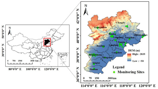
Figure 1.
The distribution of O3 monitoring sites and the topography in the BTH region.
2.2. O3 Monitoring Data
The hourly O3 monitoring data from 1 January 2020 to 31 December 2020 were downloaded from the air pollution monitoring network, which belongs to China National Environmental Monitoring Centre (CNEMC) (https://air.cnemc.cn:18007/ (accessed on 27 July 2022)). Daily maximum 8-h average O3 concentrations were calculated when there are at least 20 maximum 8-h O3 concentration values for one day (see the Supplementary Materials). There were 86 monitoring sites in the BTH region in 2020. Figure 1 shows the topography and distribution of O3 monitoring sites.
2.3. O3 Satellite Data
OMI aboard NASA’s Earth Observing System’s (EOS) Aura satellite collects information by observing backscattered radiation in the earth’s atmosphere and surface. In this study, O3 satellite data were obtained from OMI. Level 0, Level 1B, Level 2, and Level 3 are the four processing levels of OMI data products. The spatial resolution of OMI is 13 × 24 km. It can measure O3 vertical profile, O3 vertical column concentration, aerosols, clouds, and other gas concentrations [52].
The level 2 O3 profile product used in this study has a total of 18 layers in the vertical altitude of the atmosphere from the ground to 0.3 hPa (about 60 km altitude). The ground-level O3 concentration values could be obtained at the lowest layer (from the surface to an altitude of 3 km). The concentration unit for each O3 column is Dobson Unit (DU), which could be converted to µg/m3 using the following formula [53]:
where is the O3 column concentration of each layer (DU), is the pressure difference between the top and bottom layers (hPa), and is the ground-level O3 concentration which is measured in µg/m3.
2.4. BME Analysis
Daily, seasonal, and one-year exposure levels of O3 were simulated based on the BME model. BME analysis was based on MATLAB R2012a and Spatio-temporal Epistemic Knowledge Synthesis Graphical User Interface (SEKS-GUI) software library. The Exponential model, Gaussian model, Cosine Hole model, Sine Hole model, Mexican Hat model, Nugget model, and Spherical model are the seven covariance functions that are available in the BME model. The spatio-temporal variations of O3 residual concentration were characterized by space-time random field (S/TRF). Z represents a random variable of S/TRF, and Z(p) = Z(s,t), where p = (s,t) represents the space/time coordinate, and s and t are the spatial and time position, respectively. The generation of HD and SD in this study were based on O3 residual concentrations, which were calculated as follows:
where VO(s,t) is the O3 monitoring data that meets valid data criteria. According to NAAQS, a daily maximum 8-h average O3 concentration is valid if there are at least 20 maximum 8-h O3 concentration values for one day. Annual maximum 8-h average O3 concentration is considered valid if at least 324 days in a year are available [54]. NO(s,t) is the O3 monitoring data that does not meet valid data criteria and is the distribution of the maximum daily 8-h average O3 concentration at the monitoring site described by a Gaussian probability density function (PDF). OMI(s,t) is the daily O3 satellite data, which is resampled to 1 km × 1 km grid cells by Arcgis 10.3. Since the coordinate points of O3 satellite data and monitoring data in this study were not exactly consistent, the coordinate point of O3 satellite data which was nearest to the monitoring site was selected as the corresponding point of the O3 monitoring data to calculate O3 residual concentrations. Z(s,t) is the estimated result of daily and annual maximum 8-h average O3 concentration at position s and time t, and ZBME(s,t) is O3 residual concentration estimated based on BME at position s and time t.
HD(s,t) = VO(s,t) − OMI(s,t)
SD(s,t) = NO(s,t) − OMI(s,t)
Z(s,t) = OMI(s,t) + ZBME(s,t)
The analysis of the BME model consists of three main stages, which are the prior stage, meta-prior stage, and posterior stage, respectively.
Prior stage The maximum entropy principle is used to obtain the prior probability density function (PDF) which contains the most information about G-KB and is consistent with the actual situation. The G-KB consists of the mean trend function and the covariance function . is obtained by Equation (5).
where = , = . and represent the HD values at their mapping points , = 1,…, and SD values at the mapping points , = +1,…, . is the simulated value at position. is the constant term of normalized constraint. is the vector of a coefficient related to , and is mathematically a vector of the variable G-KB.
Meta-prior stage: The most appropriate expression form is selected for the S-KB, including HD and SD. In this study, O3 residual concentrations were used to generate HD and SD. HD was calculated based on valid O3 monitoring data and satellite data. SD was calculated by using O3 monitoring data which did not meet the criteria and satellite data.
Posterior stage: The prior PDF is transformed into a posterior PDF, which provides the basis for analysis and prediction. The posterior PDF is calculated based on Bayesian conditionalization rules by Equation (6). Then, Equation (7) is used to calculate the simulated mean of each simulated point.
where is the normalization parameter.
2.5. Validation
Leave-one-out cross-validation (LOOCV) and leave-city-out validation were used to evaluate the predictive accuracy of BME. O3 monitoring data from one monitoring site was selected as a testing set, and data of the remaining monitoring sites combined with satellite data were incorporated into BME in the form of residuals as a training set to train the model. Repeating this process until the O3 monitoring data of all the monitoring sites were used once. For leave-city-out validation, O3 monitoring data from one city was selected as a testing set, and data from the remaining cities were selected as a training set to train the model. Repeating this process until the O3 monitoring data of all the cities were used once. The coefficient of determination (R2), the root mean square error (RMSE), the mean absolute error (MAE), the mean prediction error (MPE), and the mean error (ME) between the observed and simulated O3 concentrations were used to evaluate the model performance. R2 can clearly indicate the model performance, and its value should be close to one for accurate estimation [55]. RMSE, MAE, MPE, and ME can reflect the deviation between the observed and simulated O3 concentrations, and their values should be as small as possible.
2.6. Uncertainty Analysis of O3 Concentration Estimations
The mean absolute percentage error (MAPE) between the observed and simulated O3 concentrations was used to quantify the uncertainty of the output results, and the less variation of its value, the more stable the output. It was calculated from Equation (8).
where is the observed O3 concentration, is the simulated O3 concentration, and is the number of samples for each monitoring site.
3. Results
3.1. Descriptive Statistics
In 2020, the hourly, daily, seasonal, and annual variation characteristics of observed O3 concentrations in the BTH region were shown in Figure 2. Hourly observed O3 concentrations were low at night. The levels of O3 gradually increased after 8:00 a.m. (33.8 μg/m3), peaked at 4:00 p.m. (96.7 μg/m3), and then gradually decreased. The variation curve of the observed daily maximum 8-h average O3 concentration presented an inverted “V” shape. The highest daily O3 concentration was recorded on 7 June, with a value of 215.9 μg/m3, while the lowest O3 concentration was 17.2 μg/m3 on 5 January. The observed O3 concentrations were the highest in summer and the lowest in winter, ranging from 49.9 μg/m3 to 140.5 μg/m3. Among 13 cities, the lowest observed annual maximum 8-h average O3 concentration was concentrated in Chengde (82.7 μg/m3), while the highest observed O3 concentration was presented in Hengshui (98.4 μg/m3). The O3 concentration in other cities such as Cangzhou and Handan was also higher, which was 96.9 μg/m3 and 94.5 μg/m3, respectively.
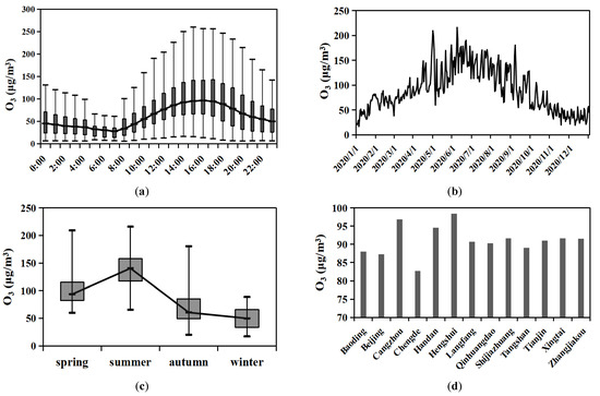
Figure 2.
Variation characteristics of observed O3 concentrations in 2020. (a) hourly O3 concentration, (b) daily maximum 8-h average O3 concentration, (c) seasonal maximum 8-h average O3 concentration, and (d) annual maximum 8-h average O3 concentration in different cities.
3.2. Correlation Analysis between O3 Monitoring and Satellite Data
The correlation between the daily concentrations of O3 monitoring and satellite data is shown in Figure 3. It could be seen that there was a significant positive correlation between the monitoring and satellite data, and Pearson’s correlation coefficient (R) was 0.73. The value for MAE was 30.29 μg/m3, and it reflected the actual situation of the errors between monitoring data and satellite data.
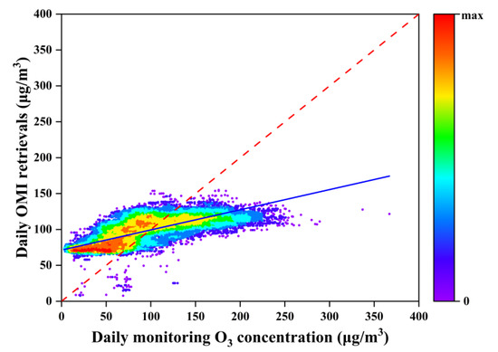
Figure 3.
Correlation of daily O3 concentrations and OMI retrievals. The dashed line is the 1:1 line, while the solid line is the linear regression.
3.3. O3 Daily Exposure
3.3.1. Covariance Model Fitting
Figure 4 shows the covariance function of O3 daily exposure, which provides the spatio-temporal variation information of the O3 residual concentration. The Exponential model for the spatial component and the Gaussian model for the temporal component fitted the best. The fitting effect was better at the position close to the origin, but with the increase in distance and time, the fitting effect gradually decreased. O3 residual concentrations estimated based on the BME model were obtained by using these covariance models.
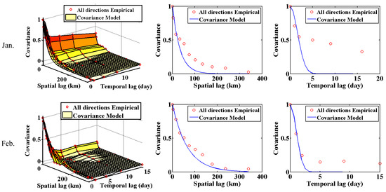
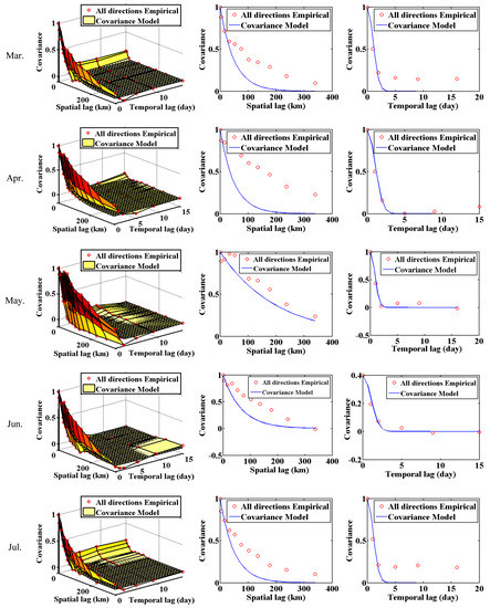
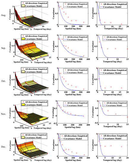
Figure 4.
Observed (red circles) and modeled covariance of the O3 residual concentrations on a daily time scale shown as a function of spatial lag and temporal lag in BME, which showed the spatio-temporal empirical covariance and the fitted model of each month from January to December, respectively.
3.3.2. Validation Results
Figure 5 and Table 1 show the comparison between observed and simulated daily maximum 8-h average O3 concentration in the BTH region based on LOOCV and leave-city-out validation. The values of performance metrics, including R2, RMSE, MAE, MPE, and ME are listed in Table 1. The LOOCV R2 of the simulation results for daily exposure level was 0.81, and the corresponding values for RMSE, MAE, MPE, and ME were 19.58, 14.38, −0.031, and −1.682 μg/m3, respectively. The leave-city-out validation R2 of the simulation results for daily exposure level was 0.83, and the corresponding value for RMSE, MAE, MPE, and ME were 17.12, 12.48, −0.023, and −2.685 μg/m3, respectively.
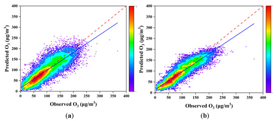
Figure 5.
Scatter plot of observed and simulated daily maximum 8-h average O3 concentration in the BTH region based on LOOCV (a) and leave-city-out validation (b). The dashed line is the 1:1 line, while the solid line is the linear regression.

Table 1.
LOOCV and leave-city-out validation results of BME estimations of daily O3 concentrations.
3.3.3. O3 Daily Exposure Level
Taking the first day of each month as an example, the spatial distributions of the daily maximum 8-h average O3 concentration in the BTH region in 2020 were shown in Figure 6. The lowest simulated daily maximum 8-h average O3 concentration value was on 1 January (21.2 μg/m3) and the highest value was obtained on 7 June (206.3 μg/m3). O3 concentration values in Handan, Hengshui, Cangzhou, and Xingtai were at high levels, while the O3 concentration values in Chengde and Shijiazhuang were low.
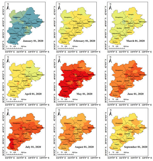
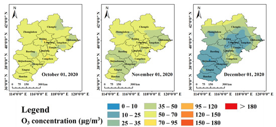
Figure 6.
Spatial distribution of daily maximum 8-h average O3 concentration on the first day of each month.
3.4. O3 One-Year Exposure
3.4.1. Covariance Model Fitting
Figure 7 shows the covariance function of O3 one-year exposure, which provides the spatio-temporal variation information of the O3 residual concentration. The covariance model of BME was composed of a nested model consisting of an Exponential model and a Sine Hole model.
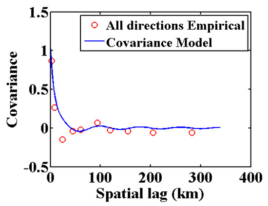
Figure 7.
Observed (red circles) and modeled covariance of the O3 residual concentrations on a one-year time scale shown as a function of spatial lag in BME.
3.4.2. Validation Results
Figure 8 and Table 2 show the comparison between observed and simulated annual maximum 8-h average O3 concentration in the BTH region based on LOOCV and leave-city-out validation. The values of performance metrics are listed in Table 2. The LOOCV R2 of the simulation results for the one-year exposure level was 0.69, and the corresponding values for RMSE, MAE, MPE, and ME were 4.40, 2.60, −0.005, and −0.505 μg/m3, respectively. The leave-city-out validation R2 of the simulation results for the one-year exposure level was 0.61, and the corresponding values for RMSE, MAE, MPE, and ME were 2.54, 2.14, −0.002, and −0.191 μg/m3, respectively. The LOOCV R2 value for the BME model without satellite data was 0.59, and the corresponding values for RMSE, MAE, MPE, and ME were 4.56, 2.83, −0.004, and −0.403 μg/m3, respectively. Therefore, the results simulated by the BME model with satellite data performed better than those without satellite data.
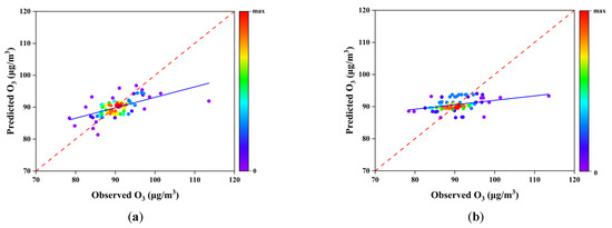
Figure 8.
Scatter plot of observed and simulated annual maximum 8-h average O3 concentration in the BTH region based on LOOCV (a) and leave-city-out validation (b). The dashed line is the 1:1 line, while the solid line is the linear regression.

Table 2.
LOOCV and leave-city-out validation results of BME estimations of annual O3 concentrations.
3.4.3. O3 One-Year Exposure Level
In 2020, the simulated annual maximum 8-h average O3 concentrations for each grid cell varied from 79.5 μg/m3 to 97.5 μg/m3 in the BTH region. Figure 9 shows O3 one-year exposure level based on the BME model. High O3 concentrations were presented in the southeastern BTH region while low O3 concentrations were mainly concentrated in the northwest. The high-value center of O3 concentration was around the southeast of Hebei Province, especially Cangzhou and Hengshui. The O3 concentration was also higher in the northeast of Handan, Xingtai, and the east of Tianjin. The lowest O3 concentration was in Chengde. Other cities including Qinhuangdao, Baoding, and Zhangjiakou also had low O3 concentrations.
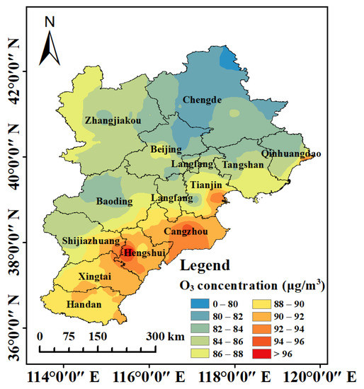
Figure 9.
Spatial distribution of annual maximum 8-h average O3 concentration.
Figure 10 presents the seasonal distributions of O3 concentration in 2020. The highest average O3 concentration value was in summer (134.5 μg/m3), followed by spring (100.9 μg/m3) and autumn (65.3 μg/m3), and the lowest average O3 concentration value was in winter (51.1 μg/m3). Generally, O3 concentrations in the southeastern part of the BTH region were significantly higher than those in the northwestern part of the BTH region. Tianjin, Cangzhou, Hengshui, Xingtai, and Handan had always been the relatively high concentration areas in four seasons. Compared with other cities, the O3 concentration in Chengde was the lowest in all the seasons. For Baoding and Shijiazhuang, the O3 concentration in summer was high and then decreased rapidly in winter. There were significant seasonal and regional differences in O3 concentration in the BTH region. The simulation results of O3 concentration in this study were similar to the published studies [56,57].
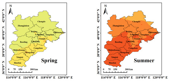
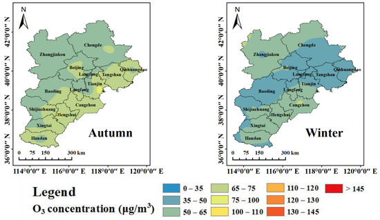
Figure 10.
Spatial distribution of seasonal maximum 8-h average O3 concentration.
3.5. Uncertainty Analysis and Comparisons with NAAQS
Based on Equation (8), the uncertainty analysis of the predicted daily maximum 8-h average O3 concentrations was quantified with values ranging from 15% to 44%. Figure 11 shows the percentages of grids with the daily maximum 8-h average O3 concentrations in the BTH region. As shown in the figure, O3 concentrations in 34.7% of grid-days were more than 100 μg/m3, and 6.8% of these grid-days had serious ozone pollution with O3 concentrations of more than 160 μg/m3 in 2020. In January, February, March, October, November, and December, grid-days with O3 concentrations below 160 µg/m3 and above 100 µg/m3 accounted for less than 7% of the total grid-days, and the highest percentage was in March, with a value of 6.2%. From April to September, daily maximum 8-h average O3 concentrations were higher than 100 μg/m3 on most grid-days. For seasons, the percentage of grids with daily maximum 8-h average O3 concentrations below 100 μg/m3 was 99.2% in winter, while in summer, daily maximum 8-h average O3 concentrations in 87.7% of the grids were higher than 100 μg/m3.
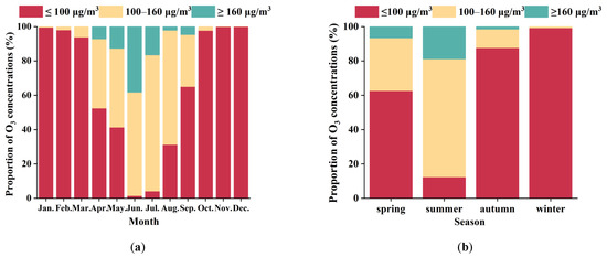
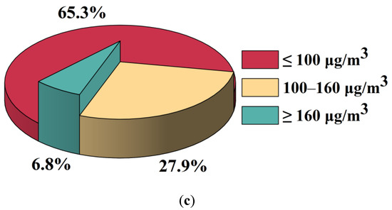
Figure 11.
Percentages of grids with daily maximum 8-h average O3 concentrations below 100 μg/m3, between 100 and 160 μg/m3, and above 160 μg/m3 based on BME in the BTH region. (a) in each month, (b) in each season, and (c) in 2020.
4. Discussion
Liu et al. [58] estimated O3 concentration in China from 2005 to 2017 by a machine learning model, which was based on the eXtreme Gradient Boosting (XGBoost) algorithm, with R2 ranging from 0.61 to 0.78. Qian et al. [59] proposed a hybrid model that integrated multiple variables to estimate ground-level O3 concentration in the continental United States, and the correlation coefficient between the real and simulated values of O3 was 0.76. Lyu et al. [60] predicted daily O3 concentration in the BTH region based on Decision tree (DT) regression, with an R2 value of 0.73. Compared with other research, the BME model used in this study achieved high prediction accuracy in estimating O3 concentration, and LOOCV R2 for the daily and one-year exposure levels were 0.81 and 0.69, respectively. According to the results of estimating O3 concentrations in the BTH region based on an artificial neural network (R2 = 0.8299) and Stepwise regression analysis (R2 = 0.7324) in our research group, the R2 between observed O3 concentration and O3 concentration simulated by the BME model was comparable to the results simulated by the artificial neural network and were higher than the results simulated by the stepwise regression analysis. Huang et al. [61] predicted the annual average O3 concentration in Nanjing based on the LUR model. Fan et al. [62] proposed a spatio-temporal geostatistical kriging interpolation to simulate average monthly O3 concentration based on the composite space/time mean trend (CSTM) model. Compared to these studies, the temporal resolutions of simulated O3 exposure levels in our study were daily, seasonal, and annually, respectively. Zhan et al. [63] predicted the daily maximum 8-h average O3 concentration in mainland China at a resolution of 0.1° × 0.1° based on the random forest model. Zhang et al. [64] used the ordinary kriging (OK) and spatial-temporal kriging (STK) models to simulate the daily maximum 8-h average O3 concentration with a spatial resolution of 2 km × 2 km in the Pearl River Delta (PRD) region, China. However, in this study, we attempted to predict O3 concentration with a high spatial resolution of 1 km × 1 km.
The empirical covariances of O3 exposure reflected the distribution and variation of O3 concentrations in different spatio-temporal coordinates. In this study, the covariance of each month was different, and some months appeared to have poor fitting performance, mainly due to the spatio-temporal dependence of O3 concentrations. Lower covariance values represented greater variability in O3 concentrations and weaker spatio-temporal dependence of O3 concentrations, which increased the difficulty of capturing spatio-temporal features and made the O3 concentration estimations less accurate.
The monitoring data offers the most accurate O3 concentration information, while the satellite data has a wider coverage and can provide more comprehensive information for the estimation of O3 concentrations, and we try to combine the two data to take advantage of their strengths, which improves the accuracy of the simulations. In this study, the BME model with satellite data is effective in improving the accuracy of the O3 exposure level simulations with a 14% increase in the value of LOOCV R2 compared to the BME model without satellite data. We should combine monitoring data with multiple satellite data which has a higher spatio-temporal resolution to simulate O3 exposure levels in the future.
We used LOOCV and leave-city-out validation to evaluate the performance of the BME model in estimating daily and annual maximum 8-h average O3 concentrations. The results showed that for daily exposure levels, the LOOCV R2 was 0.81, while the corresponding value based on leave-city-out validation was 0.83, which was slightly higher than the value based on LOOCV. For the one-year exposure level, the LOOCV R2 was higher than the corresponding value based on the leave-city-out validation. The LOOCV was probably suitable for estimating predictions for representative points near monitors, but leave-city-out validation was more useful to evaluate the performance of the model when predicting unsampled sites which were far from monitors. In this study, the number of monitoring sites that met the valid data criteria varied on each day, resulting in different sizes of training sets for each day to train the model based on LOOCV and leave-city-out validation, respectively, which might lead to a slightly higher value for R2 based on leave-city-out validation than that based on LOOCV.
In terms of spatial distribution, O3 concentrations in the southeastern part of the BTH region were high throughout the year, while O3 concentrations were low in the northwestern part of the BTH region. The high value was mainly located in the southeast of the Hebei Province, especially in Cangzhou, Hengshui, Handan, Xingtai, and Tianjin. The pillar industries in these cities are mainly heavy industries, which produced large amounts of precursors such as VOCs and NOx in the atmosphere that may ultimately affect O3 concentration [65,66]. Compared with 2019, the number of civil vehicles owned in Beijing, Tianjin, and Hebei in 2020 increased by 3.2%, 6.9%, and 5.8%, respectively [67,68,69]. The photochemical reaction of NOx emitted by vehicles would also increase the concentration of O3. The area with the lowest O3 concentration was located in Chengde. Chengde prioritized the development of tourism as the first leading industry and gradually adjusted the industrial structure of heavy and chemical industries, so the pollutant emissions gradually decreased, which might explain the reason why O3 concentration was low in most areas of Chengde.
The diurnal variation of O3 concentration was closely related to the photochemical reaction. The photochemical reaction was weak at night, so O3 concentration gradually decreased, reaching the lowest value at 8:00 a.m. The increase in solar radiation and temperature intensified the photochemical reaction, and O3 concentration reached the highest value at 4:00 p.m., then gradually decreased. The seasonal variation of O3 concentration was significantly associated with meteorological factors such as wind speed, temperature, relative humidity, as well as solar radiation. Several studies showed that O3 concentration was positively associated with wind speed and temperature and was negatively associated with relative humidity [70,71,72]. In spring, a dry climate, less precipitation, and strong solar radiation were conducive to O3 generation. Meanwhile, wind speed reflected the turbulent movement of the boundary layer. Increased wind speed accelerates atmospheric mixing and promotes the exchange between the air with higher O3 concentration in the upper boundary layer and the air with lower O3 concentration in the lower layer. As a result, the higher O3 concentration air might intrude from the upper boundary layer to the lower layer, thus increasing the ground-level O3 concentration [73]. In summer, intense solar radiation and sustained high temperature led to increased photochemical reactions produced by NOx and VOCs in the atmosphere, and relative humidity was low, which exacerbated O3 pollution [74,75]. The atmosphere was relatively stable in autumn and winter, which was not conducive to the dilution, diffusion, and local transport of pollutants, thus inhibiting O3 generation [76]. At the same time, the solar radiation was weak, and the temperature was low, which was not conducive to photochemical reactions, so O3 concentration was low.
There are a few limitations in our study. Firstly, the low spatial resolution of the OMI O3 profile may affect the accuracy of the model prediction. With the gradual development of satellites, satellite data with more details and higher resolutions could be used to get more accurate results. Secondly, we used one model to estimate the O3 exposure level. In future studies, multiple models could be combined and compared to estimate pollutant exposure levels with higher resolution and accuracy.
5. Conclusions
The daily, seasonal, and annual maximum 8-h average O3 concentrations in the BTH region at a 1 km × 1 km resolution were estimated based on the BME model. The BME model with satellite data can significantly improve the simulation of O3 exposure levels, with LOOCV R2 being 0.10 higher than the corresponding value simulated by the BME model without satellite data, and the values for RMSE, MAE, MPE, and ME simulated by BME model were 0.16, 0.23, 0.001, and 0.102 μg/m3 lower, respectively than the values simulated by BME model without satellite data. The results indicate that the BME model with satellite data performs better than the model without satellite data in simulating O3 concentrations. The spatio-temporal maps of O3 concentrations generated by BME could be used to characterize the variability of O3 concentrations. The BME is capable of simulating O3 exposure levels with high spatio-temporal resolution. The simulated O3 concentrations provide valuable information, which has the potential to improve health risk assessment, provide assistance for future epidemiological studies, and inform reference for the choice of appropriate modeling methods in future related studies.
Supplementary Materials
The following are available online at https://www.mdpi.com/article/10.3390/atmos13101568/s1, Daily maximum 8-h average O3 concentrations in the BTH region, China in 2020.
Author Contributions
Conceptualization, L.C.; Data curation, S.X., C.C. and Z.Q.; Methodology, S.X., C.C. and L.C.; Software, S.X. and M.S.; Supervision, Z.M.; Visualization, H.Z., S.G. and Y.S.; Writing—original draft, S.X.; Writing—review & editing, C.C., M.S., Y.L. and L.C. All authors have read and agreed to the published version of the manuscript.
Funding
This study was funded by the National Key Research and Development Program (Grants No. 2016YFC0201700).
Institutional Review Board Statement
Not applicable.
Informed Consent Statement
Not applicable.
Data Availability Statement
China National Environmental Monitoring Centre. China Air Quality Data. Available online: https://air.cnemc.cn:18007/ (accessed on 27 July 2022); NASA. Satellite Data. Available online: https://disc.gsfc.nasa.gov/datasets/OMO3PR_003/summary (accessed on 27 July 2022).
Conflicts of Interest
The authors declare no conflict of interest.
References
- Qi, B.; Niu, Y.Y.; Du, R.G.; Yu, Z.F.; Ying, F.; Xu, H.H.; Hong, S.M.; Yang, H.Q. Characteristics of surface ozone concentration in urban site of Hangzhou. China Environ. Sci. 2017, 37, 443–451. (In Chinese) [Google Scholar]
- Chen, B.; Yang, X.B.; Xu, J.J. Spatio-temporal variation and influencing factors of ozone pollution in Beijing. Atmosphere 2022, 13, 359. [Google Scholar] [CrossRef]
- Rich, D.Q.; Balmes, J.R.; Frampton, M.W.; Zareba, W.; Stark, P.; Arjomandi, M.; Hazucha, M.J.; Costantini, M.G.; Ganz, P.; Hollenbeck-Pringle, D.; et al. Cardiovascular function and ozone exposure: The multicenter ozone study in older subjects (moses). Environ. Int. 2018, 119, 193–202. [Google Scholar] [CrossRef] [PubMed]
- Xia, Y.J.; Niu, Y.; Cai, J.; Lin, Z.J.; Liu, C.; Li, H.C.; Chen, C.; Song, W.M.; Zhao, Z.H.; Chen, R.J.; et al. Effects of personal short-term exposure to ambient ozone on blood pressure and vascular endothelial function: A mechanistic study based on DNA methylation and metabolomics. Environ. Sci. Technol. 2018, 52, 12774–12782. [Google Scholar] [CrossRef] [PubMed]
- Lin, C.Y.; Ma, Y.Q.; Liu, R.Y.; Shao, Y.C.; Ma, Z.W.; Zhou, L.; Jing, Y.S.; Bell, M.L.; Chen, K. Associations between short-term ambient ozone exposure and cause-specific mortality in rural and urban areas of Jiangsu, China. Environ. Res. 2022, 211, 113098. [Google Scholar] [CrossRef] [PubMed]
- Glasgow, G.; Smith, A. Uncertainty in the estimated risk of lung function decrements owing to ozone exposure. J. Expo. Sci. Environ. Epidemiol. 2017, 27, 535–538. [Google Scholar] [CrossRef]
- Huang, J.; Li, G.X.; Xu, G.Z.; Qian, X.J.; Zhao, Y.; Pan, X.C.; Huang, J.; Cen, Z.D.; Liu, Q.C.; He, T.F.; et al. The burden of ozone pollution on years of life lost from chronic obstructive pulmonary disease in a city of Yangtze River Delta, China. Environ. Pollut. 2018, 242, 1266–1273. [Google Scholar] [CrossRef]
- Zhou, P.E.; Qian, Z.M.; McMillin, S.E.; Vaughn, M.G.; Xie, Z.Y.; Xu, Y.J.; Lin, L.Z.; Hu, L.W.; Yang, B.Y.; Zeng, X.W.; et al. Relationships between long-term ozone exposure and allergic rhinitis and bronchitic symptoms in Chinese children. Toxics 2021, 9, 221. [Google Scholar] [CrossRef]
- Zu, K.; Liu, X.B.; Shi, L.H.; Tao, G.; Loftus, C.T.; Lange, S.; Goodman, J.E. Concentration-response of short-term ozone exposure and hospital admissions for asthma in Texas. Environ. Int. 2017, 104, 139–145. [Google Scholar] [CrossRef]
- Cleary, E.G.; Cifuentes, M.; Grinstein, G.; Brugge, D.; Shea, T.B. Association of low-level ozone with cognitive decline in older adults. J. Alzheimers Dis. 2018, 61, 67–78. [Google Scholar] [CrossRef]
- Gao, Q.; Zang, E.M.; Bi, J.; Dubrow, R.; Lowe, S.R.; Chen, H.S.; Zeng, Y.; Shi, L.H.; Chen, K. Long-term ozone exposure and cognitive impairment among Chinese older adults: A cohort study. Environ. Int. 2022, 160, 107072. [Google Scholar] [CrossRef] [PubMed]
- Jung, C.R.; Lin, Y.T.; Hwang, B.F. Ozone, particulate matter, and newly diagnosed Alzheimer’s disease: A population-based cohort study in Taiwan. J. Alzheimers Dis. 2015, 44, 573–584. [Google Scholar] [CrossRef] [PubMed]
- Liu, H.; Liu, S.; Xue, B.R.; Lv, Z.F.; Meng, Z.H.; Yang, X.F.; Xue, T.; Yu, Q.; He, K.B. Ground-level ozone pollution and its health impacts in China. Atmos. Environ. 2018, 173, 223–230. [Google Scholar] [CrossRef]
- Seltzer, K.M.; Shindell, D.T.; Malley, C.S. Measurement-based assessment of health burdens from long-term ozone exposure in the United States, Europe, and China. Environ. Res. Lett. 2018, 13, 104018. [Google Scholar] [CrossRef]
- Feng, Z.Z.; De Marco, A.; Anav, A.; Gualtieri, M.; Sicard, P.; Tian, H.Q.; Fornasier, F.; Tao, F.L.; Guo, A.H.; Paoletti, E. Economic losses due to ozone impacts on human health, forest productivity and crop yield across China. Environ. Int. 2019, 131, 104966. [Google Scholar] [CrossRef] [PubMed]
- Li, P.; Feng, Z.Z.; Catalayud, V.; Yuan, X.Y.; Xu, Y.S.; Paoletti, E. A meta-analysis on growth, physiological, and biochemical responses of woody species to ground-level ozone highlights the role of plant functional types. Plant Cell Environ. 2017, 40, 2369–2380. [Google Scholar] [CrossRef] [PubMed]
- Ministry of Ecology and Environment of the people’s Republic of China. Bulletin of the State of the Environment in China for Year 2018. Available online: https://www.mee.gov.cn/hjzl/sthjzk/zghjzkgb/201905/P020190619587632630618.pdf (accessed on 27 July 2022).
- Ministry of Ecology and Environment of the People’s Republic of China. Bulletin of the State of the Environment in China for Year 2020. Available online: https://www.mee.gov.cn/hjzl/sthjzk/zghjzkgb/202105/P020210526572756184785.pdf (accessed on 27 July 2022).
- Liang, S.; Li, X.; Teng, Y.; Fu, H.; Chen, L.; Mao, J.; Zhang, H.; Gao, S.; Sun, Y.; Ma, Z.; et al. Estimation of health and economic benefits based on ozone exposure level with high spatial-temporal resolution by fusing satellite and station observations. Environ. Pollut. 2019, 255, 113267. [Google Scholar] [CrossRef]
- Chen, L.; Gao, S.; Zhang, H.; Sun, Y.L.; Ma, Z.X.; Vedal, S.; Mao, J.; Bai, Z.P. Spatiotemporal modeling of PM2.5 concentrations at the national scale combining land use regression and Bayesian maximum entropy in China. Environ. Int. 2018, 116, 300–307. [Google Scholar] [CrossRef]
- Streets, D.G.; Bond, T.C.; Carmichael, G.R.; Fernandes, S.D.; Fu, Q.; He, D.; Klimont, Z.; Nelson, S.M.; Tsai, N.Y.; Wang, M.Q.; et al. An inventory of gaseous and primary aerosol emissions in Asia in the year 2000. J. Geophys. Res. Atmos. 2003, 108, 8809. [Google Scholar] [CrossRef]
- Zhang, L.; Jacob, D.J.; Boersma, K.F.; Jaffe, D.A.; Olson, J.R.; Bowman, K.W.; Worden, J.R.; Thompson, A.M.; Avery, M.A.; Cohen, R.C.; et al. Transpacific transport of ozone pollution and the effect of recent Asian emission increases on air quality in North America: An integrated analysis using satellite, aircraft, ozonesonde, and surface observations. Atmos. Chem. Phys. 2008, 8, 6117–6136. [Google Scholar] [CrossRef]
- Wang, J.W.; Cohan, D.S.; Xu, H. Spatiotemporal ozone pollution LUR models: Suitable statistical algorithms and time scales for a megacity scale. Atmos. Environ. 2020, 237, 117671. [Google Scholar] [CrossRef]
- Liu, Z.Y.; Guan, Q.Y.; Lin, J.K.; Yang, L.Q.; Luo, H.P.; Wang, N. A new buffer selection strategy for Land use regression model of PM2.5 in Xi’an, China. Environ. Sci. Pollut. Res. 2021, 28, 21245–21255. [Google Scholar] [CrossRef] [PubMed]
- Meng, X.; Chen, L.; Cai, J.; Zou, B.; Wu, C.F.; Fu, Q.Y.; Zhang, Y.; Liu, Y.; Kan, H.D. A land use regression model for estimating the NO2 concentration in Shanghai, China. Environ. Res. 2015, 137, 308–315. [Google Scholar] [CrossRef] [PubMed]
- Muttoo, S.; Ramsay, L.; Brunekreef, B.; Beelen, R.; Meliefste, K.; Naidoo, R.N. Land use regression modeling estimating nitrogen oxides exposure in industrial South Durban, South Africa. Sci. Total Environ. 2018, 610, 1439–1447. [Google Scholar] [CrossRef] [PubMed]
- Rahman, M.M.; Yeganeh, B.; Clifford, S.; Knibbs, L.D.; Morawska, L. Development of a Land use regression model for daily NO2 and NOx concentrations in the Brisbane metropolitan area, Australia. Environ. Model. Softw. 2017, 95, 168–179. [Google Scholar] [CrossRef]
- Meyer, H.; Reudenbach, C.; Hengl, T.; Katurji, M.; Nauss, T. Improving performance of spatio-temporal machine learning models using forward feature selection and target-oriented validation. Environ. Model. Softw. 2018, 101, 1–9. [Google Scholar] [CrossRef]
- Ren, X.; Mi, Z.; Georgopoulos, P.G. Comparison of machine learning and land use regression for fine scale spatiotemporal estimation of ambient air pollution: Modeling ozone concentrations across the contiguous united states. Environ. Int. 2020, 142, 105827. [Google Scholar] [CrossRef]
- Konakoglu, B.; Akar, A. Prediction of geoid undulation using approaches based on GMDH, M5 model tree, MARS, GPR, and IDP. Acta Geod. Geophys. 2022, 57, 293–315. [Google Scholar] [CrossRef]
- Keshtegar, B.; Mert, C.; Kisi, O. Comparison of four heuristic regression techniques in solar radiation modeling: Kriging method vs RSM, MARS and M5 model tree. Renew. Sustain. Energy Rev. 2018, 81, 330–341. [Google Scholar] [CrossRef]
- Gholampour, A.; Mansouri, I.; Kisi, O.; Ozbakkaloglu, T. Evaluation of mechanical properties of concretes containing coarse recycled concrete aggregates using multivariate adaptive regression splines (MARS), M5 model tree (M5Tree), and least squares support vector regression (LSSVR) models. Neural Comput. Appl. 2020, 32, 295–308. [Google Scholar] [CrossRef]
- Deo, R.C.; Kisi, O.; Singh, V.P. Drought forecasting in eastern Australia using multivariate adaptive regression spline, least square support vector machine and M5Tree model. Atmos. Res. 2017, 184, 149–175. [Google Scholar] [CrossRef]
- Kisi, O.; Khosravinia, P.; Nikpour, M.R.; Sanikhani, H. Hydrodynamics of river-channel confluence: Toward modeling separation zone using GEP, MARS, M5 Tree and DENFIS techniques. Stoch. Environ. Res. Risk Assess. 2019, 33, 1089–1107. [Google Scholar] [CrossRef]
- Qin, Q.Q.; Wang, H.Y.; Lei, X.D.; Li, X.; Xie, Y.L.; Zheng, Y.L. Spatial variability in the amount of forest litter at the local scale in northeastern China: Kriging and cokriging approaches to interpolation. Ecol. Evol. 2020, 10, 778–790. [Google Scholar] [CrossRef] [PubMed]
- Zou, B.; Luo, Y.Q.; Wan, N.; Zheng, Z.; Sternberg, T.; Liao, Y.L. Performance comparison of LUR and OK in PM2.5 concentration mapping: A multidimensional perspective. Sci. Rep. 2015, 5, 8698. [Google Scholar] [CrossRef]
- Zhang, Q.Q.; Zhang, X.Y. Ozone spatial-temporal distribution and trend over China since 2013: Insight from satellite and surface observation. Environ. Sci. 2019, 40, 1132–1142. [Google Scholar]
- Cleland, S.E.; West, J.J.; Jia, Y.Q.; Reid, S.; Raffuse, S.; O’Neill, S.; Serre, M.L. Estimating wildfire smoke concentrations during the October 2017 California fires through BME space/time data fusion of observed, modeled, and satellite-derived PM2.5. Environ. Sci. Technol. 2020, 54, 13439–13447. [Google Scholar] [CrossRef]
- Hayunga, D.K.; Kolovos, A. Geostatistical space-time mapping of house prices using Bayesian maximum entropy. Int. J. Geogr. Inf. Sci. 2016, 30, 2339–2354. [Google Scholar] [CrossRef]
- Xu, Y.D.; Serre, M.L.; Reyes, J.; Vizuete, W. Bayesian maximum entropy integration of ozone observations and model predictions: A national application. Environ. Sci. Technol. 2016, 50, 4393–4400. [Google Scholar] [CrossRef]
- Ellison, A.M. Bayesian inference in ecology. Ecol. Lett. 2004, 7, 509–520. [Google Scholar] [CrossRef]
- DeLang, M.N.; Becker, J.S.; Chang, K.L.; Serre, M.L.; Cooper, O.R.; Schultz, M.G.; Schroder, S.; Lu, X.; Zhang, L.; Deushi, M.; et al. Mapping yearly fine resolution global surface ozone through the Bayesian maximum entropy data fusion of observations and model output for 1990-2017. Environ. Sci. Technol. 2021, 55, 4389–4398. [Google Scholar] [CrossRef]
- McCarthy, M.A.; Masters, P. Profiting from prior information in Bayesian analyses of ecological data. J. Appl. Ecol. 2005, 42, 1012–1019. [Google Scholar] [CrossRef]
- Yu, H.L.; Chen, J.C.; Christakos, G.; Jerrett, M. BME estimation of residential exposure to ambient PM10 and ozone at multiple time scales. Environ. Health Perspect. 2009, 117, 537–544. [Google Scholar] [CrossRef] [PubMed][Green Version]
- Jiang, Q.T.; Christakos, G. Space-time mapping of ground-level PM2.5 and NO2 concentrations in heavily polluted northern China during winter using the Bayesian maximum entropy technique with satellite data. Air Qual. Atmos. Health 2018, 11, 23–33. [Google Scholar] [CrossRef]
- He, J.Y.; Kolovos, A. Bayesian maximum entropy approach and its applications: A review. Stoch. Environ. Res. Risk Assess. 2018, 32, 859–877. [Google Scholar] [CrossRef]
- Christakos, G.; Serre, M.L. BME analysis of spatiotemporal particulate matter distributions in North Carolina. Atmos. Environ. 2000, 34, 3393–3406. [Google Scholar] [CrossRef]
- Bogaert, P.; Christakos, G.; Jerrett, M.; Yu, H.L. Spatiotemporal modelling of ozone distribution in the state of California. Atmos. Environ. 2009, 43, 2471–2480. [Google Scholar] [CrossRef]
- De Nazelle, A.; Arunachalam, S.; Serre, M.L. Bayesian maximum entropy integration of ozone observations and model predictions: An application for attainment demonstration in North Carolina. Environ. Sci. Technol. 2010, 44, 5707–5713. [Google Scholar] [CrossRef]
- Chen, L.; Liang, S.; Li, X.L.; Mao, J.; Gao, S.; Zhang, H.; Sun, Y.L.; Vedal, S.; Bai, Z.P.; Ma, Z.X.; et al. A hybrid approach to estimating long-term and short-term exposure levels of ozone at the national scale in China using Land use regression and Bayesian maximum entropy. Sci. Total Environ. 2021, 752, 141780. [Google Scholar] [CrossRef]
- Mei, Y.Y.; Li, J.Y.; Xiang, D.P.; Zhang, J.X. When a generalized linear model meets Bayesian maximum entropy: A novel spatiotemporal ground-level ozone concentration retrieval method. Remote Sens. 2021, 13, 4324. [Google Scholar] [CrossRef]
- NASA. Ozone Monitoring Instrument (OMI) Data User’s Guide. 2012. Available online: https://docserver.gesdisc.eosdis.nasa.gov//repository/Mission/OMI/3.3_ScienceDataProductDocumentation/3.3.2_ProductRequirements_Designs/README.OMI_DUG.pdf (accessed on 27 July 2022).
- Liu, X.Z.; Lou, S.R.; Chen, Y.H.; Liu, Q.; Wang, J.; Shan, Y.Y.; Huang, S.J.; Du, H.J. Spatiotemporal distribution of ground-level ozone in mid-east China based on OMI observations. Acta Sci. Circumstantiae 2016, 36, 2811–2818. (In Chinese) [Google Scholar]
- GB 3095-2012; Ambient Air Quality Standards. Ministry of Ecology and Environment of the People’s Republic of China: Beijing, China, 2012. Available online: https://www.mee.gov.cn/ywgz/fgbz/bz/bzwb/dqhjbh/dqhjzlbz/201203/W020120410330232398521.pdf (accessed on 27 July 2022).
- Chicco, D.; Warrens, M.J.; Jurman, G. The coefficient of determination R-squared is more informative than SMAPE, MAE, MAPE, MSE and RMSE in regression analysis evaluation. PeerJ Comput. Sci. 2021, 7, e623. [Google Scholar] [CrossRef] [PubMed]
- Hu, L.M.; Li, Y.X.; Shi, N.F.; Su, Y. Spatio-temporal change characteristics of ozone concentration in Beijing-Tianjin-Hebei region. Environ. Sci. Technol. 2019, 42, 1–7+39. (In Chinese) [Google Scholar]
- Wang, Z.B.; Li, J.X.; Liang, L.W. Spatio-temporal evolution of ozone pollution and its influencing factors in the Beijing-Tianjin-Hebei urban agglomeration. Environ. Pollut. 2020, 256, 113419. [Google Scholar] [CrossRef] [PubMed]
- Liu, R.; Ma, Z.; Liu, Y.; Shao, Y.; Zhao, W.; Bi, J. Spatiotemporal distributions of surface ozone levels in China from 2005 to 2017: A machine learning approach. Environ. Int. 2020, 142, 105823. [Google Scholar] [CrossRef] [PubMed]
- Qian, D.; Sebastian, R.; Petros, K.; Joel, S. A hybrid model for spatially and temporally resolved ozone exposures in the continental united states. J. Air Waste Manag. Assoc. 2017, 67, 39–52. [Google Scholar]
- Lyu, Y.; Ju, Q.R.; Lv, F.M.; Feng, J.L.; Pang, X.B.; Li, X. Spatiotemporal variations of air pollutants and ozone prediction using machine learning algorithms in the Beijing-Tianjin-Hebei region from 2014 to 2021. Environ. Pollut. 2022, 306, 119420. [Google Scholar] [CrossRef]
- Huang, L.; Zhang, C.; Bi, J. Development of land use regression models for PM2.5, SO2, NO2 and O3 in Nanjing, China. Environ. Res. 2017, 158, 542–552. [Google Scholar] [CrossRef]
- Fan, Z.R.; Huang, B.H.; Peng, C.; Lin, J.Y.; Liao, Y.L. Simulation of average monthly ozone exposure concentrations in China: A temporal and spatial estimation method. Environ. Res. 2021, 199, 111271. [Google Scholar] [CrossRef]
- Zhan, Y.; Luo, Y.Z.; Deng, X.F.; Grieneisen, M.L.; Zhang, M.H.; Di, B.F. Spatiotemporal prediction of daily ambient ozone levels across China using random forest for human exposure assessment. Environ. Pollut. 2018, 233, 464–473. [Google Scholar] [CrossRef]
- Zhang, A.; Lin, J.H.; Chen, W.H.; Lin, M.S.; Lei, C.C. Spatial-temporal distribution variation of ground-level ozone in China’s Pearl River Delta metropolitan region. Int. J. Environ. Res. Public Health 2021, 18, 872. [Google Scholar] [CrossRef]
- Zhu, L.; Liu, M.X.; Song, J.Y. Spatiotemporal variations and influent factors of tropospheric ozone concentration over China based on OMI data. Atmosphere 2022, 13, 253. [Google Scholar] [CrossRef]
- Meng, X.; Wang, W.D.; Shi, S.; Zhu, S.Q.; Wang, P.; Chen, R.J.; Xiao, Q.Y.; Tao, X.; Geng, G.N.; Zhang, Q.; et al. Evaluating the spatiotemporal ozone characteristics with high-resolution predictions in mainland China, 2013–2019. Environ. Pollut. 2022, 299, 118865. [Google Scholar] [CrossRef] [PubMed]
- Beijing Bureau of Statistics of China. Beijing Statistical Year Book 2021; China Statistics Press: Beijing, China, 2021; Available online: http://nj.tjj.beijing.gov.cn/nj/main/2021-tjnj/zk/indexch.htm (accessed on 27 July 2022).
- Hebei Bureau of Statistics of China. Hebei Statistical Year Book 2021; China Statistics Press: Hebei, China, 2021; Available online: http://tjj.Hebei.Gov.Cn/hetj/tjnj/2021/zk/indexch.htm (accessed on 27 July 2022).
- Tianjin Bureau of Statistics of China. Tianjin Statistical Year Book 2021; China Statistics Press: Tianjin, China, 2021; Available online: http://stats.tj.gov.cn/nianjian/2021nj/zk/indexch.htm (accessed on 27 July 2022).
- Dueñas, C.; Fernández, M.C.; Cañete, S.; Carretero, J.; Liger, E. Assessment of ozone variations and meteorological effects in an urban area in the mediterranean coast. Sci. Total Environ. 2002, 299, 97–113. [Google Scholar] [CrossRef]
- Shan, W.; Yin, Y.; Zhang, J.; Ding, Y. Observational study of surface ozone at an urban site in east China. Atmos. Res. 2008, 89, 252–261. [Google Scholar] [CrossRef]
- Toh, Y.Y.; Lim, S.F.; Glasow, R.V. The influence of meteorological factors and biomass burning on surface ozone concentrations at Tanah rata, Malaysia. Atmos. Environ. 2013, 70, 435–446. [Google Scholar] [CrossRef]
- Tu, J.; Xia, Z.-G.; Wang, H.; Li, W. Temporal variations in surface ozone and its precursors and meteorological effects at an urban site in China. Atmos. Res. 2007, 85, 310–337. [Google Scholar] [CrossRef]
- Allu, S.K.; Srinivasan, S.; Maddala, R.K.; Reddy, A.; Anupoju, G.R. Seasonal ground level ozone prediction using multiple linear regression (MLR) model. Modeling Earth Syst. Environ. 2020, 6, 1981–1989. [Google Scholar] [CrossRef]
- Gao, C.; Xiu, A.J.; Zhang, X.L.; Chen, W.W.; Liu, Y.; Zhao, H.M.; Zhang, S.C. Spatiotemporal characteristics of ozone pollution and policy implications in northeast China. Atmos. Pollut. Res. 2020, 11, 357–369. [Google Scholar] [CrossRef]
- Yu, R.L.; Lin, Y.L.; Zou, J.H.; Dan, Y.B.; Cheng, C. Review on atmospheric ozone pollution in China: Formation, spatiotemporal distribution, precursors and affecting factors. Atmosphere 2021, 12, 1675. [Google Scholar] [CrossRef]
Publisher’s Note: MDPI stays neutral with regard to jurisdictional claims in published maps and institutional affiliations. |
© 2022 by the authors. Licensee MDPI, Basel, Switzerland. This article is an open access article distributed under the terms and conditions of the Creative Commons Attribution (CC BY) license (https://creativecommons.org/licenses/by/4.0/).