Abstract
The objective of this work was to modify the HEC-HMS flood prediction for the karstic watershed of the Lijiang River, South China, through the quantitative inclusion into the model of the available reservoir capacity of karst (ARCK) as a case study. Due to the complexities caused by hidden drainage networks in karst hydrology, as a new approach, soil moisture accounting loss was used to reflect the ARCK in flood forecasting. The soil moisture loss was analyzed against daily rainfall runoff data across 1.5 years by using an artificial neural network via phyton programming. Through the correlations found among the amounts of soil moisture and river flow fluctuations in response to precipitation and its intervals, coefficients were introduced to the model for output modifications. ARCK analysis revealed that while heavy rainfalls with longer intervals (i.e., 174 mm/2d after 112 days of the dry season) may not cause considerable changes in the river flow magnitude (0.1–0.64 higher owing to high ARCK), relatively small rainfalls with higher frequency (i.e., 83 mm/4d during the wet season) can cause drastic raise of river flow (10–20 times greater at different stations) due to lower ARCK. Soil moisture accounting loss coefficients did enhance the model’s simulated hydrographs accuracy (NSE) up to 16% on average as compared to the initial forecasting via real data. However, the modifications were valid for flood events within a few years from the soil moisture observation period. Our result suggested that the inclusion of ARCK in modeling through soil moisture accounting loss can lead to increased prediction accuracy through consistent monitoring.
1. Introduction
The majority (94%) of the current 1.45 billion population of China are living in the eastern part of the Hu line, crossing from northeast to southwest which is around 43% of the country. This is historically mainly due to the climate and resources [1]. Among the three largest rivers of China (Yangtze, Yellow, and Pearl Rivers), the last, with its tributaries, is meandering through the subtropical (and some karstic) regions of the country owing to high annual precipitation. Therefore, the main natural disaster in these areas is annual flooding. Controlling and minimizing damages from flooding [2] requires the study of the drivers and influencing factors. In karstic areas, parent rocks are made of carbonate materials, including limestone, dolostone, or gypsum. Karst in humid areas, such as southeast Asia [3], is in constant contact with water, when combined with carbon dioxide produces carbonic acid. The gradual dissolution of these structures occurs due to the movement of weakly acidic water through the pores that leave behind cracks [4]. This will impact the water’s movement patterns and flood formation processes. While due to the infiltration rate limitations, water flux in soil pores can only continue at a relatively slow rate underground; however, karstic fissures and shafts can directly channel the flow within a shorter period and in higher magnitudes. Moreover, water may be retained in voids or join aquifers which slows its traveling time and lowers peak flooding. Hence, karst hydrology is among the most difficult hydrological topics due to its unique features such as open basins (not closed, as hidden drainage networks can have inflow to or outflow from the watershed). Inaccuracies and uncertainties of flood prediction in karstic basins, even via applying models, is an identified problem [5].
On the other hand, due to the complexity of flood routing and the involvement of a wide range of environmental criteria, computer models have been developed to include numerous influencing factors and carry out big data processing and analysis. One of these models, which has been widely used in this field, is HEC-HMS, or hydrologic engineering Canter’s–hydrologic modelling system [6,7,8,9]. The model initially used unit hydrograph (Snyder or SCS) and later Muskingum for flood routing [10,11,12]. However, since most of these models involve empirical formulas, which are environment-dependent, the simulation accuracy in different environments varies and, for that reason, usually requires modification and calibration [13,14]. This is more transpicuous when it comes to a unique environment such as karst. Karstic sinkholes were analyzed in detailed with hydrograph modeling via a new two-piece model developed for recession limb [15,16]. Perhaps one of the most well-known modified models for karst condition is K-XAJ, introduced by Zhou et al. [17]. Although soil moisture accounting has been more widely used in soil modeling, hydrological soil moisture is a less studied subject [18]. Ghazanfari et al. did apply the soil moist accounting effect on evaporation and transpiration over- and underestimation using satellite data on the Indus River watershed [19]. Soil moisture accounting loss has been applied in a number of works to modify different models and formulas. Wang discussed the relationship between the soil wetting capacity and precipitation and its impact on hydrological parameters such as soil conservation service–curve number (SCS-CN) calculations and proposed a new function to describe the ratio between these two parameters for a better determination of the surface flow [20].
Few works on flood analysis in the Lijiang watershed have emphasized the importance of karst on flood formation in this catchment [21,22]. Huang described the contribution of the groundwater as runoff into the total water budget of Guilin karst as significant [23]. Rad et al. indicated that the main reason behind the flood’s different behavior up- and midstream of Lijiang is its unique karst condition [24]. Cao et al. studied the models’ uncertainties and their dependency on the environment in the Lijiang watershed [25]. Xu et al. characterized the Lijiang flood as having uneven annual distribution upstream with an increasing trend since 1954 [26]. A promising study on enhancing HEC-HMS prediction for karst areas of Baise, Guangxi, was recently performed with a 22% accuracy enhancement [10]. However, an efficient modification of the applied models has not been presented yet.
Karst drainage volume and required discharge time are not predictable because it depends on multiple variables, some unmeasurable. The environmental influencing factors are such as geology, morphology, sinkhole location and size, unknown buried flows, inflow rates, runoff, in- and outflow currents, caves and networks, rainfall intervals, and karst stormwater stagnation capacity [27], just to mention few. These make it difficult to quantitively calculate the karst contribution rate in flood. Therefore, we attempted to predict the value of the available reservoir capacity of karst (ARCK) from the measurable variables such as rainfall-runoff, intervals, and soil moisture using an artificial neural network to form a function that incorporates ARCK into the equations. The main aim of this work was to include the soil moisture accounting loss, as representative of karst reservoir capacity fluctuation, in the HEC-HMS model accurate predictions of flood hydrographs of our primary flood simulations in this karst area were found to be strongly dependent to the initial abstraction and condition. This research is important as it helps to have more efficient river management for decision-makers. Especially since, for a lot of people living in these scenic karst areas, Lijiang is a main financial resource [28,29].
2. Materials and Methods
2.1. Study Area
Karstic areas of southeast China cover 1760 km2, which spread over a few provinces, including Guangxi. Guilin city (109°36′–111°29′ E, 24°15′–26°23′ N) is in the northeast part of this province with a total area of 27,800 km2 (including the suburbs), and 5200 km2 of it is covered by karst. More than 250 km2 of it is listed on UNESCO’s world heritage committee (WHC) since 2014 [30]. Based on 50 years of meteorological data, the study area has an average annual rainfall of 1900 mm in the north to 1400 mm in the south, an average temperature of 19.2 °C, a relative humidity of 76%, and a maximum elevations of 2116 m at the north (upstream) [31]. The subtropical monsoon climate of the watershed has an imbalanced rainfall distribution in which 70% of the total precipitation falls during the rainy season forming maximum and minimum recorded river flow rates of 12,000/12 m3/s. The population of this area is 5.4 million, and according to government statistics (www.guilin.gov.cn (accessed on 17 July 2022), its total gross domestic product (GDP) for 2021 was CNY231 billion (USD34.7 billion), of which 54.3% came from the tourism industry, mostly domestic tourists. Karstic landscapes of the city of Guilin and county of Yangshuo are hot travelling destinations, hosting 122.3 million visitors in 2021. As the scenic areas are mainly located around the Lijiang River, during the rainy season and peak tourist season (April–August), the sites will be heavily impacted by frequent flooding. The latest occurrence was 20 June 2022 with a once-in-five-year flood, shown in Figure 1.
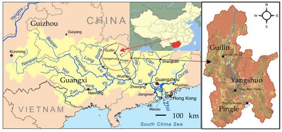
Figure 1.
Lijiang River situation and its three subbasins (Guilin, Yangshuo, and Pingle). The demographic Hu Line is presented in blue on the country map.
From the hilly and steep areas of north Guilin, which is part of the Maoershan Mountains, towards the flatter karstic landscapes of Yangshuo and Pingle counties (Figure 1) in the center and south, respectively, lies the famous Lijiang River with a total length of 214 km. As one of the eight tributaries of the well-known Pearl River in south China (Zhujiang in Chinese, the third largest river in the country), the Lijiang River plays a vital role in the watershed economy, transport, and drinking water supply. Lijiang has 13 tributaries and a total of 11,300 km2 catchment.
2.2. Methods Used
2.2.1. HEC-HMS Model and Its Extensions
In the present work, to forecast the flood and analysis and its influencing factors, the HEC-HMS model was employed to convert any targeted rainfall into runoff in the study area. The necessary input data about the watershed (such as morphology, shape, slope, area, types of land use, river network, soil types, etc.) and its weather (hydrometeorological data such as daily rainfall, humidity, air pressure, wind speed, etc.), as the primary input information to run the model, were provided from their receptive sources. Since HEC-HMS is a GIS (geographic information system)-based model, the required data were first embedded in some relevant software (extensions of the HEC-HMS) as different layers, such as digital elevation model (DEM) and river network (RN). For this purpose, the raster data of the DEM layer was downloaded from the USGS website (United States Geological Survey, https://earthexplorer.usgs.gov (accessed on 10 May 2022) as 30 m square mosaics to be used in an Arc-Hydro extension. The software helped to splice (connect) and crop (trim) the mosaics to obtain the watershed DEM layer in accordance with its boundaries and shape and obtain other required parameters such as the longest river length or the distance of each point to the catchment gravity center.
Later, the DEM layer was masked in HEC-GeoHMS (geospatial hydrologic modeling, another GIS-based software) to be eventually used in the HEC-HMS. The Universal Transverse Mercator (UTM) map of the study area, which assisted in categorizing the slope and specifying the flow directions of the tributaries, was used as another layer in Arc-Hydro. Via UTM, we located specific points of the watershed to coordinate with GIS, based on the zone (60 zones on the globe, 6° each longitude) where they are located; our study area is located in zone 49. Another necessary layer was the river network information as vector data; its shape files were downloaded from https://www.openstreetmap.org (accessed on 12 May 2022) before being trimmed via Arc-Hydro. For accuracy, the river network data was visually compared with various references such as existing actual maps of the watershed and Google Earth to calibrate the output since the topography of the watershed sometimes mistakenly assigned the low-level locations, paths, or valleys as river canals. Lastly, the watershed and its sub-watersheds were delineated in GIS through the HEC-GeoHMS to figure out the river length and other geometrical characteristics.
Landsat images of the study area for 2013 were obtained from GIM Cloud (a Chinese cloud platform for geographical information monitoring) to compute these areas and the CN numbers of the basin, taking into consideration the different types of land use. Through identifying specific colors for each type of land use, we categorized the various areas of the watershed as construction, wetland, river, grassland, woodland, cropland, etc. Having soil type information of the basin from the Food and Agriculture Organization (FAO) portal available at https://www.fao.org/soils-portal/data (accessed on May 2022), the SCS-CN numbers of the study area were pulled out via HEC-GeoHMS. The necessity of the CN number is to assign different rates of soil infiltration, classified according to the type of soil in different regions.
More than six decades (1954–2017) hydrometeorological data (rainfall, runoff, water level, etc.) from three stations (at the subbasins outlet including Guilin, Yangshuo, and Pingle) were acquired. The missing data were obtained via regression with a high value of R2, which showed a good correlation between the data. Rainfall values were geographically extended across the watershed via the zonal function of GIS. This function is in fact, a radial basis function or RBF, which showed how the gradient of the precipitation decreased from one side of the watershed to another (decreased from north to south in our case).
Another software used in this work was Hydrological Frequency Analysis Plus DSS or Hyfran-Plus. It was employed to compute the expected peak discharges for a wide range of return periods as low as 2 and as high as 10,000 years. The software uses a built-up technique which mathematically fits the statistical distribution of extreme events. The term DSS is the abbreviation for decision support system that assisted in selecting the best fitting distribution for the data being analyzed via applying the Weibul, Gumbel, and Gamma tests. The process was performed according to the null or alternate hypotheses, H0 or H1, of the accuracy of the tests. The abovementioned examinations were performed to assess if the result was statistically adequate and accurate at a certain significance level for reliable values of p (<0.05 α at 95% confident level) to decline the H0 or H1 acceptance.
To simulate the hydrograph of any rainfall in any watershed, we initially needed to produce the unit hydrograph based on the characters of that particular rainfall or basin. Among the known methods are the SCS and Snyder unit hydrograph (SUH). These mutually are the applied techniques to estimate the hydrograph prior to being considered in HEC-HMS. Considering the size of the study area for this work, the Snyder method was employed to simulate the unit hydrograph, and at the same time, the SCS method was used as control. To calculate, at the beginning, the maximum instantaneous discharge values were computed based on the average rates of the monthly discharges. Later, via Hyfran-Plus and using the annual maximum instantaneous discharge rates, the expected peak discharge in each sub-basin was computed. Finally, the graph for each sub-watershed was calculated via the SUH and SCS techniques (the related formulas are explained elsewhere) and amended based on the expected peak discharge (at various frequencies).
The calculated Snyder hydrograph provided special discharge values at certain times (such as peak time). Thus, the computed hydrograph was transformed into shorter time series (i.e., in an hour) using the regression for each limb of the hydrograph. Later, the obtained values of the hydrographs could be multiplied in desired precipitations (net values which are obtained by certain precipitations in certain return periods) to produce the flood hydrographs of those individual precipitations in their respective sub watersheds. Therefore, the six hours precipitation in various return periods (50 years in this study) in the 3 subbasins are computed in this case. Although the final model can forecast floods for any desired duration or frequency, these initial selections (6 h of rain and 50 years return period) are based on criteria such as the size of our study area, the available rainfall-runoff data, recorded flood events, the purpose in which the hydrograph is calculated for (i.e., regional flood protection), and so on. The Snyder method is, in some cases, not reliable in computing the hydrological features including the hydrograph’s base time or the peak time. Compared with the Hyfran-Plus calculated “expected peak-discharge” for any given return period, the amounts obtained by the unit in hydrograph methods will lead to an adapted graph to be paired with some marked floods in the basin. The required changes are mostly on the peak discharge rates and times for any given volume of runoff. Finally, the adapted graphs could be calibrated via HEC-HMS. Due to the use of simplified formulas as well as uncertainties in HEC-HMS as compared with the real scenarios, the estimations usually need post-processing and modification via confirming the results with actual rainfall-runoff events, and the computed amounts for the individual catchment.
Although HEC-HMS applied a unit hydrograph, it used the Muskingum technique for flood routing [10]. Dissimilar to the SCS or SUH, Muskingum considered the shape and features of the catchment components in the prism and wedge storage volume, known as the steady portion and the extra portion of the flow, respectively. Coefficients X and K were introduced for higher levels of sophistication and reliability in the peak flood calculation. In practice, the resulting form of the estimated hydrograph was influenced by several criteria. The correlation between these two (K and X which is dimensionless) has been presented below (Equation (1) and Figure 2):
in which the flow-specific gravity index X shows the weightage criteria for current segmentation to the wedge and prism, and K is an index showing the traveling time (propagation time) in h for the flow.
Storage volume = K (wedge + prism) = K [(X × inflow) + ((1 − X) × outflow)]
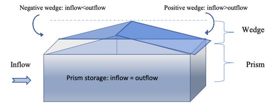
Figure 2.
Prism and wedge storage concepts, graphically.
As an example, for X = 0.2, if the wedge was 20% and the prism would be 80% of the total current volume. For the parameter K, technically, the higher the value, the longer it will take for the peak of the flood to travel in downstream, which means an attenuated peak with a lesser peak discharge rate as it travels. Between the two (X and K) in this method, the latest has higher effects on the graph form and its peak, however; a bigger X value resulted in an exponential magnitude of the wedge.
2.2.2. Dams on Lijiang River
Specific hydraulic details (such as location; catchment area; water storage area; annual water inflow; total, effective, and dead storage capacities; crest, and spillway types, length, width, and elevations; stage-storage curve; etc.) of the dams were provided from the Guilin Water and Resources Bureau and encoded into the model. The simulated hydrographs with and without the dams were obtained and analyzed. As of today, in total 4 big-size dams are operating on Lijiang upper reaches tributaries. Besides the Qingshitan reservoir, located in the Gantangjiang River (a northwestern tributary of the Lijiang River) which has been operating since 1961 with 600 million cubic meters of effective storage capacity, there are 3 smaller dams built on the northern tributaries in recent years. These three with a total combined capacity of 438 m3, are the Chuanjiang reservoir, built on the Chuanjiang tributary and operating since March 2014 with a total storage capacity of 98 million m3; the Xiaorongjiang reservoir, located in the Xiaorongjiang tributary and operating since January 2016, with a total storage capacity of 152 million m3; and lastly the Fuzikou reservoir, located in the Ludonghe tributary and operating since January 2018, with a total storage capacity of 188 million m3. These four reservoirs will supplement water to the Lijiang River in the dry season and can partially control the flood in the watershed during the wet season.
2.2.3. Soil Moisture Accounting Loss and the Use of Artificial Neural Network
Soil moisture accounting loss data of the watershed was acquired from WheatA (available at http://www.wheata.cn/ (accessed on 18 May 2022)) for 10 different locations distributed all around the basin (Figure S1, Supplementary Materials). The amount of water in m3/m3 in different depths of the soil (10, 40, 100, and 200 cm) daily for 1.5 years (January 2020 to June 2021) was monitored across the watershed. Although the points were scattered across the watershed, the data was found to be highly correlated with an R2 value close to 1, hence we decided to use 10 locations where more data could be collected. The analysis was to assess the changes and fluctuations during the time, together with the daily rainfall data, versus runoff, using artificial neural network. For this assessment, the rainfall data was obtained from the global precipitation measurement mission satellite (GPM) for the watershed to have a higher correlation with the soil moisture data (averagely) on a bigger scale since points were distributed across the basin. The Long Sort-Term Memory (LSTM) artificial neural network with Python programming was used to find the correlation between 3 indexes including precipitation, soil moisture fluctuation, and the discharge rate of the river at the catchment outlet. Finally, the LSTM outcomes as coefficients were applied to the model (similar to the source and sink function), considering the flood event time via real data to compare and calibrate the produced hydrograph for 3 flood events in 3 locations in the basin.
Moreover, the underground water utilization which might have an impact on the soil moisture was considered; however, it was not considered as it was negligible. In this watershed, due to abundant rainfall and surface water resources, the drinking and agricultural water were mostly extracted from the river and reservoirs, unless in a draught situation. Moreover, due to the karst landform, extraction of groundwater may cause the land to collapse and hence it is prohibited unless especial permissions are obtained. In fact, Guilin City has a single water source which is Lijiang River supplying through four municipal water supply plants. In the water source and supply planning projects, the Qingshitan and Jinling reservoirs in Lijiang basin upstream are the emergency water source for the watershed. Groundwater is suggested to be the second emergency water resource, as backup but that is not implemented yet. Here, the natural recharge of groundwater resource is 369 million m3/year, and the exploitable groundwater resource of it is 174 million m3/year but is not being extracted. There are 151 groundwater monitoring points to monitor the water level and its quality across the watershed. The below flowchart (Figure 3) presents the steps of the methods used in this work in brief.
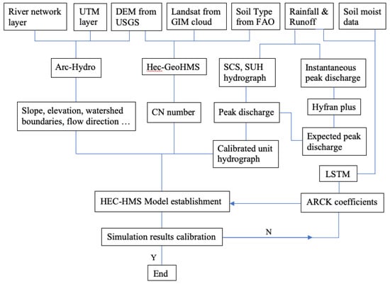
Figure 3.
Flowchart of the methods and extensions used in different stages to build the model.
3. Results
3.1. Initial Forecast via HEC-HMS
A total of nine model outputs were generated for three floods (May 2017, April 2018, and April 2019) in three subbasins’ outlets (Guilin, Yangshuo, and Pingle) to be calibrated versus the actual recorded data. The below hydrographs (two examples in Figure 4a,b) are the HEC-HMS simulated results for two individual flood events in Guilin and Yangshuo subbasins in 2018 and 2019. The actual graph (black color) in Figure 4b shows that one of the dams was released prior to an estimated heavy rainfall for flood control purposes. The simulated hydrographs are in blue. As can be seen, the graphs both have low accuracies. Even discarding the first bump in Figure 4b, which is the dam release peak, the second peak has not been estimated accurately by the model. A low NSE value (model efficiency coefficient) of −1.24 for Yangshuo (Figure 4b) shows the inaccuracy of the model in forecasting for this case, as for Guilin (Figure 4a), the NSE was 0.69. The Nash-Sutcliffe with a value of −∞ up to maximum 1 indicates the prediction power of the applied model. These initial results are prior to including the available reservoir capacity of karst (ARCK) as well as dams into the model.

Figure 4.
Actual (black) and simulated (blue) hydrographs of two floods (a) in Guilin during 19–22 April 2018 and (b) in Yangshuo station during 18–22 April 2019 before inclusion of ARCK and dams in the model.
3.2. ARCK Impact on Flood Formation
Figure 5 shows the river flow (in m3/s) fluctuations as a function of precipitation (in mm) and soil moisture loss during 1.5 years at the Guilin station outlet point. In fact, the positive or negative differences between these calculated values for the river discharge rate (shown in Figure 5) with the HEC-HMS predicted discharge values (before modification) are the Karst reservoir contribution into the total river discharge rates. These differences help to adjust the outflow in each subbasin based on the available reservoir capacity of karst (ARCK) translated from the soil moisture loss accounting which is a function of the amount of rainfall and its intervals. The same graph for the other two subbasins are presented in Supplementary Materials (Figures S2 and S3).
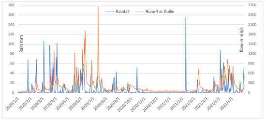
Figure 5.
River flow fluctuations in response to precipitation (and technically to the soil moisture) at Guilin subbasin.
3.3. Inclusion of Soil Moisture Accounting Loss for Model Modification
The Long Sort-Term Memory (LSTM) artificial neural network using python programming was applied to find the correlation between eight parameters to represent three indexes (precipitation, soil moisture, and river discharge rate). Soil moisture loss accounting data (averagely for the 10 given points to reduce the heterogenicity effect of soil types) in four different depths (10, 40, 100, and 200 cm as parameters 1–4) with GPM precipitation data (daily average for the watershed as parameter 5) versus river flow in three different locations of the watershed (as 6–8 input parameters) were analyzed using LSTM. The time in which the analysis was completed was 1.5 years (from 1 January 2020 to 31 June 2021). Soil moisture accounting loss data (parameters 1–4) versus precipitation (parameter 5) are presented below in Figure 6. As can be seen, the soil water content at different depths raises after each rainfall event and falls during the intervals. The longer the intervals, the lower the water content and vice versa.
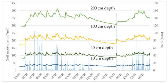
Figure 6.
Average daily soil moisture of 10 locations at different soil depths vs. rainfall in 1.5 years.
The fluctuations of the river flow and soil water content in response to the precipitation combined is presented for Guilin in the below graph (Figure 7). As can be seen, during the first 4 months of the year, since the soil water content is low, the major portion of the precipitations is percolated into the karstic network rather than causing any considerable raise in the river flow. In the following 3 months however, the river flow magnitude rose only after the ARCK reached its full capacity.
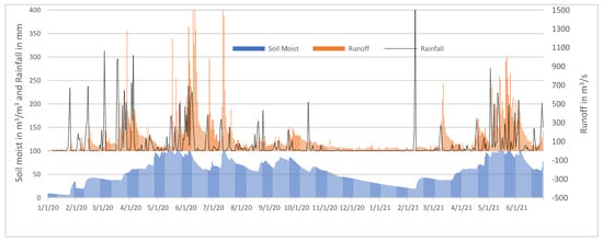
Figure 7.
Daily soil moisture and runoff vs. rainfall in Guilin for 1.5 years. Soil moisture values are −300.
As the correlation heatmap (produced by LSTM) in Figure 8a presents, the relationships between the 8 given parameters are shown using different colors in which the darker the color, the more significant the correlation between the two parameters.
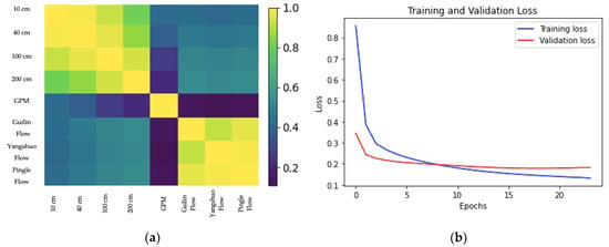
Figure 8.
(a) Feature correlation heatmap of the eight parameters via LSTM, darker colors show significant correlation. (b) Training and validation loss errors of the algorithm.
The correlation degrees (C) were orderly including significantly correlated 0 ≤ C < 0.2, correlated 0.2 ≤ C < 0.4, medium correlated 0.4 ≤ C < 0.6, weekly correlated 0.6 ≤ C < 0.8, and no correlation 0.8 ≤ C < 1. Numbers 1–8 show the eight introduced parameters (including 1–4 the soil water content at 10–200 cm depts, 5 the GPM precipitation, and 6–8 the flow in the three subbasins). As an example, flow in the second subbasin (Yangshuo as parameter 7) is significantly correlated with precipitation (dark color), correlated with the soil moisture, a weakly correlated with the Guilin flow (parameter 6), and shows no correlation with itself (yellow color) or the Pingle (parameter 8). Figure 8b shows the validation graph for the neural network algorithm error minimization. In this graph, lower amounts of loss show how accurate was the model prediction in which zero loss shows a perfect prediction. Epoch indicates the number of completed passes for the algorithm data set (24 epochs in our case).
3.4. Modified Model Outputs
After the inclusion of the soil moisture accounting loss and the dams into the model, the generated hydrographs were improved (Table 1). The nine simulated graphs of the floods were compared with actual data as well as with the initial model forecasts. Below two hydrographs (Figure 9a,b) are the given examples for the same events and locations (as in Figure 4) regenerated via the modified HEC-HMS. The simulated graphs in blue for both events have high similarities with their actual graphs in black. In Yangshuo, with a double peak hydrograph (in which the first bump is the dam release prior to an estimated heavy rainfall), both peaks were forecasted as we also included the dams in the model. The NSE values from −1.24 for Yangshuo and 0.69 for Guilin (Figure 4a,b) increased to 91% and 95%, respectively, which showed a high forecasting accuracy.

Table 1.
NSE values for the three simulated flood events (2017, 2018, and 2019) in Guilin (G) Yangshuo (Y) and Pingle (P) before and after LSTM modifications with ARCK and dams vs. initial simulations.
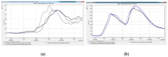
Figure 9.
Actual (black) and simulated (blue) hydrographs of a flood event in (a) Guilin in 19–22 April 2018 and (b) Yangshuo station in 18–22 April 2019 after LSTM modifications with ARCK and dams.
4. Discussion
As presented in Figure 4, the initial HEC-HMS results had low estimation accuracy which is due to the complexity of flow in porous environments. Karstic water transport is heavily dependent on the morphology, shape, pores and cracks size and distribution before it can join the free flow of the river or aquifers. The diversity of water movement (or its detention in underground lakes, caves, and rivers) and the probabilities from the unsaturated and epikarst zone to the saturated zone, (such as through the sinkholes and sky windows, shafts, surface runoff, loos sediment, and stone leaching) show how rainwater can go through different pathways in various current speeds which will have different lag times from short to long as compared with non-karst catchments. Conical hills, as presented in Figure 10a, will feed the river and underground aquifers as in abovementioned pathways. Besides these egg-box shape topographies, the covered karst (hidden under soil or sometimes loose sediment) in this watershed (Figure 10b) helps to feed the underground saturated soil layer through leaching in lower flow speeds depending on the bed’s hydraulic conductivity and infiltration rates [3]. These complexities posed by the specific physiological conditions of such basins are required to be quantitatively taken into consideration for reliable model forecasting. Therefore, modifications of the model results in the soil moisture accounting loss data via applying different tools.
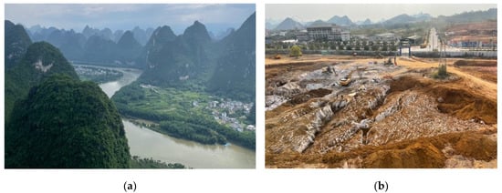
Figure 10.
Conical shape karst around Yangshuo (a), a typical covered karst area in Lijiang River watershed (b).
The “monsoon climate formed” karst in Guangxi consists of Fengcong (commonly based mountains) and Fengling (solitary mountains on intermountain plains) types. In terms of classification, it is in fact a zonal static type of karst, old (monadnock) and developed, due to the subtropical climate [32]. According to the evolution stage, karst can be in juvenile, youthful, mature, complex, extreme, and old stages. In the old stage, where the Guangxi karst is, the drainage networks (including cracks, dolines underground streams, caves, etc.) are well developed and the river flows in a relatively stable riverbed [33]. Hence, the inclusion of the soil moisture accounting loss should have a steady (during time) impact on flood formation for certain precipitations (in terms of intensity, duration, and return period). This requires us to monitor the soil water content (or technically ARCK) and rainfall intervals as a major contributor to the flood [23].
Unlike HEC-HMS results in non karst environments [34,35], the huge gap between the model estimations before (Figure 4a,b) and after (Figure 9a,b) the inclusion of soil moisture accounting loss indicates the importance of the ARCK in karst hydrology. The model’s initial runs showed a significant sensitivity to initial abstraction. As presented, when there were more frequent precipitations in the wet season (i.e., May and June 2020 in Figure 5), relatively small amounts of rain (40–60 mm) caused a drastic raise in the river flow (1900–2700 m3/s), that is because the ARCK was low or there was less available capacity left to store the rainwater. The response of the river flow during the dry season, however (i.e., Nov 2020 to Mar 2021 in Figure 5), is totally different in which even 172 mm rain within 2 days in early Feb 2021 did not produce any considerable rise in water flow (extra 23 m3/s only) since most of this stormwater sank into the karst network to fill the empty spaces of the high ARCK. Therefore, the magnitude of the ARCK could impact the occurrence and magnitude of floods in karstic areas. This was reflected in Mo et al.’s research [10] as the difference between the light and heavy rainfalls in which karstic’s free or pressured orifice outflows, respectively, will control the flood magnitude. In other words, a heavy rainfall will slow down the contribution rate of the karstic flow as in pressured orifices. This partially answers the question about why karstic flood predictions are inaccurate. However, what this work adds is that the ARCK, which is controlled by rainfall intervals, is mainly behind this phenomenon. Technically, how much of the total hidden reservoir’s capacity (as the primitive destination of the rainwater) is available will determine how much stormwater can be left to flow into the river. Comparing the two histograms presented in Figure 5 and Figure 6, and as combined in Figure 7 where river flow and soil water content for the same period will differently fluctuate in response to the precipitation, conceptually illustrates this phenomenon. Therefore, we saw in these two graphs that a heavy rainfall after a long interval was majorly stored in the karst’s empty spaces (Figure 6), while smaller rainfalls in the wet season did cause floods (Figure 5). Although the coefficients driven from the 1.5 years of recorded soil moisture data were applicable to the model output calibration for the few analyzed flood events in our case, these coefficients will vary since the rainfall patterns, intervals, temperature (which impacts the evapotranspiration), and other variables will fluctuate during different years. Hence, this indicates that we must consistently monitor the soil moisture for coefficient adjustment to continue having a more accurate, reliable, and updated prediction for future floods.
In terms of soil moisture, as illustrated in Figure 6, the response of the soil water content to the rain in deeper layers is proportionally less, with lower reoccurrence frequency, and in slower rates compared to the top layers. For instance, from 16 October 2020 to 31 January 2021 which was the longest interval of the dry season (discarding a few small rainfalls), the water content was reduced from 37.12 to 26.75 which is a 28% moisture loss; while there was a 200 cm decrease between 21 October 2020 and 9 February 2021 from 354.65 to 307.38, which is a 13.3% reduction. Another point observed was that the soil moisture fluctuation had a higher lag time at the lower depths. As in the abovementioned example, the water content at the 200 cm depth begin to decline 4 days after it was started at the 10 cm depth at the beginning of the dry season and continued to decline 9 days after the water content at 10 cm depth begin to raise at the end of the dry season. Moreover, the fluctuation occurrences at the shallow soil layers was more frequent than in deep soil, in which any small rainfall might cause saturation at the 10 cm depth while it may not impact the gradient trend at the 200 cm depth. Thus, we can see a continuous upward trend for 200 cm soil moisture from 25 January to 17 February 2020; while, at the 10 cm depth the water content fluctuated three times during this period.
In this work a total of 27 simulations on three flood events (May 2017, April 2018, and April 2019) were analyzed at three stations before and after the ARCK and dam inclusions. As shown in Table 1, the model output NSE values of these three floods were enhanced after ARCK was added to the model, as compared with simulations done after dams were included. While initial simulations’ NSE values were generally low, results revealed a 16% (averagely) NSE improvement after the inclusion of soil moisture accounting in the model compared with the after the dams’ inclusions (from average NSE of 0.65 to 0.81). This improvement indicates that the soil moisture loss accounting data can represent the available reservoir capacity of karst which drives the peak magnitude of floods in karstic watersheds, and therefore, can be used to improve HEC-HMS simulations in such basins. Furthermore, from the correlation heatmap in Figure 8a we could understand that besides the rainfall (parameter 5 as GPM) which was significantly correlated with the flow in the 3 subbasins (parameters 6 to 8), the soil moisture, as the second important parameter, has also a relatively strong correlation with the flow in which the shallower the dept of the soil, the more significant the correlations were. This indicates that this topsoil moisture can be translated into runoff more quickly (than the deep soil moist), and hence, when the ARCK is low (which means the karst reservoir is full) then the entire rainfall can be converted to runoff since no room for retention is left. Therefore, it makes sense to use the soil moisture as representative of the ARCK. Similarly, in southern France, karst initial state was found to have significant karst contribution into the flow [36].
Overall, the potential flood occurrence of certain rainfall is a function first of rainfall (taking into consideration its intensity and duration), and second the available reservoir capacity of karst at that particular time which depends on the total capacity and the precipitation intervals that assign the ARCK. This underpins the importance of soil water content monitoring and post-processing, especially at the topsoil and rout zones, for flood prediction accuracy. Besides the percolation to deeper layers, underground rivers, or aquifers, the evapotranspiration will also extract water from the soil, like a canopy model [37]. These two phenomena as influencing factors will control the ARCK during the intervals. Hence, in future research on the ARCK, evapotranspiration must also be included for the intervals when we calculate the coefficients to modify the model simulations, more accurately, as this is an active area of research.
5. Conclusions
This work has conducted HEC-HMS model modification through the inclusion of soil moisture accounting loss as an indicator of available reservoir capacity of karst (ARCK) for the Lijiang River flood forecasting. In this study, we did use the artificial neural network to link the 1.5 years of soil moisture accounting loss data to the river discharge rate which contributes to the flood. The Long Sort-Term Memory (LSTM) artificial neural network was used to pull out ARCK coefficients which can adjust the river discharge rates based on rainfall-runoff data and intervals. Depending on the time intervals between the rainfall events, the karst reservoir capacity fluctuates, and this will impact how much of rain can be immediately converted into runoff and what portion can be held in karst cracks and caves to fill the karst reservoir capacity. As an example, 21 mm/d of rain during 4 days in the wet season increased the river discharge rates from 10 to 20 times greater than before; however, 87 mm/d of precipitation in 2 days at the end of the dry season only caused a raise from 0.1 to 0.64 on the current at different stations. This was reflected by soil water content monitoring at various depths from 10 to 200 cm. The heat map produced via Python programming showed that the river water level was correlated with the soil moisture after precipitation. Using this technique we could modify the HEC-HMS results for individual flood events in which the simulated results were much closer to the actual flood data compared to the original model forecasting. NSE values of the simulated hydrographs which were initially not accurate, improved by 16%, averagely, after the inclusion of soil moisture accounting data into the model compared with simulations done after dams were included. Therefore, we recommend observing and monitoring the soil water content, as an important driver, to continuously have updated data for hydrological model prediction calibration of future floods in this watershed.
Supplementary Materials
The following supporting information can be downloaded at: https://www.mdpi.com/article/10.3390/atmos13101544/s1, Figure S1: Locations of the collected soil moisture data across the watershed; Figure S2: River flow fluctuations in response to the soil moisture accounting loss and precipitation at Yangshuo subbasin; Figure S3: River flow fluctuations in response to the soil moisture accounting loss and precipitation at Pingle subbasin.
Author Contributions
J.D. conceptualization, editing, supervision; S.R. methodology, writing the original draft; J.X. data curation and writing and review; Z.W. investigation, and visualization; Z.L. and L.P. formal analysis, project administration, and resources; A.S. validation, software. All authors have read and agreed to the published version of the manuscript.
Funding
This work was funded by the Natural Science Foundation of China (Grant No. 52150410408, No. 51979046), the National Key Research and Development Program of China (Grant No. 2019YFC0507500), the Science and Technology Major Project of Guangxi, China (Grant No. AA20161004).
Institutional Review Board Statement
Not applicable.
Informed Consent Statement
Not applicable.
Data Availability Statement
Not applicable.
Acknowledgments
The authors wish to thank the reviewers for their constructive comments.
Conflicts of Interest
The authors declare no conflict of interest.
References
- Zhang, J.; Huan, X.; Lu, H.; Wang, C.; Shen, C.; He, K.; Lu, Y.; Wu, N. Crossing of the Hu line by Neolithic population in response to seesaw precipitation changes in China. Sci. Bull. 2022, 67, 844–852. [Google Scholar] [CrossRef]
- Liu, J.; Shi, Z. Quantifying land-use change impacts on the dynamic evolution of flood vulnerability. Land Use Policy 2017, 65, 198–210. [Google Scholar] [CrossRef]
- Jiang, G.; Guo, F.; Tang, C. Groundwater systems in bare and covered karst aquifers: Evidence from tracer tests, hydrochemistry, and groundwater ages. Environ. Earth Sci. 2019, 78, 608. [Google Scholar] [CrossRef]
- Willenbrink, E. Policy Communication and the Influence of Agricultural Communities on Karst Landscapes: A Case Study in Phong Nha-Kè Bàng National Park, Vietnam. Master’s Thesis, Western Kentucky University, Bowling Green, KY, USA, 2018. Paper 2076; Specialist Projects. Available online: https://digitalcommons.wku.edu/theses/2076 (accessed on 1 February 2022).
- Jiang, G.; Guo, F.; Wei, M. Hydrogeological characteristics of foot caves in a karst peak-forest plain in South China. Hydrogeol. J. 2020, 28, 535–548. [Google Scholar] [CrossRef]
- Choudhury, P.; Shrivastava, R.K.; Narulkar, S.M. Flood routing in river networks using equivalent Muskingum inflow. J. Hydrol. Eng. 2002, 7, 413–419. [Google Scholar] [CrossRef]
- Dastorani, M.T.; Khodaparast, R.; Talebi, A.; Vafakhah, M.; Dashti, J. Determination of the ability of HEC-HMS Model components in rainfall-run-off simulation research. J. Environ. Sci. 2011, 5, 790. [Google Scholar]
- Kabeja, C.; Li, R.; Guo, J.; Rwatangabo, D.E.R.; Manyifika, M.; Gao, Z.; Wang, Y.; Zhang, Y. The Impact of Reforestation Induced Land Cover Change (1990–2017) on Flood Peak Discharge Using HEC-HMS Hydrological Model and Satellite Observations: A Study in Two Mountain Basins, China. Water 2020, 12, 1347. [Google Scholar] [CrossRef]
- Sharafati, A.; Khazaei, M.R.; Nashwan, M.S.; Al-Ansari, N.; Yaseen, Z.M.; Shahid, S. Assessing the Uncertainty Associated with Flood Features due to Variability of Rainfall and Hydrological Parameters. Adv. Civ. Eng. 2020, 7948902. [Google Scholar] [CrossRef]
- Mo, C.; Wang, Y.; Ruan, Y.; Qin, J.; Zhang, M.; Sun, G.; Jin, J. The effect of karst system occurrence on flood peaks in small watersheds, southwest China. Hydrol. Res. 2021, 52, 305–322. [Google Scholar] [CrossRef]
- Delphi, M.; Shooshtari, M.M.; Zadeh, H.H. Application of Diffusion Wave Method for Flood Routing in Karun River. Int. J. Environ. Sci. Dev. 2010, 1, 432. [Google Scholar] [CrossRef]
- Tewolde, M.H.; Smithers, J. Flood routing in ungauged catchments using Muskingum methods. Water SA. 2006, 32, 379–388. [Google Scholar] [CrossRef]
- Zhang, H.L.; Wang, Y.J.; Wang, Y.Q.; Li, D.X.; Wang, X.K. The effect of watershed scale on HEC-HMS calibrated parameters: A case study in the Clear Creek watershed in Iowa, US. Hydrol. Earth Syst. Sci. 2013, 17, 2735–2745. [Google Scholar] [CrossRef]
- Nyaupane, N.; Mote, S.R.; Bhandari, M.; Kalra, A.; Ahmad, S. Rainfall-runoff simulation using climate change-based precipitation prediction in HEC-HMS Model for Irwin Creek, Charlotte, North Carolina. In Watershed Management, Irrigation and Drainage, and Water Resources Planning and Management, Proceedings of the World Environmental and Water Resources Congress, Minneapolis, MN, USA, 2018; American Society of Civil Engineers: Reston, VA, USA, 2018; pp. 352–363. [Google Scholar]
- Şen, Z. General modeling of karst spring hydrographs and development of a dimensionless karstic hydrograph concept. Hydrogeol. J. 2020, 28, 549–559. [Google Scholar] [CrossRef]
- Şen, Z.; Dabanlı, İ.; Şişman, E. Physical and practical hydrograph recession modeling in karstic sinkholes. Water Supply 2020, 20, 751–760. [Google Scholar] [CrossRef]
- Zhou, Q.; Chen, L.; Singh, V.P.; Zhou, J.; Chen, X.; Xiong, L. Rainfall-runoff simulation in karst dominated areas based on a coupled conceptual hydrological model. J. Hydrol. 2019, 573, 524–533. [Google Scholar] [CrossRef]
- Vereecken, H.; Schnepf, A.; Hopmans, J.W.; Javaux, M.; Or, D.; Roose, T.; Vanderborght, J.; Young, M.H.; Amelung, W.; Aitkenhead, M.; et al. Modeling soil processes: Review, key challenges, and new perspectives. Vadose Zone J. 2016, 15, vzj2015.09.0131. [Google Scholar] [CrossRef]
- Ghazanfari, S.; Pande, S.; Cheema, M.J.M.; Alizadeh, A.; Farid, A. The role of soil moisture accounting in estimation of soil evaporation and transpiration. J. Hydroinformatics 2016, 18, 329–344. [Google Scholar] [CrossRef]
- Wang, D. A new probability density function for spatial distribution of soil water storage capacity leads to the SCS curve number method. Hydrol. Earth Syst. 2018, 22, 6567–6578. [Google Scholar] [CrossRef]
- Li, R.; Chen, Q.; Tonina, D.; Cai, D. Effects of upstream reservoir regulation on the hydrological regime and fish habitats of the Lijiang River, China. Ecol. Eng. 2015, 76, 75–83. [Google Scholar] [CrossRef]
- Zeng, C.; Guo, C.; Hu, J. Researches on variation in water resources of up reaches of Lijiang River. Resour. Environ. Eng. 2005, 19, 203–207, (In Chinese with English Abstract). [Google Scholar]
- Huang, W. Spatial dimensions of tower karst and cockpit karst: A case study of Guilin, China. Ph.D. Thesis, The University of Wisconsin-Milwaukee, Milwaukee, WI, USA, 2014; p. 54. Available online: https://dc.uwm.edu/etd/626 (accessed on 25 May 2022).
- Rad, S.; Dai, J.; Xu, J.; Wan, Z.; Zitao, L.; Linyan, P. Lijiang Flood Characteristics and Implication of Karst Storage Through Muskingum Flood Routing Via HEC-HMS, S. China. Hydrol. Res. 2022, in press. [Google Scholar]
- Cao, Y.; Zhang, J.; Yang, M.; Lei, X.; Guo, B.; Yang, L.; Zeng, Z.; Qu, J. Application of SWAT Model with CMADS Data to Estimate Hydrological Elements and Parameter Uncertainty Based on SUFI-2 Algorithm in the Lijiang River Basin, China. Water 2018, 10, 742. [Google Scholar] [CrossRef]
- Xu, J.; Dai, J. Variation characteristics of runoff in upper reaches of Lijiang River basin. Yangtze River 2018, 49, 41–46, (In Chinese with English abstract). [Google Scholar]
- Qi, J.; Xu, M.; Cen, X.; Wang, L.; Zhang, Q. Characterization of Karst Conduit Network Using Long-Distance Tracer Test in Lijiang, Southwestern China. Water 2018, 10, 949. [Google Scholar] [CrossRef]
- Mao, X.; Meng, J.; Wang, Q. Modeling the effects of tourism and land regulation on land-use change in tourist regions: A case study of the Lijiang River Basin in Guilin, China. Land Use Policy 2014, 41, 368–377. [Google Scholar] [CrossRef]
- Yao, Y.; Mallik, A. Stream Flow Changes and the Sustainability of Cruise Tourism on the Lijiang River, China. Sustainability 2020, 12, 7711. [Google Scholar] [CrossRef]
- Guizhen, H.; Xiang, Z.; Mingzhao, Q.Y. Exploring the multiple distribution of karst landscape in Guilin World Heritage Site, China. Catena 2021, 203, 105349. [Google Scholar] [CrossRef]
- Dai, J.; Rad, S.; Xu, J.; Pen, S.; Gan, L.; Chen, X.; Yu, C.; Zhang, S. Impacts of Climate Change Versus Landuse Change on Recent Lijiang River Flood Regime, South China. Tecnol. Y Cienc. Del Agua 2021, 12, 257–303. [Google Scholar] [CrossRef]
- Veress, M. Karst types and their karstification. J. Earth Sci. 2020, 31, 621–634. [Google Scholar] [CrossRef]
- Jia, Z.; Liu, X.; Cai, X.; Xing, L. Quantitative Remote Sensing Analysis of the Geomorphological Development of the Lijiang River Basin, Southern China. J. Indian Soc. Remote Sens. 2019, 47, 737–747. [Google Scholar] [CrossRef]
- Brirhet, H.; Benaabidate, L. Comparison of Two Hydrological Models (Lumped and Distributed) Over A Pilot Area of The Issen Watershed in The Souss Basin, Morocco. Eur. Sci. J. ESJ 2016, 12, 347. [Google Scholar] [CrossRef][Green Version]
- Tassew, B.G.; Belete, M.A.; Miegel, K. Application of HEC-HMS model for flow simulation in the lake tana basin: The case of gilgel abay catchment, upper blue nile basin, Ethiopia. Hydrology. 2019, 6, 21. [Google Scholar] [CrossRef]
- Bailly-Comte, V.; Jourde, H.; Roesch, A.; Pistre, S.; Batiot-Guilhe, C. Time series analyses for karst/river interactions assessment: Case of the Coulazou river (southern France). J. Hydrol. 2008, 349, 98–114. [Google Scholar] [CrossRef]
- Van der Tol, C.; Verhoef, W.; Timmermans, J.; Verhoef, A.; Su, Z. An integrated model of soil-canopy spectral radiances, photosynthesis, fluorescence, temperature and energy balance. Biogeosciences 2009, 6, 3109–3129. [Google Scholar] [CrossRef]
Publisher’s Note: MDPI stays neutral with regard to jurisdictional claims in published maps and institutional affiliations. |
© 2022 by the authors. Licensee MDPI, Basel, Switzerland. This article is an open access article distributed under the terms and conditions of the Creative Commons Attribution (CC BY) license (https://creativecommons.org/licenses/by/4.0/).