Electromagnetic Induction Measurements for Investigating Soil Salinization Caused by Saline Reclaimed Water

Abstract

This paper focused on the use of electromagnetic induction measurements in order to investigate soil salinization caused by irrigation with saline reclaimed water. An experimental activity was carried out during the growing season of tomato crop in order to evaluate expected soil salinization effects caused by different saline agro-industrial wastewaters used as irrigation sources. Soil electrical conductivity, strictly related to the soil salinity, has been monitored for three months by means of Electromagnetic Induction (EMI) measurements, and evident differences in the soil response have been observed. The study highlighted two aspects that can improve soil investigation due to the utilization of geophysical tools. First, EMI data can map large areas in a short period of time with an unprecedented level of detail by overcoming practical difficulties in order to massively sample soil. At the same time, repeated measurements over time allow updating real-time soil salinity maps by using accurate correlations with soil electrical conductivity. This application points out how integrated agro-geophysical research approaches can play a strategic role in agricultural saline water management in order to prevent soil salinization risks in medium to long-term periods.

1. Introduction

Irrigated agriculture is the main user of water in Europe and plays a pivotal role in the European economic contest. Water scarcity regions, such as the Mediterranean region, require innovative and sustainable approaches to enhance the use of non-conventional water sources in agriculture as a component of effective water conservation strategies. In this context, the use of municipal or agro-industrial wastewaters (AIW) is acquiring ever increasing interest and importance, particularly for irrigation in agriculture, which is the most water demanding economic sector worldwide. Reclaimed water is considered a non-expensive and reliable source; nutrients and organic matter present in this water can result in benefits for both crops, soils and the economy of the growers because it can reduce the use of synthetic chemical fertilizers. Even low water scarcity locations, such as northern Europe, water reclamation is becoming an attractive solution for environmental protection purposes because it can save freshwater by reducing groundwater over-exploitation and replenish over-exploited aquifers by acting such as a managed aquifer recharge system. Inappropriate water reclamation and mismanagement in its reuse may, however, result in negative impacts for both human health and environment. In addition, in some areas of the Mediterranean region [1,2], soil fertility may be affected by salt and heavy metals accumulation with serious degradation of soil quality and health in medium to long-term periods. The need for affordable, efficient and reliable water reclamation reuse has, therefore, become imperative. In light of these considerations, large-scale monitoring of the main changing factors in microclimate, such as crop water requirements, crop and soil parameters and soil water dynamisms, is needed in order to adequately estimate reclaimed water-use efficiency in the context of irrigation water management for sustainable agro-system production and as actions for tackling climate changes.

Typical sensors commonly used in agriculture (TDR, TDT and CE probes) provide local measurements of the soil properties and cannot capture the heterogeneities of the soil. On the other hand, it is unrealistic to install a high number of sensors both on the surface and in depth to cover large areas. In this regard, geophysical measurements can be used for agricultural purposes as a proxy for assessing spatial variability in soil properties because they are sensitive to soil moisture and salinity, as well as soil texture and composition properties [3,4]. In the last decade, geophysical data, particularly electrical and electromagnetic data, have been increasingly used to map soil drainage [5,6]; to characterize soil structure [7,8]; to detect soil–rock interface [9]; to map soil moisture [10,11]; to evaluate spatial variability of root water uptake [12,13,14,15,16]; and to quantify root biomass [17,18]. In particular, electromagnetic measurements have proved to be a useful tool for soil monitoring because the measured parameter, i.e., the apparent electrical conductivity (σ_a or ECa), is strictly related to soil salinity. Unlike the aforementioned sensors or traditional DC electrical survey, its noncontacting nature makes it a powerful tool for the measurement of soil electrical conductivity both on local and regional field scales. In fact, data acquisition is very fast because the operator moves the sensors during acquisition, allowing a collection of a large amount of data over wide areas by only walking through the fields.

Furthermore, the design of the modern multi-coil electromagnetic systems allows for the simultaneous collection of apparent electrical conductivity (ECa) data at different depths, increasing the capability to acquire measurements in a relatively short period of time. Although ECa is the equivalent electrical conductivity of a homogeneous half-space that produces the same measured response to the instrument in a single configuration, several case studies demonstrated that ECa is effectively correlated to soil salinity through different calibration approaches [19,20,21,22,23]. On the other hand, according to the classical geophysical inversion theory, the inversion of multi-configuration electromagnetic data represents a rigorous numerical approach in producing a robust model of electrical conductivity distributions on the investigated subsoil layer [24,25,26,27,28]. Regardless of the used approach for the data processing, the feasibility of collecting a large amount of the soil salinity data over wide areas by using noninvasive electromagnetic induction measurements can represents a powerful tool for evaluating the impact of different water qualities on soil properties. In addition, the capability of periodically repeating geophysical measurements can provide a significant advantage in understanding soil processes compared with the traditional point scale measurements and sampling. These two key factors of the geophysical prospecting have been highlighted in the present study, where the effects on the application of a nonconventional agricultural practice have been tested by using a multi-scale approach. In fact, in an experimental farm located in Southern Italy irrigated with two different reclaimed wastewaters and with freshwater, soil salinity has been inferred via time-lapse electromagnetic measurements and compared by using soil sample analysis.

The aims of the study were as follows: (i) to assess the reliability of the large-scale EMI data as alternative or support to traditional soil investigation methods; (ii) to correlate ECa distribution with soil electrical conductivity through an appropriate site-specific calibration function; and (iii) to explore the use of the noninvasive time-lapse electromagnetic survey as a real time monitoring tool for evaluating the impact of different water quality on soil salinity over the irrigation season.

2. Materials and Methods

2.1. Site Description

This experiment was conducted in 2020 (April to September) in the northern part of Apulian Region on a tomato orchard (Lycopersicon esculentum Mill.) cultivar Manyla (Semillas Fitó, Spain). Tomato plants were covered with an anti-hail net and grown in a net house structure. The tomato orchard was located at the Fiordelisi food manufacturing company (41.2431 N–15.7134 E WGS UTM84, altitude 160 m asl), which produces and processes different vegetables. The main climatic parameters recorded from the gauge station located near the experimental site during the growing season of the tomato, from April to September, are reported in

Table 1. Climatic parameter recorded during the irrigation season of the tomato during 2020 in the Stornarella gauge station.

Growing Season Month	Tomato 2020 April	May	June	July	August	September
Climatic parameter a
TMAX (°C)	28.7	36.3	38.5	40.6	41.7	35.6
TMIN (°C)	−0.6	7.3	11.9	13.2	16.2	9.4
TAVERAGE (°C)	14.6	20.1	23.2	26.2	28.0	23.9
Ra (MJ m−2 d−1)	34.5	39.71	41.7	40.4	35.9	28.9
ETo (mm)	121.1	169.5	186.4	205.8	190.9	127.7
P (mm)	42.6	35.2	15.4	41.6	20.2	35.8

^a T_MAX, T_MIN and T_AVERAGE—maximum, minimum and average air temperature; Ra, extraterrestrial solar radiation; ETo, reference evapotranspiration; P, precipitation.

. Total precipitation occurred in 2020 was 434 mm. Total precipitation occurred during the irrigation season (from April to the beginning of September) was 155 mm. The highest mean value of air temperature was detected during August; moreover, the highest Eto value was detected during July.

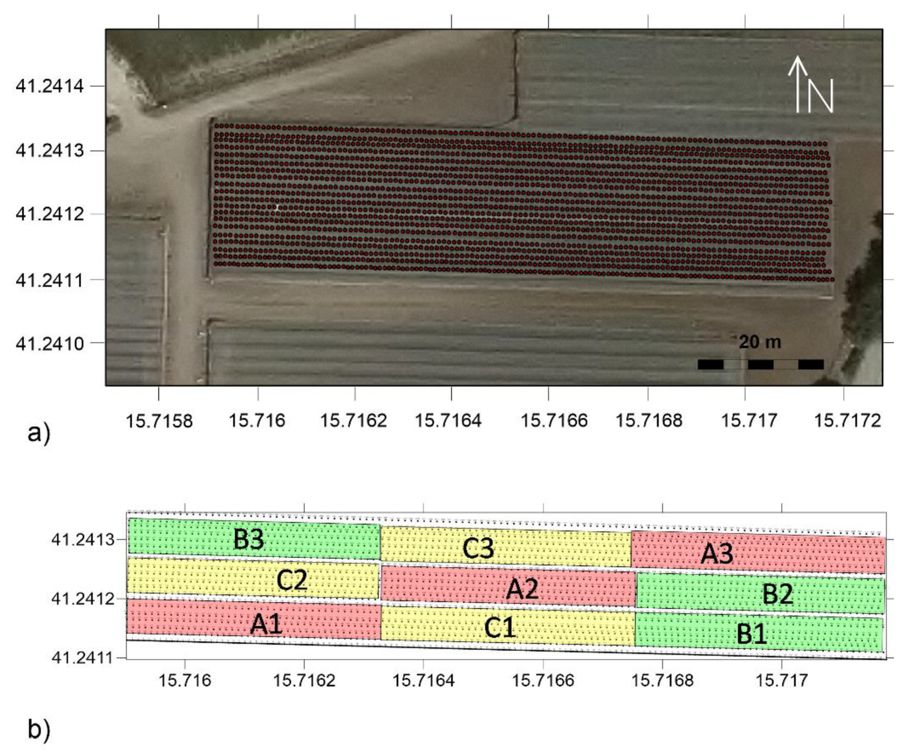
Three different irrigation treatments were compared: fresh water (FW) + conventional fertigation (plots A); Agro-industrial wastewater (AIW) + conventional fertigation (plots B); AIW + smart water fertigation (plots C). The experimental area, of about 3000 m², was divided into nine plots (A1, A2, A3, B1, B2, B3, C1, C2 and C3) so that each treatment had three replicates (Figure 1).

Fertilizer application rates of A, B and C plots were calculated according to potential yield and soil chemical characteristics. Moreover, fertilizer application rates of C plots were calculated by considering valuable plant nutrients of AIW. Before transplanting, a granular fertilizer in planting rows was distributed. After transplanting, dissolved fertilizers were supplied by fertigation technique through the irrigation system. Each treatment was equipped by a venture-type injector, and water-soluble fertilizers were injected with water in-line drippers at weekly intervals. Pre-transplanting, fertilizers were applied to the soil in all investigated plots by distributing 30 kg ha⁻¹ N and 35 kg ha⁻¹ P. Throughout the crop cycle, for plot A and B, 75 kg ha⁻¹ N, 40 kg ha⁻¹ P and 72.5 kg ha⁻¹ K were added by using fertigation. On the other hand, 75 kg ha⁻¹ N and 40 kg ha⁻¹ P were added by using fertigation in plot C.

Table 2. Chemical parameters for both fresh water (FW) and Agro-Industrial wastewater (AIW). Each data represent the mean of 11 values ± the standard deviation measured on water samples collected during the 2020.

Parameters	FW	AIW	t-Test
pH	7.3 ± 0.06	7.3 ± 0.01	n.s.
EC (µS/cm)	497.6 ± 38.7	2236.6 ± 218.8	***
Na (mg/L)	33.9 ± 3.2	359.3 ± 40.8	***
Cl− (mg/L)	48.7 ± 4.4	538.6 ± 64.7	***
SAR	1.2 ± 0.1	13.3 ± 1.4	***
Ca (mg/L)	48.9 ± 3.5	41.5 ± 4.4	n.s.
Mg (mg/L)	7.5 ± 0.90	8.2 ± 2.3	n.s.
K (mg/L)	9.0 ± 0.9	62.9 ± 8.4	***
P (mg/L)	0.05 ± 0.02	1.7 ± 0.4	*
NO3− (mg/L)	61.2 ± 9.0	5.3 ± 4.5	***

Note: Statistically significant at p-value significance level: * 0.05, ** 0.01, *** 0.001 levels of significance. n.s. means not significant.

shows the physico-chemical characteristics of water sources used in the test.

The experiment was conducted in sandy clay loam soil (sand 52%; clays 34%; silt 14%): hapoxeralf-argixeroll soil for USDA classification. Soil characteristics are reported in

Table 3. Soil characteristics.

Parameters	Value	Unit Measure
Total limestone	6.2 ± 0.9	%
Active limestone	3.9 ± 0.6	%
Calcium	28.5 ± 2.9	meq/100 g
Magnesium	10.9 ± 1.4	meq/100 g
Potassium	1.7 ± 0.2	meq/100 g
Sodium	2.1 ± 0.4	meq/100 g
Cation exchange capacity	43.3 ± 7.8	meq/100 g
Organic carbon	0.7 ± 0.05	%
Organic matter	1.2 ± 0.1	%
Total nitrogen	2.0 ± 0.3	‰
ECe	0.6 ± 0.1	mS/cm
pH	7.6 ± 0.1

. Tomato seedlings were transplanted into the plots on 5 April 2020 in mulched paired rows (40 cm apart) spaced at 250 cm, with plants at a distance of 30 cm apart along each single row. The final plant density was 2.7 plants m^–2. The plants were grown in a vertical setting, using nylon threads disposed between plant collars, and iron wires arranged longitudinally in the direction of the plant rows and fixed to the upper part of the net-house at 2.5 m from the ground. All plots were irrigated at the same time by using an automatic irrigation system. Each treatment was supplied by mean a water flow meter. All treatments received the same amount of water. The total amount of water used during the irrigation season was 4850 m³ ha⁻¹. In this study, irrigation was conducted by maintaining the soil water content (SWC) of the first 40 cm of soil in an optimum range between field capacity and allowable soil water depletion by using real-time soil moisture probes for continuous soil monitoring (TEROS 12). In particular, field capacity and the refill point (RP) were 32% and the 28%, respectively.

2.2. Basics of Electromagnetic Induction

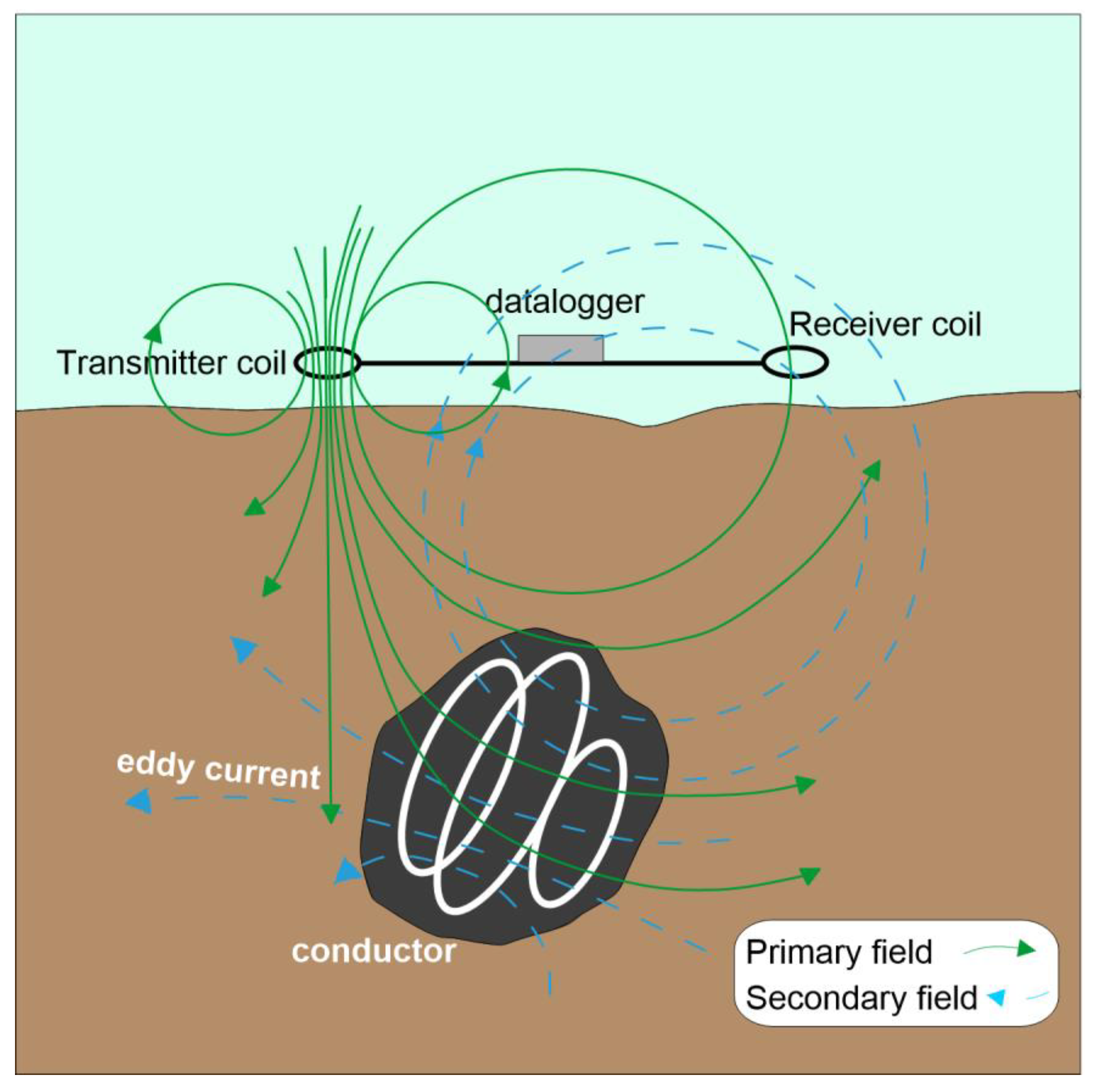
The electromagnetic Induction (EMI) technique, also called Frequency Domain Electromagnetics (FDEM), is based on the induction of electrical currents in the conductive subsurface through electromagnetic waves generated on the surface. A simple description of the basics is shown in Figure 2. A transmitter coil generates an alternate current that spreads into the subsurface. As electromagnetic (EM) waves travel through different materials, eddy currents induce secondary EM fields. At the surface, a receiver coil records a signal that is the sum of the primary and secondary field.

The components of the secondary field that are in-phase with the primary transmitted field and portion, which is 90-degrees out of phase (the quadrature component), are measured by a data logger. Under normal subsurface conditions, the in-phase component is strongly affected by the presence of buried metallic objects, while the quadrature component is directly related to subsurface conductivity [29].

The electromagnetic properties of the medium affect the depth of investigation of an EM system.

In fact, the depth of penetration of a signal, defined as skin depth δ, is obtained from the following:

$$\delta =\sqrt{\frac{2}{\sigma \mu \omega }}$$

(1)

where σ is the half-space conductivity, µ is magnetic permeability and ω is the angular frequency of the wave plane.

In addition, the depth of investigation depends on the distance between the transmitter and receiver coils and on the coil configuration, which is the orientation of the coils with respect to the ground. In fact, when the distance between the two coils increases, the depth of the investigated soil increases [29,30]. Usually, transmitter–receiver coils are separated a few meters apart. For low-induction numbers (separation << skin depth), this separation may be negligible, but for high frequency or very conductive grounds, the separation can significantly affect the measured data. There are two commonly used coil arrangements: horizontal coplanar (HCP, corresponding to a vertical dipole orientation) and vertical coplanar (VCP, corresponding to a horizontal dipole orientation) when the instrument is rotated 90° with respect to HCP orientation. HCP-VCP configurations, together with the Tx-Rx distance, contribute to the propagation mode of the electromagnetic signal into the subsurface.

A simple function describing the sensitivity of each of the two coil configurations relative to the subsurface at various depths was introduced in [29]. This function, defined as “cumulative sensitivity function,” is the contribution to the secondary magnetic field from the layered subsurface below a depth z.

This function can be analytically computed to define the penetration depth for a specific sensor and configuration.

The cumulative sensitivity function (CS) for vertical coplanar orientation is given by the following:

$$C{S}_v(z)={\left[4{\left(\frac{z}{s}\right)}^2+1\right]}^{\raisebox{1ex}{$1$}\!\left/ \!\raisebox{-1ex}{$2$}\right.}-2\left(\frac{z}{s}\right)$$

(2)

and for horizontal coplanar orientation, it is given by the following:

$$C{S}_h(z)={\left[4{\left(\frac{z}{s}\right)}^2+1\right]}^{\raisebox{1ex}{$-1$}\!\left/ \!\raisebox{-1ex}{$2$}\right.}$$

(3)

where z is depth, and s is the coil separation, which is the distance between the two coils.

2.3. CMD Mini-Explorer Device

The CMD Mini-Explorer (GF Instruments) EMI device has been used to collect ECa data along the nine plots of the experimental field. The sensor is a cylindrical tube tha is 1.3 m long, with a 30-kilohertz transmitter coil and three receiver coils with 0.32 m, 0.71 m and 1.18 m offsets, respectively.

A global positioning system (GPS) is incorporated into the instrument to provide the accurate position of station measurements. According to the definition formulated in [29], given a specific configuration, the effective penetration depth of an EMI sensor corresponds to CS = 0.3.

In Figure 3, the cumulative sensitivity is plotted against depth for both VCP (right) and HCP (left) configuration and Tx-Rx distance for the CMD Mini-Explorer device. From now on, VCP1, VCP2 and VCP3 refer to the three sensors with 0.32 m, 0.71 m and 1.18 m offsets, respectively, and VCP configuration, while HCP1, HCP2 and HCP3 refer to the same sensors with HCP configuration.

The intercept along the y axis shows the effective penetration depth of each sensor, which is 0.25 m, 0.50 m and 0.9 m using the VCP configuration mode and 0.50 m, 1.0 m and 1.8 m using the HCP configuration mode.

2.4. Electromagnetic Data Collection

In the experimental farm, a time-lapse EMI survey was performed between June and September 2020 during the growth season of tomato crops. Due to COVID-19 restrictions all experimental activities planned during the irrigation season were postponed. A time-lapse geophysical campaign was performed at six time points at regular time intervals during the irrigation season: the first one before the start of irrigation (26 June) and the other four during the growth season of the tomato crop (10 July, 24 July and 8 August, 31 August) and the last one after the stop of irrigation (15 September). At each geophysical campaign, routine procedures were adopted to minimize the effects of instrument drift, which can negatively affect field measurements. Although the device includes a temperature control sensor, a delay time of 0.5 h before the start of each data collection was performed in order to avoid temperature drift. Twenty EMI profiles, 100-m long and 1-m spaced, were carried out (Figure 4) in continuous measurements mode, i.e., the instrument moves in the field and covers the entire area with high density point measurements. The time of measurement was 1 s, meaning that conductivity and in-phase values are measured as an average of values measured during the selected measuring period.

The profiles were acquired twice: first in VCP configuration and, then, in HCP configuration by rotating 90° the device along the main axis. During the survey, the height of the probe was constantly kept a few centimeters above the ground surface in order to observe correct absolute apparent conductivity values, as calibrated by the manufacturer. No metallic elements, which could cause interference, were identified along the pathways. Overall, more than 4.000 total ECa measurements, expressed in mS/m, were collected at each EMI campaign.

Table 4. Details of the EMI campaigns: date, starting and ending time of acquisition; and number of point measurements for each campaign.

Date	Start Acquisition	End Acquisition	N. Point Measurements
26 June	h.9:10	h.11:05	4752
10 July	h.9:05	h.10:50	4924
24 July	h.9:35	h.11:25	4822
8 August	h.9:00	h.10:40	4831
31 August	h.9:20	h.11:05	5082
15 September	h.8:20	h.10:20	5257

shows details about the date, starting and ending time and the number of measurement points for each EMI campaign. Each geophysical campaign took about 2 h to collect data in VCP and HCP configuration. In addition, in the last geophysical campaign, manual mode electromagnetic measurements were collected in correspondence to soil sampling points in order to provide an effective correlation between apparent electrical conductivity and soil electrical conductivity. The manual mode allowed constraining the low variability of measurements by setting RMS < 1%.

In order to minimize soil moisture effects, data were collected a few hours before the start of each irrigation cycle. Data were directly stored to CMD-C data-logger and subsequently downloaded to a PC. Due to the fact that data were collected in continuous mode along the nine plots belonging to the experimental field, the first step for electromagnetic data processing was to group data collected for each plot. In the pre-processing stage data spikes were removed from the entire dataset. In particular, non-sense negative outliers were recorded from the VCP1 sensor, probably due to the presence of an impermeable mulch film typically used for covering the root system and avoiding water losses by transpiration. Moreover, due to the temporary loss of GPS signals during data collection, the locations of some measurements were interpolated with known positions.

Maps of ECa were produced for all plots, including replicates; however, for the ease visualization, only a set of maps from each of the three irrigation strategies is shown. Furthermore, the maps produced from VCP data better reflect the spatio-temporal dynamics of ECa-derived soil salinity because the roots of the tomato plants mainly spread within 1 m from ground surface. On the contrary, HCP maps have poor resolution in the upper portion of the soil, although they have higher investigation depths. For this reason, in this paper, only VCP maps were visualized. Plots A2, B2 and C1 were selected for visualization of ECa trends during irrigation season; however, for the sake of clarity, the trends observed for each replicate are consistent. Data were interpolated by a regular grid (1 m by 1 m) by using the kriging method using Golden Software SURFER code.

2.5. Water and Soil Sampling

The inorganic solute contents, pH and ECw, of each irrigation water source were assessed 11 times during the irrigation seasons in 2020. The samples were collected in glass bottles, transported in an ice chest to the laboratory and stored at 5 °C before being processed for chemical and physical analyses. The concentrations of macronutrients (K, P, Ca and Mg) were determined by using an inductively coupled plasma optical emission spectrometer (ICP-ICAP 6500 DUO Thermo, England). Anions (Cl⁻ and NO₃⁻) were analyzed by ion chromatography with a liquid chromatograph (Metrohm, Switzerland). ECw was determined using a PC-2700 meter (Eutech Instruments, Singapore), and pH was measured with a pH-meter Crison-507 (Crison Instruments S.A., Barcelona, Spain).

Soil samples were collected from four replicate treatments (

Table 5. Location of soil sampling in UTM WGS84.

Sample	Lat	Long	Depth (m)
A1	41.241183	15.716103	0–0.2, 0.2–0.4
A2	41.241234	15.716571	0–0.2, 0.2–0.4
A3	41.241287	15.716982	0–0.2, 0.2–0.4
B1	41.241155	15.716942	0–0.2, 0.2–0.4
B2	41.241227	15.716953	0–0.2, 0.2–0.4
B3	41.241300	15.716168	0–0.2, 0.2–0.4
C1	41.241168	15.716583	0–0.2, 0.2–0.4
C2	41.241243	15.716133	0–0.2, 0.2–0.4
C3	41.241298	15.716550	0–0.2, 0.2–0.4

shows location of the soil sampling) at the end of irrigation season from two depths (0–0.2 m and 0.2–0.4 m). ECe was measured with a multi-range Cryson-HI8734 electrical conductivity meter (Crison Instruments, S.A., Barcelona, Spain). Soluble Ca and Mg were measured by using the EDTA titration method, and Na was measured using a flame photometer [31].

2.6. Statistical Analysis

The soil dataset was analyzed by one-way analysis of variance (ANOVA) followed by post hoc testing (SNK protected test) using the R 2.15.0 software (R Foundation for Statistical Computing); standard error (SE) was also calculated. The water dataset was analyzed by t-test analysis. A correlation function was performed to find possible relation between apparent electrical conductivity and soil electrical conductivity.

3. Results

3.1. Data Analysis

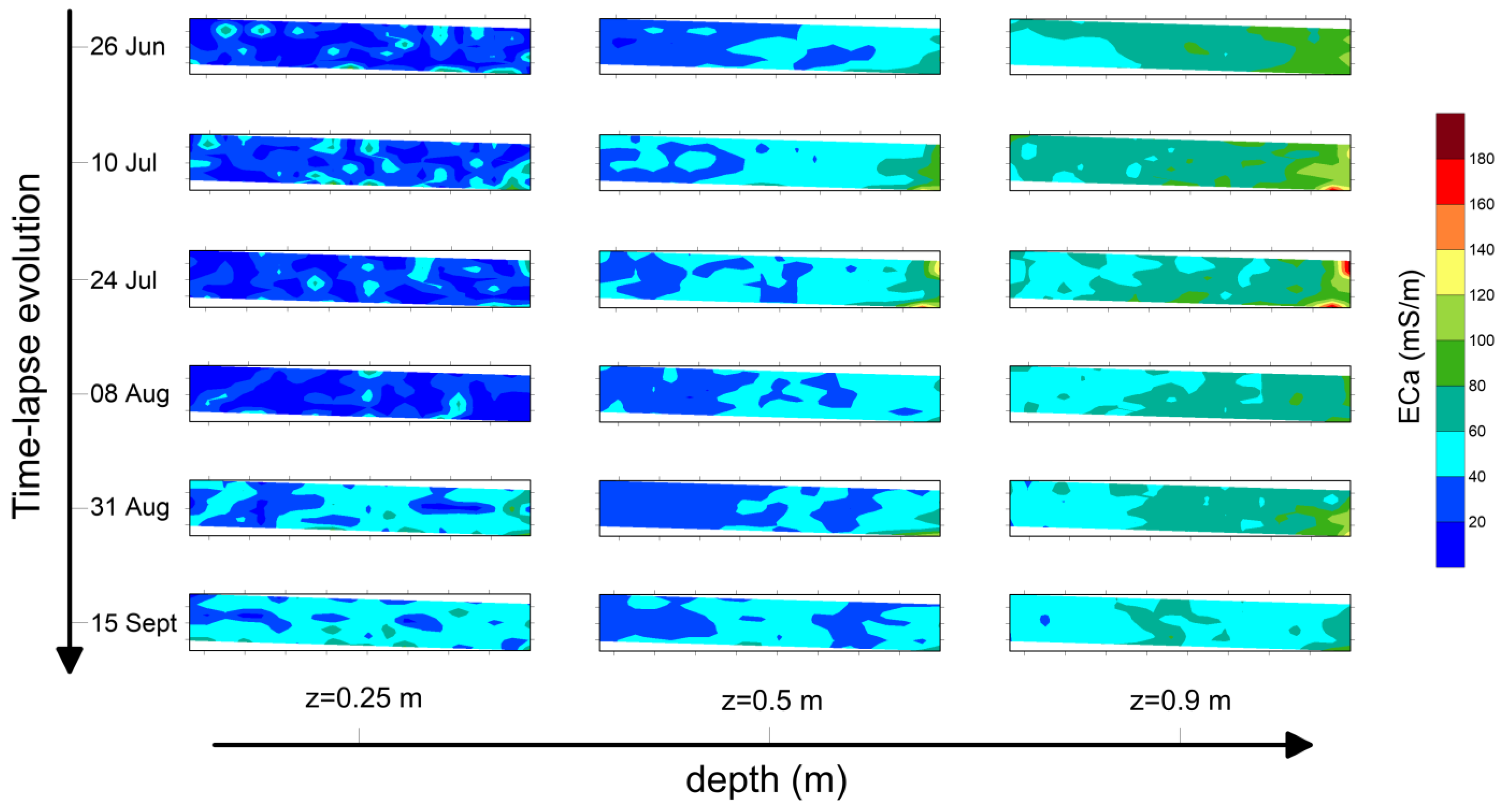
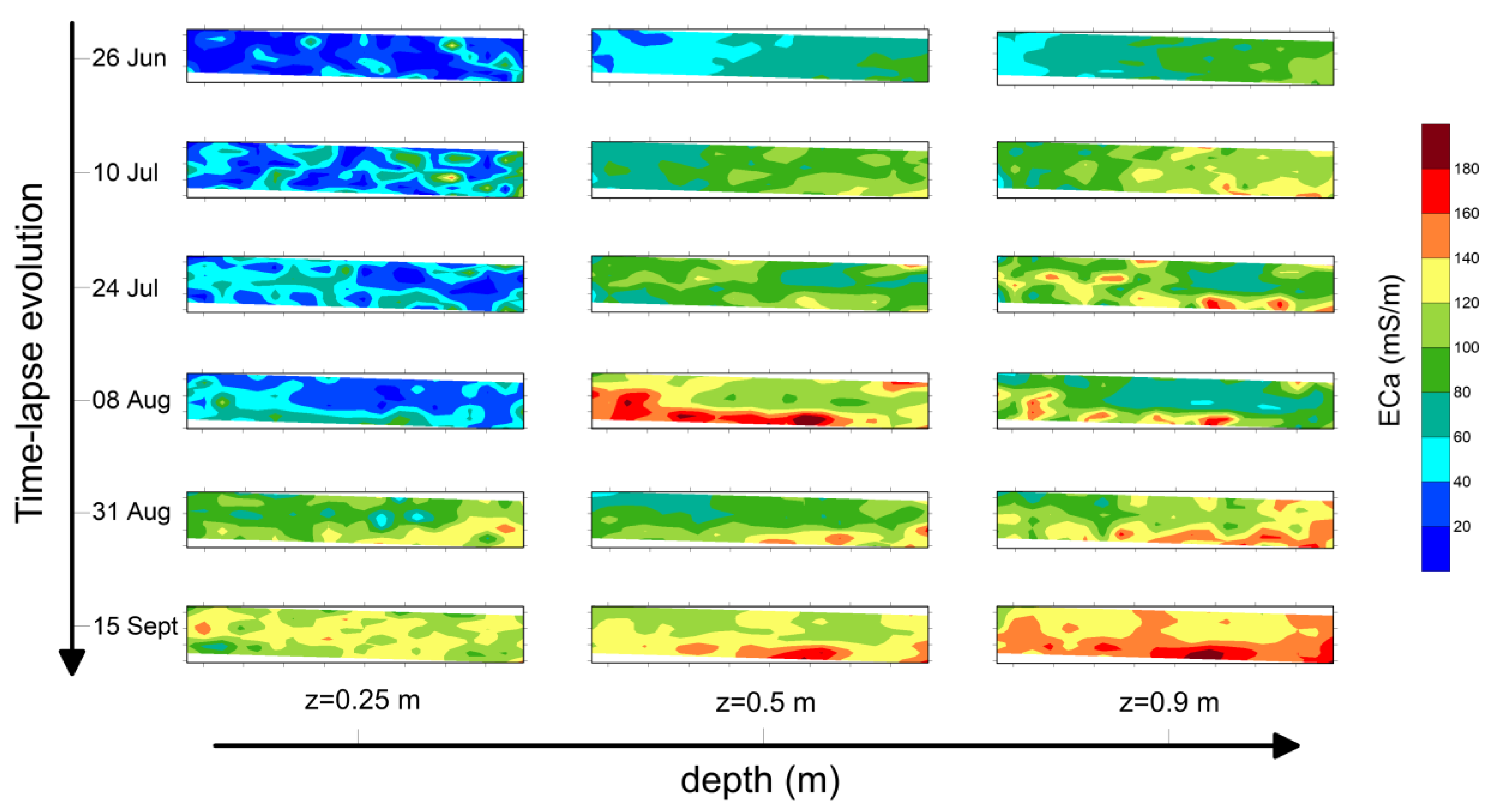
Figure 5 refers to maps produced for plot A2. Three different depths of investigation (z = 0.25 m, z = 0.5 m and z = 0.9 m, respectively) and six time instants have been considered.

Background conductivity, i.e., the map produced on 26 June, refers to ECa distribution before the start of irrigation. At z = 0.25 m, the ECa values range from 10 mS/m to 40 mS/m, while deeper soil layers (z = 0.5 m and z = 0.9 m) show ECa values of about 60–80 mS/m.

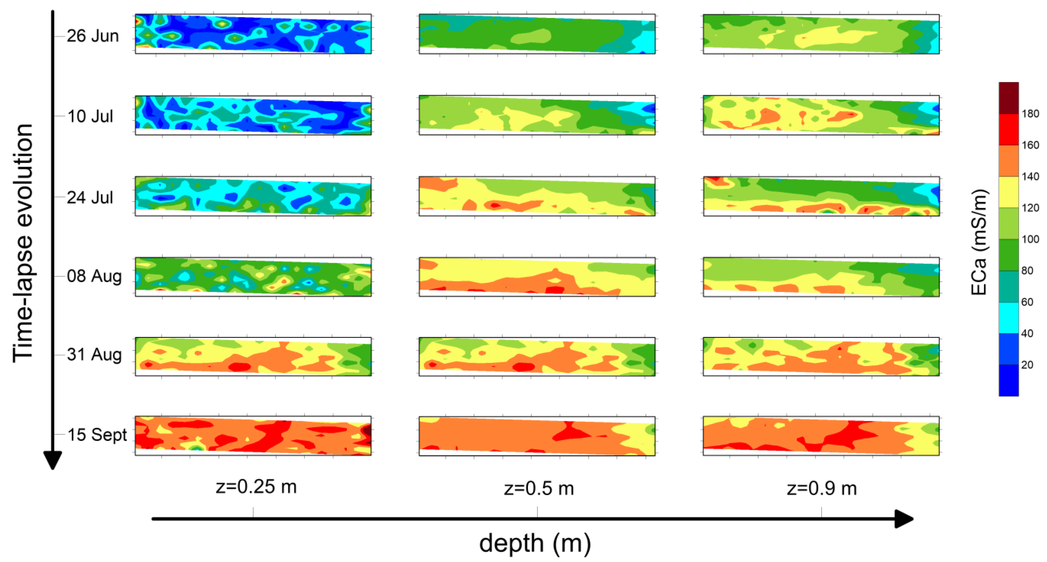
Figure 6 refers to the maps produced for plot B2 at the three selected depths. As for plot A2, background conductivity highlights a narrow range for z = 0.25 m (ECa ≈ 40 mS/m). Higher values at deeper layers have been observed (ECa ≈ 100 mS/m and ECa ≈ 120 mS/m for z = 0.5 m and z = 0.9 m, respectively).

Figure 7 shows maps obtained from plot C1. The trend is similar to that observed in B2, although a less marked increase in ECa is shown over time.

In fact, background conductivity observed at the three depths is comparable with those recorded in the other two plots, while time-lapse evolution highlights maximum values of ECa of 140 mS/m at z = 0.25 m and 160 mS/m at z = 0.5 m and z = 0.9 m.

Some local anomalous response causes small drifts from this general trend.

Figure 8 showed the average value of ECa calculated for the three plots at the six time points and plotted over time. In plot A2, ECa distribution is roughly steady over time, with values lower at the upper layer (z = 0.25 m) and higher in deeper ones (z = 0.5 m and z = 0.9 m). In plots B2 and C1, the increasing trend of ECa has been observed at all depths and is more marked in the upper layer (z = 0.25 m).

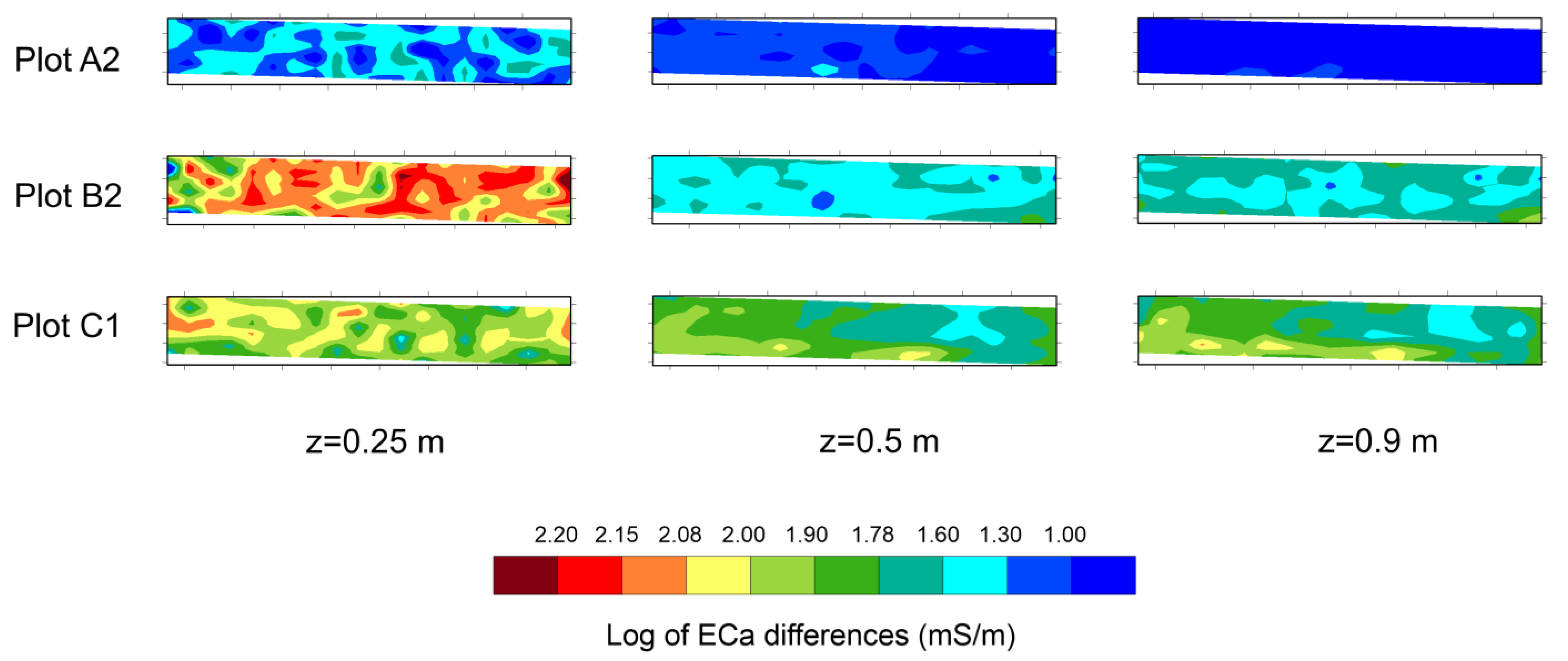
Finally, the differences between ECa values recorded in the last EMI dataset (15 September) and the first one (26 June) has been computed and visualized by the maps shown in Figure 9. At z = 0.25 m, higher contrast in ECa values has been recorded in plot B2, while lower changes have been observed in plot A2. In deeper layers (z = 0.5 m and z = 0.9 m), the changes are less clear and almost negligible in plot A2.

3.2. Soil Sampling Analysis

Table 6. Level of Na, Cl, pH and ECe of soil samples collected at two depths 0–0.2, 0.2–0.4. Each value is an average of 3 samples. Letters indicate statistically significant differences at p < 0.05 level of significance. n.s. indicates not significant.

Samples	Cl− (mg/L)	Na (mg/L)	pH	ECe (mS/cm)
A20	26.08 ± 3.52 n.s.	0.10 ± 0.01 n.s.	8.02 ± 0.21 n.s.	0.93 ± 0.01 b
B20	35.01 ± 9.23 n.s.	0.14 ± 0.03 n.s.	7.74 ± 0.13 n.s.	1.77 ± 0.15 a
C20	33.07 ± 6.23 n.s.	0.13 ± 0.02 n.s.	7.57 ± 0.09 n.s.	1.66 ± 0.17 a
A40	68.64 ± 1.9 a	0.14 ± 0.03 n.s	7.64 ± 0.28 n.s.	0.99 ± 0.07 b
B40	96.24 ± 5.38 b	0.13 ± 0.02 n.s	8.06 ± 0.03 n.s.	1.99 ± 0.28 a
C40	100.1 ± 6.22 b	0.15 ± 0.01 n.s	7.96 ± 0.06 n.s.	2.18 ± 0.29 a

shows the level of Na, Cl⁻, pH and ECe of soil samples at the end of irrigation season at two depths 0–0.20 m and 0.20–0.40 m. A high increase in ECe with respect to the initial value equal to 0.63 mS/cm has been observed in plots irrigated with AIW (plots B and C). Moreover, we observed a significant difference among treatments by comparing plots B and C irrigated with AIW with respect to plot A irrigated with FW. Soil pH and Cl⁻ levels did not change significantly for all treatments considered at a depth of 0–0.20 m. A significant increase in Cl⁻ soil concentration was observed in plot B irrigated with AIW at a dept of 0.20–0.40 m. Finally, at 0.20–0.40 m depth, we observed a significant increase in Na in plots B and C.

3.3. Correlation between Apparent Electrical Conductivity and Soil Electrical Conductivity

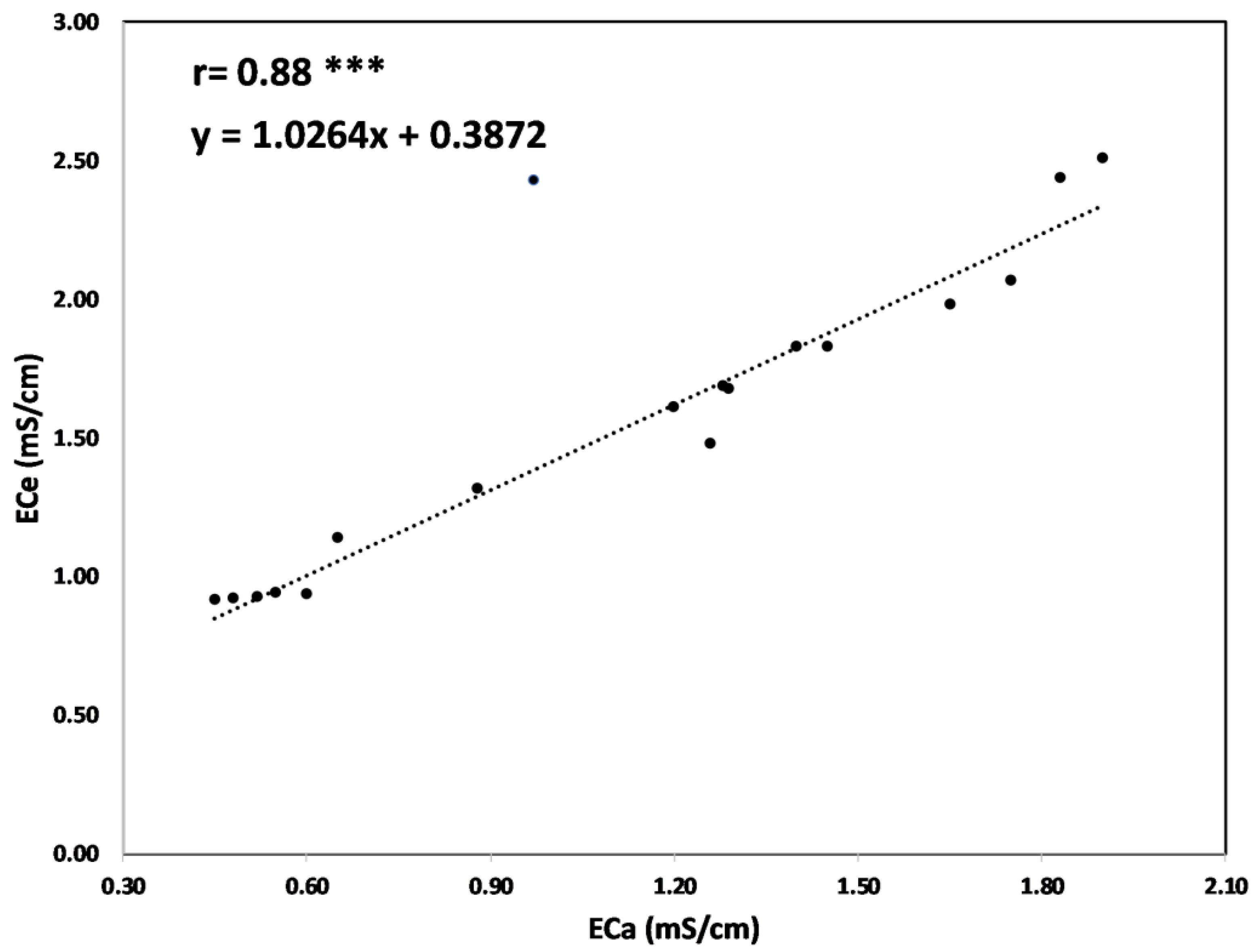
In order to derive a site-specific correlation function, 18 ECe values, obtained from nine sampling points at two different depths (0.20 m and 0.40 m), have been plotted with corresponding ECa values recorded in the same points (Figure 10). ECa values were converted from mS/m to mS/cm in order to be correctly correlated with Ece values measured on soil samples. The graph of Figure 8 highlights a clear exponential trend; as soil EC increases, ECa increases. Only one point shows an unexplained huge drift from this trend, probably due to a typing error in soil sampling data. This unexpected value was not considered for the formulation of the correlation function and for estimating the “r” Pearson’s correlation coefficient and the P-value. The correlation function covers a wide range of soil electrical conductivity (from 1 mS/cm to 2.5 mS/cm), suggesting that it can be assumed to be quite reliable.

4. Discussion

In terms of chemical parameters considered (Table 6), evident effects were found after 1 year of irrigation with AIW as compared to FW. ECe values (0.63 ± 0.12 mS/cm) at the beginning of the experiment were low in each plot and were consistent with values detected in other studies developed in the Apulian region [32]. At the end of the irrigation season, we observed an increase in ECe in plots irrigated with AIW (plots B and C). The significant increase in ECe was due to the higher concentrations of salt in waters (which reached the highest value of 4.45 mS/cm), as already observed by several authors [33,34,35]. Furthermore, the excess of nutrients used in plot B did not increase excessively the level of ECe. In fact, as reported by [36], the application of fertilizers by using irrigation water (fertigation) can reduce soil salinization and mitigate salt stress effects because it improves the efficiency of fertilizer use. Moreover, even though high concentrations of sodium could increase pH (alkalinization) [36], in our case a high level of potassium in AIW may have mitigated the negative effect of high levels of sodium. Chlorine concentration was significantly higher in plots irrigated with Agro-industrial wastewater (AIW) + conventional fertigation (plots B) and in plot C probably due to the high levels of this anion in water and the excessive use of fertilizers during the irrigation season.

The soil sampling points were essential for establishing an accurate calibration relationship between ECa and ECe to convert the geophysical parameter into an agronomic one.

Geophysical analysis has revealed some key points of geophysical prospecting, both for static imaging before the irrigation test and for spatio-temporal dynamics of ECa during the irrigation season. In fact, the narrow range shown at z = 0.25 m in background ECa distribution (26 June) of the three plots highlights a quite homogeneous electrical behavior of the soil, denoting no significant variations in terms of soil textural properties. As the depth increases (z = 0.5 m and z = 0.9 m), ECa values increase probably due to a soil textural change, different compaction degree, soil moisture or a mixture of them.

As expected, the response of soils irrigated with saline reclaimed water is quite different compared with plots irrigated with freshwater. In fact, a significant increase in ECa over time has been observed in the former, while negligible variations have been recorded in the latter. The time-lapse maps observed at z = 0.25 m for plot A2 (Figure 5) show negligible changes in ECa distribution until 8 August; then, a slight increase was recorded until the end of monitoring (ECa ≈ 60 mS/m at 15 September), while no significant changes are visualized at z = 0.5 m and z = 0.9 m. Indeed, a slight decrease is observed at z = 0.9 m.

On the contrary, significant changes in ECa distribution can be observed in the time-lapse evolution for both plots B2 and C1, as clearly visualized by color changing observed in the maps. In terms of salinity trends derived from ECa, two main aspects can be inferred. First, salt accumulation was enhanced in the upper soil layer, within 0.25 m from ground surface, but it was not negligible in the deeper layer, which is up to 1 m from the ground surface. Moreover, this trend is mainly observed from the second part of the irrigation season. This is consistent with the observed scientific evidence concerning soil–plant–water interaction when saline water is used for irrigation. In fact, high osmotic pressure that inhibits water flow from the soil to the plant causes slow salt accumulation over time into soil by inducing its higher increase in the second part of the season.

The different impacts of irrigation water quality on ECa distribution were highlighted in the Figure 9 and Figure 10. In particular, the comparison among three graphs clearly highlights how treated wastewater affects ECa distribution during the irrigation season. On the other hand, Plot A2 shows no significant changes except for a slight increase in the upper soil layer, and Plot B2 and Plot C1 highlight a remarkable raise of ECa, which is much more marked in the top layer than in depth. The ECa increase seems to be more enhanced in the second part of irrigation season, i.e., since the beginning of August, with respect to the first one.

5. Conclusions

The use of reclaimed water as irrigation source can represent an efficient strategy in agriculture to reduce anthropogenic pressure on freshwater, to limit the use of synthetic chemical fertilizers and to produce benefit to crops by providing organic matter and nutrients. At the same time, serious degradation of soil quality could be induced by salt and heavy metals accumulation due to the quality of applied irrigation water that can significantly change soil salinity.

For this purpose, in order to avoid salts and/or toxic substances accumulation, real time mapping of soil properties is needed, which requires rapid, noninvasive and reliable measurement techniques. This is a crucial issue considering the increased demand for quantitative high-resolution soil maps.

This study proposes electromagnetic induction measurements to evaluate the impact on soil properties of saline-reclaimed water used for irrigation. Electromagnetic data collected several times during irrigation season allowed monitoring the time-lapse evolution of the ECa parameter.

This study showed that the noncontacting electromagnetic approach was proved to be an effective tool for mapping ECa, used as a proxy for soil salinity, by providing an added value to soil investigation for agriculture purposes.

In fact, compared with point scale direct sampling, EMI data allowed mapping a large area in short period of time with an unprecedented level of detail.

The results suggest that the integrated agro-geophysical approach can be used as an effective supporting tool for large-scale monitoring of soil salinity; the capability to update soil salinity maps in real time can allow estimating the amount of accumulated salts in medium to long-term periods and preventing soil salinization risks over time.

References

- Vivaldi, G.A.; Camposeo, S.; Lopriore, G.; Romero-Trigueros, C.; Pedrero, F. Using saline reclaimed water on almond grown in Mediterranean conditions: Deficit irrigation strategies and salinity effects. Water Supply 2019, 19, 1413–1421. [Google Scholar] [CrossRef]
- Pedrero, F.; Alarcón, J.J.; Nicolás, E.; Mounzer, O. Influence of irrigation with saline reclaimed water on young grapefruits. Desalin. Water Treat. 2013, 51, 2488–2496. [Google Scholar] [CrossRef]
- Doolittle, J.A.; Brevik, E.C. The use of electromagnetic induction techniques in soils studies. Geoderma 2014, 223–225, 33–45. [Google Scholar] [CrossRef] [Green Version]
- Allred, B.J.; Daniels, J.J.; Ehsani, M.R. Handbook of Agricultural Geophysics, 1st ed.; CRC Press, Taylor & Francis Group: Boca Raton, FL, USA, 2008; 432p. [Google Scholar]
- Shirzaditabar, F.; Heck, R.J. Characterization of soil drainage using electromagnetic induction measurement of soil magnetic susceptibility. Catena 2021, 207, 105671. [Google Scholar] [CrossRef]
- Koganti, T.; Van De Vijver, E.; Allred, B.J.; Greve, M.H.; Ringgaard, J.; Iversen, B.V. Mapping of Agricultural Subsurface Drainage Systems Using a Frequency-Domain Ground Penetrating Radar and Evaluating Its Performance Using a Single-Frequency Multi-Receiver Electromagnetic Induction Instrument. Sensors 2020, 20, 3922. [Google Scholar] [CrossRef]
- Romero-Ruiz, A.; Linde, N.; Keller, T.; Or, D. A review of geophysical methods for soil structure characterization. REV Geophys. 2019, 56, 672–697. [Google Scholar] [CrossRef] [Green Version]
- Altdorff, D.; Bechtold, M.; van der Kruk, J.; Vereecken, H.; Huisman, J.A. Mapping peat layer properties with multicoil offset electromagnetic induction and laser scanning elevation data. Geoderma 2016, 261, 178–189. [Google Scholar] [CrossRef]
- Cheng, Q.; Tao, M.; Chen, X.; Binley, A. Evaluation of electrical resistivity tomography (ERT) for mapping the soil–rock interface in karstic environments. Environ. Earth Sci. 2019, 78, 1–14. [Google Scholar] [CrossRef] [Green Version]
- Martini, E.; Werban, U.; Zacharias, S.; Pohle, M.; Dietrich, P.; Wollschläge, U. Repeated electromagnetic induction measurements for mapping soil moisture at the field scale: Validation with data from a wireless soil moisture monitoring network. Hydrol. Earth Syst. Sci. 2017, 21, 495–513. [Google Scholar] [CrossRef] [Green Version]
- Calamita, G.; Perrone, A.; Brocca, L.; Onorati, B.; Manfreda, S. Field test of a multi-frequency electromagnetic induction sensor for soil moisture monitoring in southern Italy test sites. J. Hydrol. 2015, 529, 316–329. [Google Scholar] [CrossRef]
- Cimpoiaşu, M.O.; Kuras, O.; Pridmore, T.; Mooney, S.J. Potential of geoelectrical methods to monitor root zone processes and structure: A review. Geoderma 2020, 365, 114232. [Google Scholar] [CrossRef]
- De Carlo, L.; Battilani, A.; Solimando, D.; Caputo, M.C. Application of time-lapse ERT to determine the impact of using brackish wastewater for maize irrigation. J. Hydrol. 2020, 582, 124465. [Google Scholar] [CrossRef]
- Mary, B.; Peruzzo, L.; Boaga, J.; Cenni, N.; Schmutz, M.; Wu, Y.; Hubbard, S.S.; Cassiani, G. Time-lapse monitoring of root water uptake using electrical resistivity tomography and mise-à-la-masse: A vineyard infiltration experiment. Soil 2020, 6, 95–114. [Google Scholar] [CrossRef] [Green Version]
- Vanella, D.; Cassiani, G.; Busato, L.; Boaga, J.; Barbagallo, A.; Binley, A.; Consoli, S. Use of small scale electrical resistivity tomography to identify soil-root interactions during deficit irrigation. J. Hydrol. 2018, 556, 310–324. [Google Scholar] [CrossRef] [Green Version]
- Shanahan, P.W.; Binley, A.; Whalley, R.W.; Watts, C.W. The Use of Electromagnetic Induction to Monitor Changes in Soil Moisture Profiles beneath Different Wheat Genotypes. Soil Sci. Soc. Am. J. 2015, 79, 459–466. [Google Scholar] [CrossRef] [Green Version]
- Rossi, R.; Amato, M.; Bitella, G.; Bochicchio, R.; Ferreira Gomes, J.J.; Lovelli, S.; Martorella, E.; Favale, P. Electrical resistivity tomography as a non-destructive method for mapping root biomass in an orchard. Eur. J. Soil Sci. 2011, 62, 206–215. [Google Scholar] [CrossRef]
- Amato, M.; Basso, B.; Celano, G.; Bitella, G.; Morelli, G.; Rossi, R. In situ detection of tree root distribution and biomass by multi-electrode resistivity imaging. Tree Physiol. 2008, 28, 1441–1448. [Google Scholar] [CrossRef] [PubMed]
- Blanchy, G.; Watts, C.W.; Ashton, R.W.; Webster, C.P.; Hawkesford, M.J.; Whalley, W.R.; Binley, A. Accounting for heterogeneity in the θ–σ relationship: Application to wheat phenotyping using EMI. Vadose Zone J. 2020, 19, e20037. [Google Scholar] [CrossRef]
- Paz, M.C.; Farzamian, M.; Paz, A.M.; Castanheira, N.L.; Gonçalves, M.C.; Monteiro Santos, F. Assessing soil salinity dynamics using time-lapse electromagnetic conductivity imaging. Soil 2020, 6, 499–511. [Google Scholar] [CrossRef]
- Scudiero, E.; Skaggs, T.H.; Corwin, D.L. Simplifying field-scale assessment of spatiotemporal changes of soil salinity. Sci. Total Environ. 2017, 587–588, 273–281. [Google Scholar] [CrossRef] [PubMed]
- Yao, R.; Yang, J.; Wu, D.; Xie, W.; Gao, P.; Jin, W. Digital Mapping of Soil Salinity and Crop Yield across a Coastal Agricultural Landscape Using Repeated Electromagnetic Induction (EMI) Surveys. PLoS ONE 2016, 11, e0153377. [Google Scholar] [CrossRef] [PubMed]
- Corwin, D.L.; Lesch, S.M. Protocols and guidelines for field-scale measurement of soil salinity distribution with ECa-directed soil sampling. J. Environ. Eng. Geophys. 2013, 18, 1–25. [Google Scholar] [CrossRef] [Green Version]
- Farzamian, M.; Autovino, D.; Basile, A.; De Mascellis, R.; Dragonetti, G.; Monteiro Santos, F.; Binley, A.; Coppola, A. Assessing the dynamics of soil salinity with time-lapse inversion of electromagnetic data guided by hydrological modelling. Hydrol. Earth Syst. Sci. 2021, 25, 1509–1527. [Google Scholar] [CrossRef]
- Moghadas, D.; Jadoon, K.Z.; McCabe, M.F. Spatiotemporal monitoring of soil water content profiles in an irrigated field using probabilistic inversion of time-lapse EMI data. Adv. Water Resour. 2017, 110, 238–248. [Google Scholar] [CrossRef] [Green Version]
- Jadoon, K.Z.; Moghadas, D.; Jadoon, A.; Missimer, T.M.; Al-Mashharawi, S.K.; McCabe, M.F. Estimation of soil salinity in a drip irrigation system by using joint inversion of multicoil electromagnetic induction measurements. Water Resour. Res. 2015, 51, 3490–3504. [Google Scholar] [CrossRef] [Green Version]
- Von Hebel, C.; Rudolph, S.; Mester, A.; Huisman, J.A.; Kumbhar, P.; Vereecken, H.; van der Kruk, J. Three-dimensional imaging of subsurface structural patterns using quantitative large-scale multiconfiguration electromagnetic induction data. Water Resour. Res. 2014, 50, 2732–2748. [Google Scholar] [CrossRef] [Green Version]
- Monteiro Santos, F.A. 1-D laterally constrained inversion of EM34 profiling data. J. Appl. Geophys. 2004, 56, 123–134. [Google Scholar] [CrossRef]
- McNeill, J.D. Electromagnetic Terrain Conductivity Measurement at Low Induction Numbers; Geonics Limited: Mississauga, ON, Canada, 1980; Available online: http://www.geonics.com/pdfs/technicalnotes/tn6.pdf (accessed on 19 July 2018).
- Callegary, J.B.; Ferré, T.P.A.; Groom, R.W. Vertical spatial sensitivity and exploration depth of low-induction-number electromagnetic-induction instruments. Vadose Zone J. 2007, 6, 158–167. [Google Scholar] [CrossRef]
- Richards, L.A. Diagnosis and Improvement of Saline Alkali Soils; Handbook n.60; U.S. Department of Agriculture (USDA): Washington, DC, USA, 1954; 160p. [Google Scholar]
- Ancona, V.; Bruno, D.E.; Lopez, N.; Pappagallo, G.; Uricchio, V.F. A modified soil quality index to assess the influence of soil degradation processes on desertification risk: The Apulia case. Ital. J. Agron. 2010, 3, 45–55. [Google Scholar] [CrossRef] [Green Version]
- Libutti, A.; Gatta, G.; Gagliardi, A.; Vergine, P.; Pollice, A.; Beneduce, L.; Disciglio, G.; Tarantino, E. Agro-industrial wastewater reuse for irrigation of a vegetable crop succession under Mediterranean conditions. Agric. Water Manag. 2017, 196, 1–14. [Google Scholar] [CrossRef]
- Vergine, P.; Salerno, C.; Libutti, A.; Beneduce, L.; Gatta, G.; Berardi, G.; Pollice, A. Closing the water cycle in the agro-industrial sector by reusing treated wastewater for irrigation. J. Clean. Prod. 2017, 164, 587–596. [Google Scholar] [CrossRef]
- Disciglio, G.; Gatta, G.; Libutti, A.; Gagliardi, A.; Carlucci, A.; Lops, F.; Cibelli, F.; Tarantino, A. Effects of irrigation with treated agro-industrial wastewater on soil chemical characteristics and fungal populations during processing tomato crop cycle. J. Soil Sci. Plant Nutr. 2015, 15, 765–780. [Google Scholar] [CrossRef] [Green Version]
- Machado Almeida, R.M.; Serralheiro, R.P. Soil salinity: Effect on vegetable crop growth. Management practices to prevent and mitigate soil salinization. Horticulturae 2017, 3, 30. [Google Scholar] [CrossRef]
Figure 1.
Satellite map of the study area (Google Earth image): (a) experimental field belonging to the Fiordelisi farm; (b) details of the experimental area with irrigation setup.
Figure 2.
Basics of electromagnetic induction technique.
Figure 3.
Cumulative sensitivity (CS) for three Mini-Explorer sensors: (a) VCP configuration and (b) HCP configuration coil.
Figure 4.
(a) Distribution of EMI point measurement location in the experimental area and (b) partitioning of the experimental area in nine plots with different irrigation setup.
Figure 5.
Maps of ECa recorded on the plot A2 for 3 depths (z = 0.25 m, z = 0.5 m and z = 0.9 m) and 6 temporal steps.
Figure 6.
Maps of ECa recorded on the plot B2 for three depths (z = 0.25 m, z = 0.5 m and z = 0.9 m) and six temporal steps.
Figure 7.
Maps of ECa recorded on the plot C1 for three depths (z = 0.25 m, z = 0.5 m and z = 0.9 m) and six temporal steps.
Figure 8.
Average ECa value recorded in each plot over time at three different depths.
Figure 9.
Differences in ECa values computed by comparing the last EMI dataset (15 September) and the first one (26 June).
Figure 10.
ECe vs. ECa correlation function. The number of points of the fitting curve is 18. Statistically significant at p-value significance level: * 0.05, ** 0.01, *** 0.001 levels of significance.