Article

Projected Changes in Terrestrial Vegetation and Carbon Fluxes under 1.5 °C and 2.0 °C Global Warming

1
Key Laboratory of Meteorological Disaster, Ministry of Education/International Joint Research Laboratory of Climate and Environment Change (ILCEC)/Collaborative Innovation Center on Forecast and Evaluation of Meteorological Disasters, Nanjing University of Information Science and Technology, Nanjing 210044, China
2
School of Atmospheric Sciences, Nanjing University of Information Science and Technology, Nanjing 210044, China
*
Author to whom correspondence should be addressed.
Atmosphere 2022, 13(1), 42; https://doi.org/10.3390/atmos13010042
Submission received: 1 November 2021 / Revised: 14 December 2021 / Accepted: 26 December 2021 / Published: 28 December 2021

Abstract

:
The terrestrial ecosystem plays a vital role in regulating the exchange of carbon between land and atmosphere. This study investigates how terrestrial vegetation coverage and carbon fluxes change in a world stabilizing at 1.5 °C and 2 °C warmer than pre-industrial level. Model results derived from 20 Earth System Models (ESMs) under low, middle, and high greenhouse emission scenarios from CMIP5 and CMIP6 are employed to supply the projected results. Although the ESMs show a large spread of uncertainties, the ensemble means of global LAI are projected to increase by 0.04 ± 0.02 and 0.08 ± 0.04 in the 1.5 and 2.0 °C warming worlds, respectively. Vegetation density is projected to decrease only in the Brazilian Highlands due to the decrease of precipitation there. The high latitudes in Eurasia are projected to have stronger increase of LAI in the 2.0 °C warming world compared to that in 1.5 °C warming level caused by the increase of tree coverage. The largest zonal LAI is projected around 70° N while the largest zonal NPP is projected around 60° N and equator. The zonally inhomogeneous increase of vegetation density and productivity relates to the zonally inhomogeneous increase of temperature, which in turn could amplify the latitudinal gradient of temperature with additional warming. Most of the ESMs show uniform increases of global averaged NPP by 10.68 ± 8.60 and 15.42 ± 10.90 PgC year−1 under 1.5 °C and 2.0 °C warming levels, respectively, except in some sparse vegetation areas. The ensemble averaged NEE is projected to increase by 3.80 ± 7.72 and 4.83 ± 10.13 PgC year−1 in the two warming worlds. The terrestrial ecosystem over most of the world could be a stronger carbon sink than at present. However, some dry areas in Amazon and Central Africa may convert to carbon sources in a world with additional 0.5 °C warming. The start of the growing season in the northern high latitudes is projected to advance by less than one month earlier. Five out of 10 CMIP6 ESMs, which use the Land Use Harmonization Project (LUH2) dataset or a prescribed potential vegetation distribution to constrain the future change of vegetation types, do not reduce the model uncertainties in projected LAI and terrestrial carbon fluxes. This may suggest the challenge in optimizing the carbon fluxes modeling in the future.

1. Introduction

Atmospheric CO2 concentration has nearly doubled since the industrial revolution due to fossil fuel combustion and other human activities, which is believed to be an important reason leading to the significant increase of global average temperature [1,2,3]. Terrestrial ecosystem productivity from global to regional scales is altered by the availabilities of heat, water, solar radiation, and nutrients [4,5,6,7,8]. Spatial and temporal variabilities of precipitation are changing in response to the global warming [9,10]. Extreme flooding and drought events are reported to occur more frequently, incurring a higher level of climate risks than the pre-industrial period to the human dependent ecosystem and environment [11]. To alleviate the risks posed by climate change, the Paris Agreement committed to pursue the goal of staying below 2.0 °C above pre-industrial levels, preferably pursuing efforts to limit temperature increase to 1.5 °C [12].
The latest studies have investigated the possible future responses in atmospheric circulation, freshwater system, biomass energy, etc., to the 1.5 and 2.0 °C warmings [13,14,15]. It is pointed out that a stabilizing temperature at 1.5 °C warming probably will reduce global mean sea-level (GMSL) and mitigate the effects of rising GMSL relative to the 2.0 °C scenario [16,17]. Aerenson et al. [18] found that precipitation and temperature extremes change significantly in high latitudes with 1.5 and 2.0 °C warming. Kong et al. [19] indicated that permafrost degradation in the Northern Hemisphere is projected to occur mainly in the southern Central Siberian Plateau when global warming reaches 1.5 °C. Most of recent research agrees that 0.5 °C additional warming would lead to more frequent and intense changes of the climate system. To understand how the climate system would change under specified warming scenarios is extremely valuable and a challenge for policy makers and researchers.
Among the climate system, the terrestrial ecosystem is an important element of the global carbon cycle as it is a major sink and source of atmospheric CO2 through the biogeophysical and biogeochemical processes. Vegetation distribution and density are substantially influenced by local climate, and meantime it plays an important role in affecting climate through its impact on exchanges of carbon, water, energy and momentum between land and atmosphere [20]. The global warming-induced change of terrestrial carbon of sinks and sources vary over space and time [21]. The global warming is expected to have a diverse impact on vegetation [22]. In most cases, an increase in temperature is beneficial to vegetation by enhancing metabolism and extending the growing season. However, higher than the optimum temperature probably produces negative impacts on the photosynthesis, growth, productivity, and water use efficiency of vegetation [23,24,25]. For example, Mao et al. [26] found that climate warming could explain a significant increase in annual vegetation growth from 1982–2009, whereas higher levels of warming in some areas may produce adverse results by changing the stomatal conductance of leaves [27]. Yue et al. [28] found that the corresponding reduction in CO2 and pollution emissions will bring more benefits to the ecosystem in China compared with the pathway without emission control in a world of 1.5 °C warming.
However, quantification of carbon pools and fluxes is complex and carries large uncertainties [29]. For instance, Friedlingstein et al. [30] considered the uncertainty in CO2 projections was mainly attributable to uncertainties in the response of the land carbon cycle. Huntzinger et al. [31] found that the most recently used land models are inconsistent in the primary driver of cumulative carbon uptake for 85% of vegetated land area. The representation of vegetation dynamics in different land models could introduce additional uncertainties for the future projection of terrestrial carbon fluxes [32]. Therefore, it is more reliable using the ensemble of model results to supply the future changes of variables with the model extensions.
Recently, more models participating the Coupled Model Intercomparison Project Phase, Phase 6 (CMIP6) have been making their results available by courtesy of scientists’ worldwide endeavors. The CMIP6 models are shown to have better performance in simulating climate changes to some degree due to the improved model schemes and refined resolution [33,34,35]. More CMIP6 than CMIP5 models incorporate the terrestrial ecosystem or global dynamic vegetation component, supplying us more members of model projections in exploring the possible future change of terrestrial vegetation and carbon fluxes. Note that some of CMIP6 ESMs use the vegetation functional type map from the dataset of Land Use Harmonization Project (LUH2 [36]) or a prescribed potential vegetation distribution to provide the future vegetation coverages, which may supply more informative and consistent results.
In this study, we employed the ESM’ outcome from both CMIP5 and CMIP6 to explore the future change of leaf area index (LAI), the vegetation coverage, as well as some primary variables of terrestrial carbon fluxes. We aim at providing more qualitative and quantitative information of the possible future changes in terrestrial ecosystem and carbon cycle when 1.5 °C and 2.0 °C warming levels are reached. Beyond that, we compare the simulation results of CMIP6 ESMs to the CMIP5 models and try to investigate the differences of the two groups of models in supplying the projected terrestrial vegetation and carbon fluxes.

2. Data and Methods

2.1. CMIP5 and CMIP6 Data

To investigate the future changes of terrestrial vegetation and carbon fluxes, as well as the related environmental conditions, monthly output simulated by Earth System Models (ESMs) participating in the Coupled Model Intercomparison Project Phase 5 and Phase 6 (CMIP5 and CMIP6. https://esgf-node.llnl.gov/, accessed on 10 December 2021) are used in this study. Ten ESMs from CMIP5 (Table 1) and 10 ESMs from CMIP6 (Table 2) considering the synchronized response of terrestrial productivity to climate have been selected in this study. The selected CMIP5 ESMs use global dynamic vegetation model to simulate vegetation composition and distributions. But the selected CMIP6 ESMs use two kinds of approach to hand the future change of vegetation types. One applies the synchronically simulated vegetation types using the dynamic vegetation models as those in CMIP5 ESMs, such as the BCC-CSM2-MR, CanESM5, GFDL-ESM4, and the EC-Earth3 (EC-Earth3-CC, EC-Earth3-Veg) family ESMs. The other is using the vegetation functional type map from the dataset of Land Use Harmonization Project (LUH2 [36]), such as the IPSL-CM6A-LR, MPI-ESM1-2-LR, and CESM2, or a prescribed potential vegetation distribution such as the INM (INM-CM4-8, INM-CM5-0) family model. The vegetation functional types supplied by LUH2 smoothly connect historical reconstructions of land use with future projections.
The variables analyzed here are 2-m air temperature (TAS), precipitation (PR), near-surface relative humidity (RH), 10-m wind speed (Wind), leaf area index (LAI), net primary production (NPP) and heterotrophic respiration (HR). The net ecosystem exchange (NEE) is calculated by NPP minus HR. Model results are derived from historical simulations, and future simulations under representative concentration pathways (RCP2.6, RCP4.5 and RCP8.5) in CMIP5, and shared socioeconomic pathways (SSP126, SSP245 and SSP585) in CMIP6. The bilinear interpolation method is used to unify the spatial resolution of model results as 64 × 128.
The 20-year baseline in 1986–2005 is defined as the reference period in this study, when the temperature is 0.61 °C higher than the pre-industrial level [1]. Therefore, an increase of 0.89 °C and 1.39 °C above the baseline level is defined as 1.5 °C and 2.0 °C above the pre-industrial level respectively. The 20-year running average annual temperature is used to specify the 20-year period when 1.5 °C or 2.0 °C warming level is reached. We then obtained the 1.5 °C and 2.0 °C analysis period for each model under different scenarios based on respective historical simulation data (Figure 1). Basically, the warming thresholds are projected to reach earlier under RCP8.5/SSP585 than the others except MIROC-ESM-CHEM, EC-Earth3-CC and IPSL-CM6A-LR reaching the 1.5 °C warming level. And the ESMs agree more on the time period when 1.5 °C warming occurs than on the time period with 0.5 °C additional warming. 7/10 CMIP5 ESMs and 6/10 CMIP6 ESMs may not reach the 2.0 °C warming level under the low greenhouse emission scenario. Overall, the GFDL-ESM2G is projected to reach the specified warming levels the latest, while the CanESM5 and HadGEM2-ES are projected to reach these levels first.

2.2. Signal-to-Noise Ratio

The differences in the structure of the modules and their coupling methods are testified to cause the inconsistency in the simulation results of each model [1]. In order to show the solidity or specification of the change simulated by ESMs, we define the signal-to-noise ratio (S/N) as Equation (1) to judge the consistency of model results.
S / N = mean   absolute   value   of   future   change   ( S ) standard   deviation   ( N )
Here S is the absolute value of ensemble average of the simulated future changes; N is the mean value of the standard deviation between simulations. S/N > 1 represents that the simulation results pass the consistency test, and the ESMs agree on the sign of future change. The higher the value of the S/N, the better the consistency of the model simulation results.

3. Results

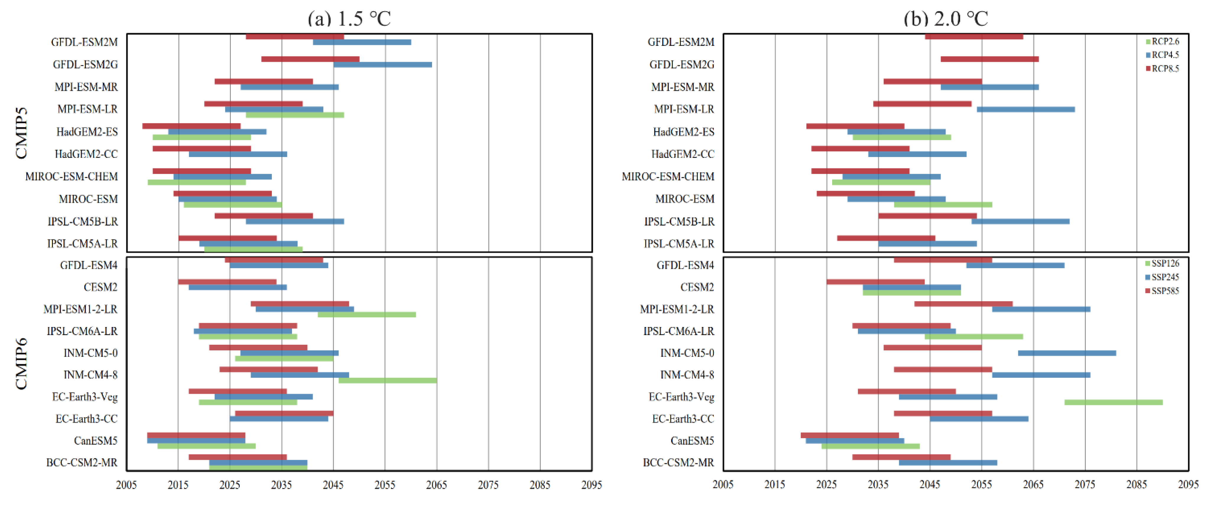
3.1. Future Changes of Climate

We first analyzed the projected future changes of 2-m air temperature, precipitation, near-surface relative humidity and 10-m wind speed with their inter-scenario and inter-model uncertainties when the warming levels of 1.5 °C and 2.0 °C were reached. Differences between these two warming levels were analyzed as well to explore the impact of the additional 0.5 °C warming compared to the 1.5 °C warming level.
Figure 2a–c show the spatially inhomogeneous increase of surface temperature with the large increases in the high latitudes of Northern Hemisphere and over the Tibetan Plateau. The largest increase of precipitation is projected in areas around 60° N, Sahel, and India Peninsula. The Amazon region and South Africa are projected to be drier in 1.5 °C warming world than present. The magnitude of drying could be double or even triple in the 2.0 °C warming world (Figure 2d–f). Generally, wind speed is projected to decrease in the Northern Hemisphere especially in the mid-high latitudes in a world with additional 0.5 °C warming, and increase the most in Brazilian Highland, in which area near-surface relative humidity decreases the most. The largest increase of near-surface relative humidity is in the northern edge of Sahel, which causes the zonal average around 13° N, the largest through all latitudes (Figure 2g–h). In general, the 20 ESMs under different GHG emission scenarios show good consistency on the zonal averages of PR, RH, and wind changes when temperature reaches certain levels.
The ensemble means of averaged 2-m temperature change over land is projected to be 1.27 °C and 1.97 °C, respectively, which are higher than the global mean levels of 0.89 °C and 1.39 °C. The increase of 2-m temperature is shown to be intensified latitude-band by latitude-band from the Southern to the Northern Hemisphere, especially under the warming of 2.0 °C. It suggests that the inhomogeneous spatial pattern of temperature increase and the land–sea difference of surface temperature would be intensified continuously. The largest increase of latitudinal averaged precipitation is shown in HigNH (60–90° N), while the largest decrease is in MidSH (30–60° S). Except for the LowNH (0–30° N), the averages of relative humidity changes in other latitude zones are projected to decrease. The average of 10-m wind speed in the Southern Hemisphere over land is projected to change little but generally decrease in different latitude zones in the Northern Hemisphere. Moreover, most ESMs agree that the near surface wind would reach the largest decrease in MidNH (30–60° N) (Figure 3).
Additionally, we selected six regions according to the distribution of LAI changes to study the monthly variations of climate changes from a regional perspective (Figure 4). The squares in Figure 5a show the selected areas in northeastern Asia (EA), eastern Europe (EU), Congo Basin, eastern US (EUSA), Amazon (Amzn1), and Brazilian Highland (Amzn2). The seasonality of surface temperature is projected to change little in EA and EU. But precipitation is projected to reach the peak one month later in June with additional 0.5 °C warming in EA. The spring-to-early-summer season is projected to be warmer, drier, and has more rainfall than the other seasons of the year in EA and EU. Among all the selected regions, the Brazilian Plateau is projected to have the largest decrease of precipitation and relative humidity. In Brazilian Highland, precipitation and near-surface relative humidity are projected to decrease throughout the year except for a slight increase in precipitation in December and January. Future 10-m wind speed in Congo and Amazon are projected to be essentially unchanged when global average temperature hits 1.5 °C and 2.0 °C.

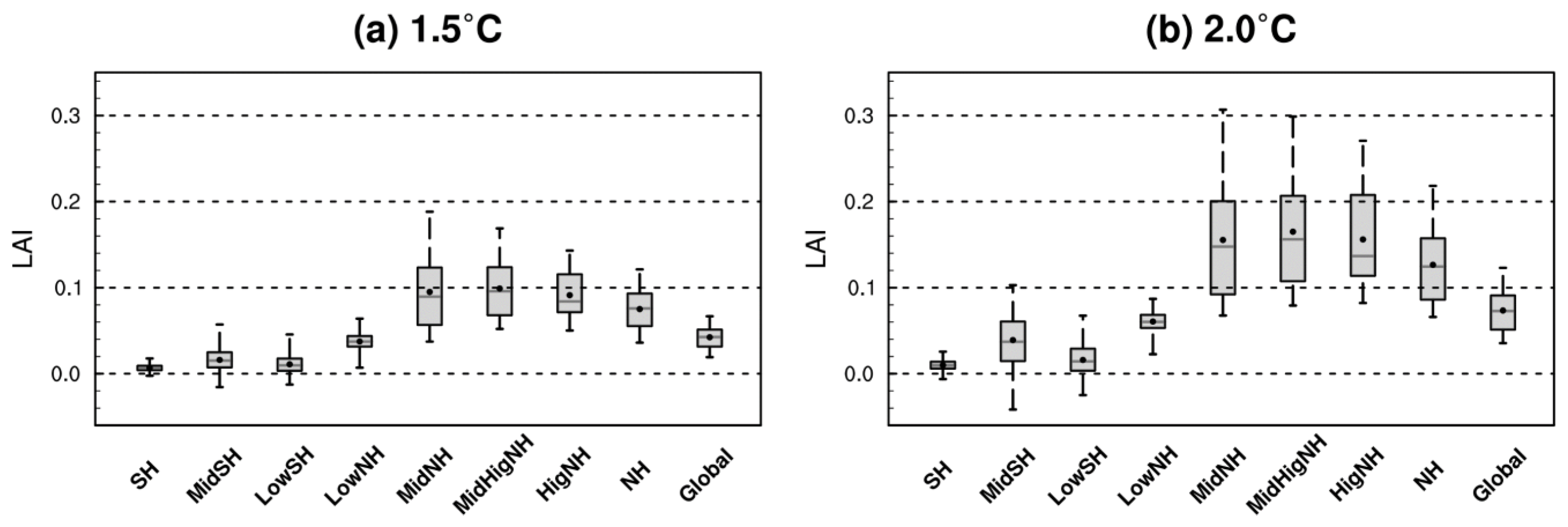
3.2. Future Change of Vegetation Coverage

The increases of near-surface temperature and precipitation in most of the world are conducive to the increases of vegetation density and productivity. LAI is projected to increase and the coverage of bare ground is projected to decrease almost globally except over Brazilian Highland, in which area the decrease of precipitation and near-surface relative humidity are projected (Figure 2d–i). High latitudes in Eurasia are projected to increase the most in terms of the vegetation density and could increase more from 1.5 °C to 2.0 °C of warming (Figure 5a–c). In response to the elevated temperature and precipitation, a poleward expansion of trees into northern Russia and northern Canada is evident (Figure 6). The projected increase of LAI in the high latitudes of the Northern Hemisphere is related to the expansion of tree and grass coverages in areas around 60° N. Apart from the conversion of grasses to trees, the decrease of snow coverage (figure not shown) in areas north to 60° N may also contribute to the increase of vegetation density.
The zonal averages of future changes in LAI, and tree, grass, and bare ground coverages show that the increase and expansion of changes are basically greater with additional 0.5 °C warming than those in the 1.5 °C warming world. All experiments agree with the increase of LAI and decrease of bare ground coverage in the high-latitude zone north to 60° N. However, there are large uncertainties for the future change of LAI in the Southern Hemisphere and tree coverage in both hemispheres between CMIP5 ESMs under low and high GHG emission scenarios. Simulations under RCP2.6 and RCP4.5 scenarios even show opposite future changes of LAI and tree coverages in the low latitudes. This may suggest the high uncertainties of the dynamic vegetation models in simulating the vegetation type change. Compared to the CMIP5, CMIP6 ESMs show higher degree of consistency in the future changes of LAI and vegetation coverages under different scenarios. It is very likely due to the use of vegetation type dataset from LUH2 or a prescribed potential vegetation distribution in half of the CMIP6 models.
Overall, global LAI is projected to increase by 0.04 ± 0.02 and 0.08 ± 0.04 in the 1.5 and 2.0 °C warming worlds respectively. The largest zonal average is in 45–90° N with the projected increments of 0.11 ± 0.06 and 0.19 ± 0.11 respectively (Figure 7). The greening in areas between 45° N and 90° N is related to the increases of tree (0.67 ± 0.19% for 1.5 °C, 0.95 ± 0.39% for 2.0 °C) and grass (0.30 ± 0.18% for 1.5 °C, 0.88 ± 0.22% for 2.0 °C) coverages, accompanied with −0.93 ± 0.35% and −1.03 ± 0.37% of changes, respectively, in bare ground coverage there. It is noteworthy that the change of tree coverage is larger than that of grass in areas between 30° N and 60° N under the 1.5 °C warming level, but less under the 2.0 °C warming level (Figure 8). The interquartile range of LAI and vegetation coverage is smaller in the 1.5 °C warming world than 2.0 °C, representing a better centralization.
Considering the future changes of LAI vary from region to region, six areas from the tropical to sub-arctic zone were selected to investigate the monthly variations of future changes (Figure 9). The monthly variations of climate variables have been shown by Figure 4. Generally, the seasonality of LAI is projected to change little except a small advance of peak time in EUSA. Noted that the CMIP5 and CMIP6 models are not consistent on the sign of future changes of LAI with several exceptions. It is found from Figure 9 that CMIP5 model results contribute a large portion of the future increase of LAI in northeastern Asia, eastern Europe, and eastern US, in which places the CMIP6 model prone to project little change or even decrease of LAI. The CMIP5 and CMIP6 models show opposite sign of future changes in LAI in Brazilian Highland.

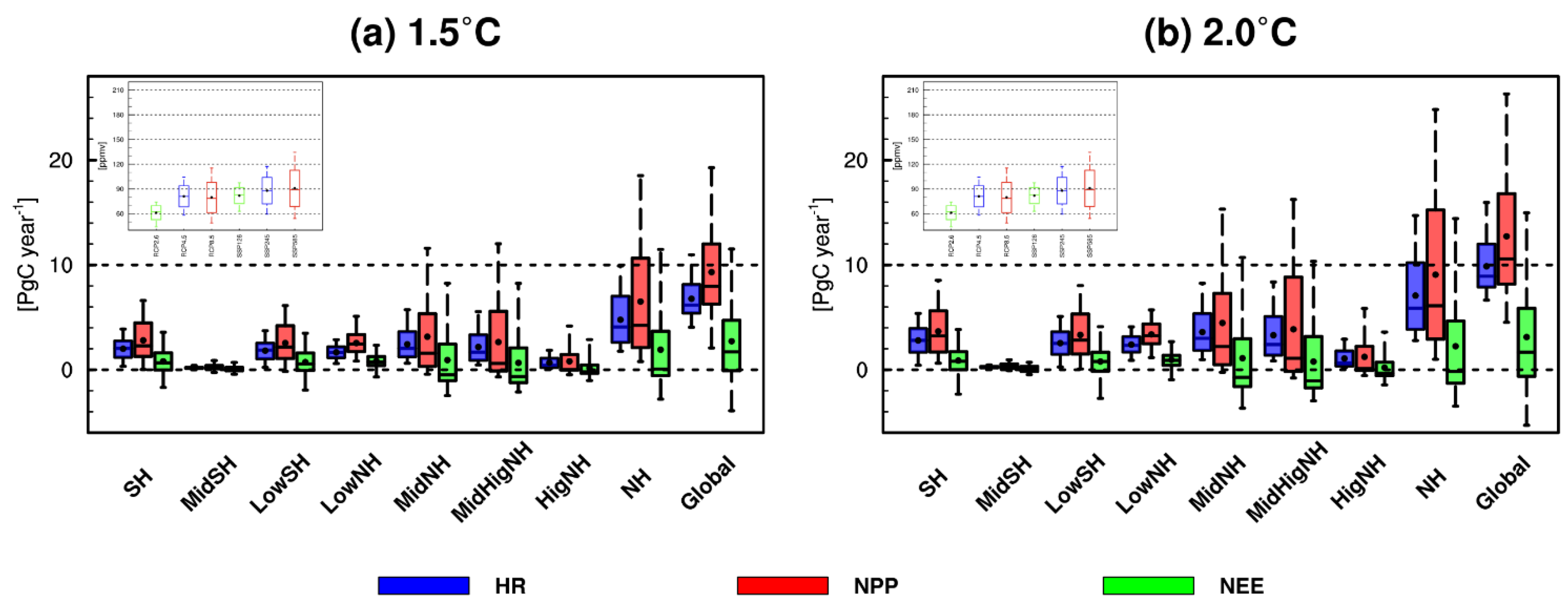
3.3. Future Changes of Terrestrial Carbon Fluxes

The terrestrial carbon fluxes are projected to change accordingly. Figure 10a–f show that NPP and HR are projected to increase globally under global warming except the bare areas. NPP is projected to increase in the high latitudes of Northern Hemisphere, which is related to the expansion of tree and grass coverages and increase of LAI in areas around 60° N. NEE is projected to increase over most of the world except some small areas in Amazon and Brazilian Highland, even though a large proportion of the Amazon and Africa is projected to have a decrease of vegetation coverage (Figure 6). The terrestrial ecosystem could be a stronger carbon sink in the warming world than present, but some areas in Amazon and Central Africa could be stronger carbon sources in a world with additional 0.5 °C warming (Figure 10g–i). It can be seen from the zonal averages of carbon fluxes that the simulation consistency of CMIP5 and CMIP6 on carbon flux changes is higher at 1.5 °C warming level than that at 2.0 °C warming level. But large uncertainty is found for the projected NEE in the tropical zone and Southern Hemisphere by CMIP5 models.
The ensemble global averaged changes of total HR, NPP, and NEE are projected to increase by 7.51 ± 3.46, 10.68 ± 8.60 and 3.80 ± 7.72 PgC year−1 respectively in the 1.5 °C warming world and 11.30 ± 4.66, 15.42 ± 10.90 and 4.83 ± 10.13 PgC year−1 respectively at 2.0 °C warming level (Figure 11). The magnitudes of increases and extensions of changes basically are larger in the 2.0 °C warming world than the 1.5 °C warming world. Distribution of the projected changes are left-skewed generally when global average temperature hits 1.5 °C and 2.0 °C, with much better discreteness of the data in 1.5 °C warming world. The zonal average in 30–60° N is projected to have the largest future changes in all the three variables of HR (3.17 ± 2.55 PgC year−1 for 1.5 °C, 4.61 ± 3.64 PgC year−1 for 2.0 °C), NPP (5.58 ± 6.01 PgC year−1 for 1.5 °C, 7.54 ± 7.78 PgC year−1 for 2.0 °C), and NEE (2.89 ± 5.36 PgC year−1 for 1.5 °C, 3.52 ± 7.19 PgC year−1 for 2.0 °C), followed by areas 45–90° N. Terrestrial in the Northern Hemisphere is projected to be a stronger carbon sink than the Southern Hemisphere, which is due to the noticeable increase of vegetation in the mid-latitudes of Northern Hemisphere (Figure 6).
The monthly variations of total carbon flux changes are shown in Figure 12. The peak NPP is projected to be reached earlier by less than one month from the tropics to the high-latitude, suggesting the growing season is prompted earlier than present. The largest increase of NPP is projected in June while the largest increase of HR is projected in July in EA. Therefore, the largest increase of carbon absorption is projected in June there. The peak increase of NEE could be timed early with additional 0.5 °C warming in EU due to the large increase of carbon assimilation in the growing period in May. Meanwhile, stronger carbon sources than present-day level are projected during dormancy period due to the increases of HR through the year. Comparatively speaking, most of the CMIP5 models project increases of vegetation density and productivity from the tropical area to high latitudes of Northern Hemisphere, while some of the CMIP6 models may show slight changes except in Brazilian Highland. The CMIP5-projected magnitudes of increases in carbon fluxes are mostly larger than those by the CMIP6 models.

3.4. Models’ Inconsistencies

To explore the differences of future changes simulated by different ESMs from CMIP5 and CMIP6, the deviation percentages under different GHG scenarios are analyzed. Here the deviation percentage for a specific variable of a specific ESM is calculated by the global averaged future change over land relative to its ensemble mean. As shown in Figure 13, the deviation percentages of the ESMs in the 1.5 °C mostly are persistent in their signs with additional 0.5 °C warming. Relatively large deviations of RH and wind are found for the ESMs compared to those of PR in the two warming worlds. The Hadley family ESMs from CMIP5 and IPSL-CM6A-LR, MPI-ESM1-2-LR and GFDL-ESM4 from CMIP6 show positive deviation in RH, while others generally show negative deviation. ESMs from CMIP5 and CMIP6 mostly show negative deviation in terms of the 10-m wind except the MIROC family ESMs and HadGEM2-CC from CMIP5 and CanESM5, the EC-Earth3 family ESMs and MPI-ESM1-2-LR from CMIP6. Among them, IPSL-CM6A-LR shows totally opposite deviation in Wind at the 1.5 and 2.0 °C level.
The Hadley family ESMs from CMIP5 and IPSL-CM6A-LR and CESM2 from CMIP6 show larger positive deviation and the INM family ESMs show negative deviation in LAI. The IPSL family ESMS using ORCHIDEE and BCC-CSM2-MR using AVIM2 as their dynamic vegetation models project positive deviated NPP and HR from the ensemble means. However, the EC-Earth3 family ESMs using LPJ-Guess as the dynamic vegetation model project much less change of NPP and HR compared to the others. The ESMs using the vegetation functional type map from a prescribed potential vegetation distribution or the dataset of LUH2 still show a large degree of uncertainties, e.g., the INM family model vs. IPSL-CM6A-LR and MPI-ESM1-2-LR. Also, the CMIP6 ESMs show a limited degree on the reduction of uncertainties of the projected carbon fluxes change.
Basically, the deviation percentages have the same signs and similar magnitudes in vegetation coverage and carbon fluxes in the 1.5 °C and 2.0 °C warming world, suggesting the continuous changes of terrestrial vegetation and carbon cycles if the temperature increase persists. Differences in the predicted changes mostly relate to the different dynamic vegetation modules used in the models, indicating the model-dependent performances in simulating vegetation structure and carbon cycles.

4. Discussion

Carbon cycle is an important process linking the terrestrial ecosystem and climate. The carbon budgets and the related mechanisms have always been hot topics for research in the field of climate change and prediction, mitigation, and countermeasures analysis. Results from this study have several important implications.
Although there are uncertainties in the simulation results of the ESMs, our analysis further indicates (almost all the models agree) that the vegetation density and productivity in the northern high latitudes would increase continuously in the 1.5 °C to 2.0 °C warming worlds. In agreement with previous studies [25,55,56], the positive correlationship between vegetation productivity and temperature probably will continue along the same path as in the past 30–40 years. None of the models projects reverse of the correlationship. However, this may be confined by the ESMs’ capability. Careful scrutinization is needed always using up-to-date model results.
Moreover, we compared the change differences of climate, terrestrial vegetations and related carbon fluxes between the 1.5 °C and 2.0 °C warming worlds, as numerous studies on future changes under the background of warming mainly focus on the change itself under climate warming [17,18,19,57], not investigating the differences between different warming backgrounds. Globally, our results further show that the change magnitudes of greening and vegetation productivity are larger with additional 0.5 °C warming across the model ensemble (Figure 5 and Figure 10). However, the simulation consistency of GHG emission scenarios is higher at 1.5 °C than 2.0 °C. Furthermore, we also investigated the regional monthly variations of LAI and carbon fluxes, and found that the start of the growing season in the northern high latitudes is projected to advance earlier by less than one month in 2.0 °C warming level (Figure 9 and Figure 12). Changes in modeled climate, vegetations and carbon fluxes are also influenced by forcings other than CO2 concentration (CMIP’s GHG emission scenarios) and global warming (1.5 °C and 2.0 °C) caused by greenhouse gases, such as aerosol, nitrogen deposition, land use and land cover changes [20,25,58,59,60]. Thereby, we cannot rule out that our projected results are also influenced by changes in those factors. But we are only concerned with future changes in the 1.5 °C and 2.0 °C warming worlds, and their differences in this paper.
Our results emphasize that compared to the CMIP5 ESMs, CMIP6 ESMs incorporate the projected plant functional type map to take more reliable and consistent future land cover change. Also, our analysis indicates that CMIP5 ESMs are the mainly contribution to simulated LAI increase and the CMIP5-projected magnitudes of increases in carbon fluxes are mostly larger than those by the CMIP6 models. However, the projected uncertainties in NPP and HR are diminished little compared to those from CMIP5 ESMs (Figure 13). This may suggest the emergency of improving the model schemes regarding the terrestrial carbon fluxes.

5. Conclusions

This study investigates how terrestrial vegetation and carbon fluxes change under the two warming scenarios (1.5 °C and 2 °C) relevant to the Paris temperature targets. As the ESMs response differs across climate warming, we use the multi-model ensemble average results to predict future changes. Moreover, the differences and uncertainties of projected variables are investigated by analyzing the deviation percentages of the ESMs.
Although the ESMs show a large spread of uncertainties, a consistent increase of near-surface temperature and precipitation is projected in areas around 60° N. Meantime, the boreal expansion of vegetation coverages is projected. The increases of near-surface temperature and precipitation in most parts of the world are conducive to promoting the increases of vegetation density and productivity. The ensemble means suggest that vegetation density is likely to increase globally except in Brazilian Highland mostly due to the decrease of precipitation there. The high latitudes in Eurasia are projected to have stronger increase of LAI in the 2.0 °C warming world compared to that in 1.5 °C warming level caused by the increase of tree coverage. Most of the ESMs show a uniform increase of NPP and NEE except in some sparse vegetation areas. The terrestrial ecosystem over most of the world could be a stronger carbon sink than present. However, some dry areas in Amazon and Central Africa may convert to carbon sources in a world with additional 0.5 °C warming. Due to the important effect of vegetation-temperature feedback in the northern high latitudes, the area with the largest increase of temperature from 1.5 °C to 2.0 °C warming world coincides well with the area with the largest increase of LAI. The increase of LAI may also contribute to the decrease of relative humidity in the middle latitudes of the North Hemisphere.
The deviations in the predicted changes suggested by different ESMs highlight the model-dependent performances in simulating vegetation structure and carbon cycles. Essentially, they show the same signs and similar magnitudes under the warming threshold of 1.5 °C and 2.0 °C. But there are differences in the predicted changes as different dynamic vegetation components used in the models. The Hadley family ESMs, IPSL-CM6A-LR and CESM2 show larger positive deviation and the INM family ESMs show negative deviation in LAI. ESMS from IPSL families using ORCHIDEE and BCC-CSM2-MR using AVIM2 as their dynamic vegetation models project positive deviation of NPP and HR from the ensemble means, while the EC-Earth3 family ESMs using LPJ-Guess project negative deviation.

Author Contributions

Conceptualization, M.Y., H.C. and X.P.; methodology, M.Y. and X.P.; software and validation, X.P.; formal analysis and investigation, X.P. and M.Y.; writing, X.P. and M.Y.; review and editing, X.P., M.Y. and H.C. All authors have read and agreed to the published version of the manuscript.

Funding

This research was funded by the National Natural Science Foundation of China, grant number 41991285, 42075115 and 42021004.

Data Availability Statement

All the CMIP5 and CMIP6 model outputs are obtained downloaded from https://esgf-node.llnl.gov/search/cmip5/, accessed on 1 November 2021, and https://esgf-node.llnl.gov/search/cmip6/, accessed on 1 November 2021.

Acknowledgments

The authors thank the World Climate Research Programme’s working Group on Coupled Modeling, which is responsible for CMIP. The authors would also like to thank the climate modeling groups listed in Table 1 and Table 2 of this paper for producing and making their model output available.

Conflicts of Interest

The authors declare no conflict of interest.

References

  1. Intergovernmental Panel on Climate Change. Climate Change 2013: The Physical Science Basis; Intergovernmental Panel on Climate Change: New York, NY, USA, 2013. [Google Scholar]
  2. Foley, J.A.; DeFries, R.; Asner, G.P.; Barford, C.; Bonan, G.; Carpenter, S.R.; Chapin, F.S.; Coe, M.T.; Daily, G.C.; Gibbs, H.K.; et al. Global consequences of land use. Science 2005, 309, 570–574. [Google Scholar] [CrossRef] [PubMed] [Green Version]
  3. Raupach, M.; Canadell, J.; Le Quéré, C. Anthropogenic and biophysical contributors to increasing atmospheric CO2 growth rate and airborne fraction. Biogeosci. Discuss. 2008, 5, 2867–2896. [Google Scholar] [CrossRef]
  4. Beer, C.; Reichstein, M.; Tomelleri, E.; Ciais, P.; Jung, M.; Carvalhais, N.; Rödenbeck, C.; Arain, M.A.; Baldocchi, D.; Bonan, G.B.; et al. Terrestrial gross carbon dioxide uptake: Global distribution and covariation with climate. Science 2010, 329, 834–838. [Google Scholar] [CrossRef] [PubMed] [Green Version]
  5. Sivakumar, B. Global climate change and its impacts on water resources planning and management: Assessment and challenges. Stoch. Environ. Res. Risk Assess. 2010, 25, 583–600. [Google Scholar] [CrossRef]
  6. Li, L.; Wang, Y.-P.; Beringer, J.; Shi, H.; Cleverly, J.; Cheng, L.; Eamus, D.; Huete, A.; Hutley, L.; Lu, X.; et al. Responses of LAI to rainfall explain contrasting sensitivities to carbon uptake between forest and non-forest ecosystems in Australia. Sci. Rep. 2017, 7, 11720. [Google Scholar] [CrossRef]
  7. Chen, J.M.; Ju, W.; Ciais, P.; Viovy, N.; Liu, R.; Liu, Y.; Lu, X. Vegetation structural change since 1981 significantly enhanced the terrestrial carbon sink. Nat. Commun. 2019, 10, 4259. [Google Scholar] [CrossRef] [PubMed]
  8. Bastin, J.-F.; Finegold, Y.; Garcia, C.; Mollicone, D.; Rezende, M.; Routh, D.; Zohner, C.M.; Crowther, T.W. The global tree restoration potential. Science 2019, 365, 76–79. [Google Scholar] [CrossRef] [PubMed]
  9. Pendergrass, A.G.; Knutti, R.; Lehner, F.; Deser, C.; Sanderson, B. Precipitation variability increases in a warmer climate. Sci. Rep. 2017, 7, 17966. [Google Scholar] [CrossRef] [Green Version]
  10. Dai, A.; Rasmussen, R.M.; Liu, C.; Ikeda, K.; Prein, A.F. A new mechanism for warm-season precipitation response to global warming based on convection-permitting simulations. Clim. Dyn. 2017, 55, 343–368. [Google Scholar] [CrossRef]
  11. Markus, M.; Cai, X.; Sriver, R. Extreme Floods and Droughts under Future Climate Scenarios. Water 2019, 11, 1720. [Google Scholar] [CrossRef] [Green Version]
  12. Nations, U. Adoption of the paris agreement. Conf. Parties Twenty-First Sess. 2015, L.9, 21932. [Google Scholar]
  13. Lee, D.; Min, S.-K.; Fischer, E.M.; Shiogama, H.; Bethke, I.; Lierhammer, L.; Scinocca, J.F. Impacts of half a degree additional warming on the Asian summer monsoon rainfall characteristics. Environ. Res. Lett. 2018, 13, 044033. [Google Scholar] [CrossRef] [Green Version]
  14. Döll, P.; Trautmann, T.; Gerten, D.; Schmied, H.M.; Ostberg, S.; Saaed, F.; Schleussner, C.-F. Risks for the global freshwater system at 1.5 °C and 2 °C global warming. Environ. Res. Lett. 2018, 13, 044038. [Google Scholar] [CrossRef]
  15. Vaughan, N.E.; Gough, C.; Mander, S.; Littleton, E.W.; Welfle, A.; Gernaat, D.E.H.J.; Van Vuuren, D.P. Evaluating the use of biomass energy with carbon capture and storage in low emission scenarios. Environ. Res. Lett. 2018, 13, 044014. [Google Scholar] [CrossRef]
  16. Bittermann, K.; Rahmstorf, S.; Kopp, R.E.; Kemp, A.C. Global mean sea-level rise in a world agreed upon in Paris. Environ. Res. Lett. 2017, 12, 124010. [Google Scholar] [CrossRef]
  17. Rasmussen, D.J.; Bittermann, K.; Buchanan, M.K.; Kulp, S.; Strauss, B.H.; Kopp, R.E.; Oppenheimer, M. Extreme sea level implications of 1.5 °C, 2.0 °C, and 2.5 °C temperature stabilization targets in the 21st and 22nd centuries. Environ. Res. Lett. 2018, 13, 034040. [Google Scholar] [CrossRef]
  18. Aerenson, T.; Tebaldi, C.; Sanderson, B.; Lamarque, J.-F. Changes in a suite of indicators of extreme temperature and precipitation under 1.5 and 2 degrees warming. Environ. Res. Lett. 2018, 13, 035009. [Google Scholar] [CrossRef]
  19. Kong, Y.; Wang, C.-H. Responses and changes in the permafrost and snow water equivalent in the Northern Hemisphere under a scenario of 1.5 °C warming. Adv. Clim. Chang. Res. 2017, 8, 235–244. [Google Scholar] [CrossRef]
  20. Bonan, G.B.; Pollard, D.; Thompson, S.L. Effects of boreal forest vegetation on global climate. Nat. Cell Biol. 1992, 359, 716–718. [Google Scholar] [CrossRef]
  21. Nemani, R.R.; Keeling, C.D.; Hashimoto, H.; Jolly, W.M.; Piper, S.C.; Tucker, C.J.; Myneni, R.B.; Running, S.W. Climate-Driven Increases in Global Terrestrial Net Primary Production from 1982 to 1999. Science 2003, 300, 1560–1563. [Google Scholar] [CrossRef] [Green Version]
  22. Martinez, C.; Bianconi, M.; Silva, L.; Approbato, A.; Lemos, M.; Santos, L.; Curtarelli, L.; Rodrigues, A.; Mello, T.; Manchon, F. Moderate warming increases PSII performance, antioxidant scavenging systems and biomass production in Stylosanthes capitata Vogel. Environ. Exp. Bot. 2014, 102, 58–67. [Google Scholar] [CrossRef]
  23. Linderholm, H.W. Growing season changes in the last century. Agric. For. Meteorol. 2006, 137, 1–14. [Google Scholar] [CrossRef]
  24. Bauweraerts, I.; Wertin, T.M.; Ameye, M.; McGuire, M.A.; Teskey, R.O.; Steppe, K. The effect of heat waves, elevated [CO2] and low soil water availability on northern red oak (Quercus rubraL.) seedlings. Glob. Chang. Biol. 2012, 19, 517–528. [Google Scholar] [CrossRef]
  25. Piao, S.; Wang, X.; Park, T.; Chen, C.; Lian, X.; He, Y.; Bjerke, J.; Chen, A.; Ciais, P.; Tømmervik, H.; et al. Characteristics, drivers and feedbacks of global greening. Nat. Rev. Earth Environ. 2019, 1, 14–27. [Google Scholar] [CrossRef]
  26. Mao, J.; Shi, X.; Thornton, P.E.; Hoffman, F.M.; Zhu, Z.; Myneni, R.B. Global Latitudinal-Asymmetric Vegetation Growth Trends and Their Driving Mechanisms: 1982–2009. Remote Sens. 2013, 5, 1484–1497. [Google Scholar] [CrossRef] [Green Version]
  27. Xia, J.; Chen, J.; Piao, S.; Ciais, P.; Luo, Y.; Wan, S. Terrestrial carbon cycle affected by non-uniform climate warming. Nat. Geosci. 2014, 7, 173–180. [Google Scholar] [CrossRef]
  28. Yue, X.; Liao, H.; Wang, H.; Zhang, T.; Unger, N.; Sitch, S.; Feng, Z.; Yang, J. Pathway dependence of ecosystem responses in China to 1.5 °C global warming. Atmos. Chem. Phys. Discuss. 2020, 20, 2353–2366. [Google Scholar] [CrossRef] [Green Version]
  29. El Masri, B.; Schwalm, C.; Huntzinger, D.N.; Mao, J.; Shi, X.; Peng, C.; Fisher, J.B.; Jain, A.K.; Tian, H.; Poulter, B.; et al. Carbon and Water Use Efficiencies: A Comparative Analysis of Ten Terrestrial Ecosystem Models under Changing Climate. Sci. Rep. 2019, 9, 14680. [Google Scholar] [CrossRef] [Green Version]
  30. Friedlingstein, P.; Meinshausen, M.; Arora, V.K.; Jones, C.D.; Anav, A.; Liddicoat, S.K.; Knutti, R. Uncertainties in CMIP5 Climate Projections due to Carbon Cycle Feedbacks. J. Clim. 2014, 27, 511–526. [Google Scholar] [CrossRef] [Green Version]
  31. Huntzinger, D.N.; Michalak, A.M.; Schwalm, C.; Ciais, P.; King, A.W.; Fang, Y.; Schaefer, K.; Wei, Y.; Cook, R.B.; Fisher, J.B.; et al. Uncertainty in the response of terrestrial carbon sink to environmental drivers undermines carbon-climate feedback predictions. Sci. Rep. 2017, 7, 4765. [Google Scholar] [CrossRef]
  32. Yu, M.; Wang, G.; Chen, H. Quantifying the impacts of land surface schemes and dynamic vegetation on the model dependency of projected changes in surface energy and water budgets. J. Adv. Model. Earth Syst. 2016, 8, 370–386. [Google Scholar] [CrossRef] [Green Version]
  33. Dong, T.; Dong, W. Evaluation of extreme precipitation over Asia in CMIP6 models. Clim. Dyn. 2021, 57, 1751–1769. [Google Scholar] [CrossRef]
  34. Jiang, J.H.; Su, H.; Wu, L.; Zhai, C.; Schiro, K.A. Improvements in Cloud and Water Vapor Simulations Over the Tropical Oceans in CMIP6 Compared to CMIP5. Earth Space Sci. 2021, 8, e2020EA001520. [Google Scholar] [CrossRef]
  35. Bracegirdle, T.J.; Holmes, C.R.; Hosking, J.S.; Marshall, G.; Osman, M.; Patterson, M.; Rackow, T. Improvements in Circumpolar Southern Hemisphere Extratropical Atmospheric Circulation in CMIP6 Compared to CMIP5. Earth Space Sci. 2020, 7, e2019EA001065. [Google Scholar] [CrossRef]
  36. Hurtt, G.C.; Chini, L.; Sahajpal, R.; Frolking, S.; Bodirsky, B.L.; Calvin, K.; Doelman, J.C.; Fisk, J.; Fujimori, S.; Goldewijk, K.K.; et al. Harmonization of global land use change and management for the period 850–2100 (LUH2) for CMIP6. Geosci. Model. Dev. 2020, 13, 5425–5464. [Google Scholar] [CrossRef]
  37. Dufresne, J.-L.; Foujols, M.-A.; Denvil, S.; Caubel, A.; Marti, O.; Aumont, O.; Balkanski, Y.; Bekki, S.; Bellenger, H.; Benshila, R.; et al. Climate change projections using the IPSL-CM5 Earth System Model: From CMIP3 to CMIP5. Clim. Dyn. 2013, 40, 2123–2165. [Google Scholar] [CrossRef]
  38. Watanabe, S.; Hajima, T.; Sudo, K.; Nagashima, T.; Takemura, T.; Okajima, H.; Nozawa, T.; Kawase, H.; Abe, M.; Yokohata, T.; et al. MIROC-ESM 2010: Model description and basic results of CMIP5-20c3m experiments. Geosci. Model Dev. 2011, 4, 845–872. [Google Scholar] [CrossRef] [Green Version]
  39. Martin, G.M.; Bellouin, N.; Collins, W.J.; Culverwell, I.D.; Halloran, P.R.; Hardiman, S.C.; Hinton, T.J.; Jones, C.D.; McDonald, R.E.; McLaren, A.J.; et al. The HadGEM2 family of Met Office Unified Model climate configurations. Geosci. Model Dev. 2011, 4, 723–757. [Google Scholar] [CrossRef] [Green Version]
  40. Raddatz, T.; Reick, C.; Knorr, W.; Kattge, J.; Roeckner, E.; Schnur, R.; Schnitzler, K.-G.; Wetzel, P.; Jungclaus, J. Will the tropical land biosphere dominate the climate—Carbon cycle feedback during the 21st century? Clim. Dyn. 2007, 29, 565–574. [Google Scholar] [CrossRef]
  41. Reick, C.H.; Raddatz, T.; Brovkin, V.; Gayler, V. Representation of natural and anthropogenic land cover change in MPI-ESM. J. Adv. Model. Earth Syst. 2013, 5, 459–482. [Google Scholar] [CrossRef]
  42. Dunne, J.P.; John, J.G.; Shevliakova, E.; Stouffer, R.J.; Krasting, J.; Malyshev, S.L.; Milly, P.C.D.; Sentman, L.T.; Adcroft, A.J.; Cooke, W.; et al. GFDL’s ESM2 Global Coupled Climate–Carbon Earth System Models. Part II: Carbon System Formulation and Baseline Simulation Characteristics. J. Clim. 2013, 26, 2247–2267. [Google Scholar] [CrossRef] [Green Version]
  43. Li, W.; Zhang, Y.; Shi, X.; Zhou, W.; Huang, A.; Mu, M.; Qiu, B.; Ji, J. Development of Land Surface Model BCC_AVIM2.0 and Its Preliminary Performance in LS3MIP/CMIP6. J. Meteorol. Res. 2019, 33, 851–869. [Google Scholar] [CrossRef]
  44. Wu, T.; Lu, Y.; Fang, Y.; Xin, X.; Li, L.; Li, W.; Jie, W.; Zhang, J.; Liu, Y.; Zhang, L.; et al. The Beijing Climate Center Climate System Model (BCC-CSM): The main progress from CMIP5 to CMIP6. Geosci. Model Dev. 2019, 12, 1573–1600. [Google Scholar] [CrossRef] [Green Version]
  45. Swart, N.C.; Cole, J.N.S.; Kharin, V.V.; Lazare, M.; Scinocca, J.F.; Gillett, N.P.; Anstey, J.; Arora, V.; Christian, J.R.; Hanna, S.; et al. The Canadian Earth System Model version 5 (CanESM5.0.3). Geosci. Model Dev. 2019, 12, 4823–4873. [Google Scholar] [CrossRef] [Green Version]
  46. Wyser, K.; van Noije, T.; Yang, S.; von Hardenberg, J.; O’Donnell, D.; Döscher, R. On the increased climate sensitivity in the EC-Earth model from CMIP5 to CMIP6. Geosci. Model Dev. 2020, 13, 3465–3474. [Google Scholar] [CrossRef]
  47. Volodin, E.M. Atmosphere-ocean general circulation model with the carbon cycle. Izv. Atmos. Ocean. Phys. 2007, 43, 266–280. [Google Scholar] [CrossRef]
  48. Volodin, E.M.; Mortikov, E.; Kostrykin, S.V.; Galin, V.Y.; Lykossov, V.N.; Gritsun, A.; Diansky, N.A.; Gusev, A.V.; Iakovlev, N.; Shestakova, A.A.; et al. Simulation of the modern climate using the INM-CM48 climate model. Russ. J. Numer. Anal. Math. Model. 2018, 33, 367–374. [Google Scholar] [CrossRef]
  49. Lurton, T.; Balkanski, Y.; Bastrikov, V.; Bekki, S.; Bopp, L.; Braconnot, P.; Brockmann, P.; Cadule, P.; Contoux, C.; Cozic, A.; et al. Implementation of the CMIP6 Forcing Data in the IPSL-CM6A-LR Model. J. Adv. Model. Earth Syst. 2020, 12, e2019MS001940. [Google Scholar] [CrossRef] [Green Version]
  50. Boucher, O.; Servonnat, J.; Albright, A.L.; Aumont, O.; Balkanski, Y.; Bastrikov, V.; Bekki, S.; Bonnet, R.; Bony, S.; Bopp, L.; et al. Presentation and Evaluation of the IPSL-CM6A-LR Climate Model. J. Adv. Model. Earth Syst. 2020, 12, e2019MS002010. [Google Scholar] [CrossRef]
  51. Mauritsen, T.; Bader, J.; Becker, T.; Behrens, J.; Bittner, M.; Brokopf, R.; Brovkin, V.; Claussen, M.; Crueger, T.; Esch, M.; et al. Developments in the MPI-M Earth System Model version 1.2 (MPI-ESM1.2) and Its Response to Increasing CO 2. J. Adv. Model. Earth Syst. 2019, 11, 998–1038. [Google Scholar] [CrossRef] [Green Version]
  52. Lawrence, D.M.; Fisher, R.A.; Koven, C.D.; Oleson, K.W.; Swenson, S.C.; Bonan, G.; Collier, N.; Ghimire, B.; van Kampenhout, L.; Kennedy, D.; et al. The Community Land Model Version 5: Description of New Features, Benchmarking, and Impact of Forcing Uncertainty. J. Adv. Model. Earth Syst. 2019, 11, 4245–4287. [Google Scholar] [CrossRef] [Green Version]
  53. Gettelman, A.; Hannay, C.; Bacmeister, J.T.; Neale, R.B.; Pendergrass, A.G.; Danabasoglu, G.; Lamarque, J.; Fasullo, J.T.; Bailey, D.A.; Lawrence, D.M.; et al. High Climate Sensitivity in the Community Earth System Model Version 2 (CESM2). Geophys. Res. Lett. 2019, 46, 8329–8337. [Google Scholar] [CrossRef]
  54. Dunne, J.P.; Horowitz, L.W.; Adcroft, A.J.; Ginoux, P.; Held, I.M.; John, J.G.; Krasting, J.P.; Malyshev, S.; Naik, V.; Paulot, F.; et al. The GFDL Earth System Model Version 4.1 (GFDL-ESM 4.1): Overall Coupled Model Description and Simulation Characteristics. J. Adv. Model. Earth Syst. 2020, 12, e2019MS002015. [Google Scholar] [CrossRef]
  55. Knapp, A.K.; Smith, M.D. Variation among Biomes in Temporal Dynamics of Aboveground Primary Production. Science 2001, 291, 481–484. [Google Scholar] [CrossRef] [PubMed] [Green Version]
  56. Running, S.W.; Nemani, R.R.; Heinsch, F.A.; Zhao, M.; Reeves, M.; Hashimoto, H. A Continuous Satellite-Derived Measure of Global Terrestrial Primary Production. Bioscience 2004, 54, 547–560. [Google Scholar] [CrossRef]
  57. Tobin, I.; Greuell, W.; Jerez, S.; Ludwig, F.; Vautard, R.; van Vliet, M.T.; Bréon, F.-M. Vulnerabilities and resilience of European power generation to 1.5 °C, 2 °C and 3 °C warming. Environ. Res. Lett. 2018, 13, 044024. [Google Scholar] [CrossRef]
  58. Wang, Z.; Lin, L.; Zhang, X.; Zhang, H.; Liu, L.; Xu, Y. Scenario dependence of future changes in climate extremes under 1.5 °C and 2 °C global warming. Sci. Rep. 2017, 7, 46432. [Google Scholar] [CrossRef] [PubMed]
  59. Haberl, H.; Erb, K.; Krausmann, F.; Gaube, V.; Bondeau, A.; Plutzar, C.; Gingrich, S.; Lucht, W.; Fischer-Kowalski, M. Quantifying and mapping the human appropriation of net primary production in earth’s terrestrial ecosystems. Proc. Natl. Acad. Sci. USA 2007, 104, 12942–12947. [Google Scholar] [CrossRef] [Green Version]
  60. Samset, B.H.; Sand, M.; Smith, C.J.; Bauer, S.E.; Forster, P.M.; Fuglestvedt, J.S.; Osprey, S.; Schleussner, C. Climate Impacts From a Removal of Anthropogenic Aerosol Emissions. Geophys. Res. Lett. 2018, 45, 1020–1029. [Google Scholar] [CrossRef] [PubMed] [Green Version]
Figure 1. 20-year analysis period of each model under different GHG emission scenarios when (a) 1.5 °C and (b) 2.0 °C warming level is reached.
Atmosphere 13 00042 g001
Figure 2. Future changes of 2-m temperature (ac, in °C), precipitation (df, in mm/day), near-surface relative humidity (gi, in %) and 10-m wind speed (jl, in m/s) simulated by the selected ESMs at the warming level of 1.5 °C (left column) and 2.0 °C (middle column) with their zonal averages showing on the right. Their differences are in the right column. Only areas where the S/NTAS > 5 or S/N > 1 for PR, RH, and wind are shaded.
Atmosphere 13 00042 g002
Figure 3. The boxplots of future changes of 2-m temperature (in °C), precipitation (in mm/day), near-surface relative humidity (in %) and 10-m wind speed (in m/s) in different latitude zones over land (SH: 0–90° S, MidSH: 30–60° S, LowSH: 0–30° S, LowNH: 0–30° N, MidNH: 30–60° N, MidHigNH: 45–90° N, HigNH: 60–90° N, NH: 0–90° N, Global: 90° S–90° N) under the warming threshold of 1.5 °C and 2.0 °C. The whiskers mean the maximum and minimum, the lines of boxes mean the 1st quantile, median, and 3rd quantile of values, and the dots show the averages.
Atmosphere 13 00042 g003
Figure 4. Scenario-dependent monthly variations (in lines and right y-axis) and the ensemble average of future changes (in bars and left y-axis) in 2-m temperature (in °C), precipitation (in mm/day), near-surface relative humidity (in %) and 10-m wind speed (in m/s) in the areas of EA, EU, Congo, EUSA, Amzn1, and Amzn2. The selected areas are shown by the squares plotted in Figure 5a.
Atmosphere 13 00042 g004
Figure 5. Future changes of LAI (ac) simulated by the selected ESMs at the warming level of 1.5 °C (left column) and 2.0 °C (middle column) with their zonal averages showing on the right. Their differences are in the right column. Only areas where the S/N > 1 are shaded. The red rectangles boxes in a show the selected areas (EA: northeastern Asia, EU: eastern Europe, Congo Basin, EUSA: eastern US, Amzn1: Amazon, Amzn2: Brazilian Highland) to investigate the monthly variations of future changes.
Atmosphere 13 00042 g005
Figure 6. Future changes of tree (ac, in %), grass (df, in %), and bare soil (gi, in %) coverages simulated by the selected ESMs at the warming level of 1.5 °C (left column) and 2.0 °C (middle column) with their zonal averages showing on the right. Their differences are in the right column. Only areas where the S/N > 1 are shaded.
Atmosphere 13 00042 g006
Figure 7. The boxplots of future changes of LAI in different latitude zones (SH: 0–90° S, MidSH: 30–60° S, LowSH: 0–30° S, LowNH: 0–30° N, MidNH: 30–60° N, MidHigNH: 45–90° N, HigNH: 60–90° N, NH: 0–90° N, Global: 90° S–90° N) under the warming threshold of 1.5 °C and 2.0 °C. The whiskers mean the maximum and minimum, the lines of boxes mean the 1st quantile, median, and 3rd quantile of values, and the dots show the averages.
Atmosphere 13 00042 g007
Figure 8. The boxplots of future changes in coverages of tree, grass, and bare soil (in %) in different latitude zones (SH: 0–90° S, MidSH: 30–60° S, LowSH: 0–30° S, LowNH: 0–30° N, MidNH: 30–60° N, MidHigNH: 45–90° N, HigNH: 60–90° N, NH: 0–90° N, Global: 90° S–90° N) under the warming threshold of 1.5 °C and 2.0 °C. The whiskers mean the maximum and minimum, the lines of boxes mean the 1st quantile, median, and 3rd quantile of values, and the dots show the averages.
Atmosphere 13 00042 g008
Figure 9. Scenario-dependent monthly variations (in lines and right y-axis) and the ensemble average of future changes (in bars and left y-axis) in LAI in the areas of EA, EU, Congo, EUSA, Amzn1 and Amzn2. The selected areas are shown by the squares plotted in Figure 5a.
Atmosphere 13 00042 g009
Figure 10. Future changes of NPP (ac, in kgC m−2 year−1), HR (df, in kgC m−2 year−1) and NEE (gi, in kgC m−2 year−1) simulated by the selected ESMs at the warming level of 1.5 °C (left column) and 2.0 °C (middle column) with their zonal averages showing on the right. Their differences are in the right column. Only areas where the S/NNPP > 2 or S/NHR > 2 or S/NNEE > 1 are shaded.
Atmosphere 13 00042 g010
Figure 11. The boxplots of future changes in total terrestrial HR, NPP, and NEE (in PgC year−1) in different latitude zones (SH: 0–90° S, MidSH: 30–60° S, LowSH: 0–30° S, LowNH: 0–30° N, MidNH: 30–60° N, MidHigNH: 45–90° N, HigNH: 60–90° N, NH: 0–90° N, Global: 90° S–90° N) under the warming threshold of 1.5 °C and 2.0 °C. The whiskers mean the maximum and minimum, the lines of boxes mean the 1st quantile, median and 3rd quantile of values, and the dots show the averages. The attached picture in the upper left corner shows the increase range of CO2 concentration data under different emission concentration paths.
Atmosphere 13 00042 g011
Figure 12. Scenario-dependent monthly variations (in lines and right y-axis) and the ensemble average of future changes (in bars and left y-axis) in total NPP, HR, and NEE (in PgC year−1) in the areas of EA, EU, Congo, EUSA, Amzn1, and Amzn2. The selected areas are shown by the squares plotted in Figure 5a.
Atmosphere 13 00042 g012
Figure 13. Deviation percentages relative to the ensemble averages of future changes over land under RCP2.6/SSP126 (left triangle), RCP4.5/SSP245 (top triangle), and RCP8.5/SSP585 (right triangle) scenarios, and their averages (bottom triangle) in the 1.5 °C (a) and 2.0 °C (b) warming world. Gray represents the unavailability of model output.
Atmosphere 13 00042 g013
Table 1. Basic information of the CMIP5 ESMs.
CMIPModelsLand ModelsDynamic VegetationOriginal Resolution (lat × lon)Emission Scenarios
(1.5 °C)
Emission Scenarios
(2.0 °C)
References
RCP2.6RCP4.5RCP8.5RCP2.6RCP4.5RCP8.5
CMIP5IPSL-CM5A-LRORCHIDEEORCHIDEE96 × 96 [37]
IPSL-CM5B-LRORCHIDEEORCHIDEE96 × 96 [37]
MIROC-ESMMATSIRO + SEIB-DGVMSEIB-DGVM64 × 128[38]
MIROC-ESM-CHEMMATSIRO + SEIB-DGVMSEIB-DGVM64 × 128[38]
HadGEM2-CCMOSES2 + TRIFFIDTRIFFID145 × 192 [39]
HadGEM2-ESMOSES2 + TRIFFIDTRIFFID145 × 192[39]
MPI-ESM-LRJSBACH + BETHYDYNVEG [40]96 × 192 [41]
MPI-ESM-MRJSBACH + BETHYDYNVEG96 × 192 [41]
GFDL-ESM2GLM3LM390 × 144 [42]
GFDL-ESM2MLM3LM390 × 144 [42]
Note: ‘√’ indicates the availability of model output in the world of 1.5 °C or 2.0 °C warming level.
Table 2. Basic information of the CMIP6 ESMs.
CMIPModelsLand ModelsDynamic VegetationOriginal Resolution (lat × lon)Emission Scenarios
(1.5 °C)
Emission Scenarios
(2.0 °C)
References
SSP126SSP245SSP585SSP126SSP245SSP585
CMIP6BCC-CSM2-MRBCC-AVIM2AVIM2.0 [43]160 × 320 [44]
CanESM5CLASS3.6 + CTEM1.2CTEM1.264 × 128[45]
EC-Earth3-CCHTESSEL + LPJ-GUESS v4LPJ-Guess256 × 512 [46]
EC-Earth3-VegHTESSEL + LPJ-GUESS v4LPJ-Guess256 × 512[46]
INM-CM4-8INM-LND1“A carbon cycle module [47] with prescribed potential vegetation distribution and root-zone soil moisture determined actual vegetation.”120 × 180 [48]
INM-CM5-0INM-LND1120 × 180 [48]
IPSL-CM6A-LRORCHIDEEThe land cover maps specific for simulations using reference data sets for CMIP6 within the LUH2 database [49].143 × 144[50]
MPI-ESM1-2-LRJSBACH3.20JSBACH uses the LUH2 data set to simulate land use change.96 × 192 [51]
CESM2CLM5CLM5 combines updated versions of current day satellite land cover descriptions with the LUH2 data (Lawrence et al., 2019) [52].192 × 288[53]
GFDL-ESM4GFDL-LM4.1LM4.1180 × 288 [54]
Note: ‘√’ indicates the availability of model output in the world of 1.5 °C or 2.0 °C warming level.
Publisher’s Note: MDPI stays neutral with regard to jurisdictional claims in published maps and institutional affiliations.

