Assessment of 13 Gridded Precipitation Datasets for Hydrological Modeling in a Mountainous Basin

Abstract

Precipitation measurement with high spatial and temporal resolution over highly elevated and complex terrain in the eastern part of Turkey is an essential task to manage the water structures in an optimum manner. The objective of this study is to evaluate the consistency and hydrologic utility of 13 Gridded Precipitation Datasets (GPDs) (CPCv1, MSWEPv2.8, ERA5, CHIRPSv2.0, CHIRPv2.0, IMERGHHFv06, IMERGHHEv06, IMERGHHLv06, TMPA-3B42v7, TMPA-3B42RTv7, PERSIANN-CDR, PERSIANN-CCS, and PERSIANN) over a mountainous test basin (Karasu) at a daily time step. The Kling-Gupta Efficiency (KGE), including its three components (correlation, bias, and variability ratio), and the Nash-Sutcliffe Efficiency (NSE) are used for GPD evaluation. Moreover, the Hanssen-Kuiper (HK) score is considered to evaluate the detectability strength of selected GPDs for different precipitation events. Precipitation frequencies are evaluated considering the Probability Density Function (PDF). Daily precipitation data from 23 meteorological stations are provided as a reference for the period of 2015–2019. The TUW model is used for hydrological simulations regarding observed discharge located at the outlet of the basin. The model is calibrated in two ways, with observed precipitation only and by each GPD individually. Overall, CPCv1 shows the highest performance (median KGE; 0.46) over time and space. MSWEPv2.8 and CHIRPSv2.0 deliver the best performance among multi-source merging datasets, followed by CHIRPv2.0, whereas IMERGHHFv06, PERSIANN-CDR, and TMPA-3B42v7 show poor performance. IMERGHHLv06 is able to present the best performance (median KGE; 0.17) compared to other satellite-based GPDs (PERSIANN-CCS, PERSIANN, IMERGHHEv06, and TMPA-3B42RTv7). ERA5 performs well both in spatial and temporal validation compared to satellite-based GPDs, though it shows low performance in producing a streamflow simulation. Overall, all gridded precipitation datasets show better performance in generating streamflow when the model is calibrated by each GPD separately.

1. Introduction

Precipitation data with high spatial and temporal resolution is one of the key components for hydrological modeling [1,2]. Though the inconsistency of precipitation over space and scarcity of ground-based gauge observation, especially over a basin with complex topography, significantly affect the rainfall-runoff simulation process [3,4]. Various methods have been used for precipitation estimates and each of them has its pros and cons. Ground-based gauge networks measure precipitation directly, but the spatial variability of precipitation over time is highly dependent on the density of the gauge network [5,6]. Moreover, technical issues in developing countries and problems such as information exchange and data sharing for transboundary river basins have brought significant challenges to obtaining gauge precipitation data [7]. Ground weather radars are able to present precipitation estimates with high spatial and temporal resolution, however, the complexity of the terrain, limited spatial range, and indirect measurement of precipitation present several errors and uncertainties in radar-based precipitation estimates [8,9,10]. In recent decades, remote sensing and data assimilation technology have developed rapidly. The space-borne sensors and numerical weather prediction models are able to present a variety of Gridded Precipitation Datasets (GPDs) in different spatial and temporal resolutions with nearly global coverage [11,12]. Satellite-based and numerical weather prediction model precipitation estimates can be considered as an alternative to fill the spatio-temporal gaps of ground-based networks, especially over complex topography where gauge network is scarce. However, the presence of high bias in some of these gridded precipitation datasets is one of the factors which limit their application for hydrological modeling [13].

Hydrological models are used to simplify the real-world problems related to the water cycle and water resources management or to consider only relevant information instead of simulating every realistic scenario for a better understanding of basin characteristics [14,15]. Therefore, the number and complexity of hydrological models have increased to support various decisions regarding management policies related to water resources management, climate change, and land use. Simple models need fewer input data, are easy to calibrate the model parameters, and are able to process quickly, while the complexity of the model increases the level of information as input for the model and provides consideration of diverse issues in water resources management [16,17]. River discharge is one of the important hydrologic components and its estimation at a particular location could be necessary for the design and management of different water resource structures [18,19]. Rainfall-runoff models provide the opportunity to simulate streamflow based on observed precipitation or using Gridded Precipitation Datasets (GPDs) as meteorological forcing and can be compared with observed discharge to evaluate their hydrologic utility [20]. In this study, we performed both meteorological and hydrological evaluation of several GPDs and assumed the observed streamflow data are the best available estimates.

Generally, two types of validation methodologies are used to quantify the performance of GPDs: (1) direct comparison of precipitation datasets with a ground-based gauge network or radar-based precipitation estimates (meteorological evaluation); and (2) validation of Gridded Precipitation Datasets (GPDs) using hydrological models to evaluate their strength in streamflow prediction (hydrological evaluation) [21].

Many authors have reported the validation of different gridded precipitation datasets over various regions [1,22,23,24,25,26,27,28,29,30]. However, the validation and consistency of GPDs for a certain area may not be applicable in others, so a separate assessment is necessary to address their reliability over that particular region.

There are also a number of studies evaluating the performance of certain GPDs over all or selected regions of Turkey [31,32,33,34,35,36,37,38,39]. However, in these investigations, either a limited number or old versioned GPDs have been tested which mainly consider meteorological performance in a coarse monthly time step instead of daily. Thus, we see the necessity of a more comprehensive study to include both meteorological and hydrological performance of GPDs with a finer time step (daily) and to consider seasonal effects.

This study aims to evaluate the spatio-temporal consistency of 13 GPDs by considering the entire period and seasonal variability of precipitation as well as testing the hydrological utility based on two different scenarios (Scheme-1 and Scheme-2) over a complex topography used for different scientific research projects in Turkey. The structure of this paper is as follows: Section 1 presents a comprehensive introduction to GPDs. Section 2 gives information on materials and methods. Section 3 displays results and detailed discussions, and conclusions are presented in Section 4.

2. Materials and Methods

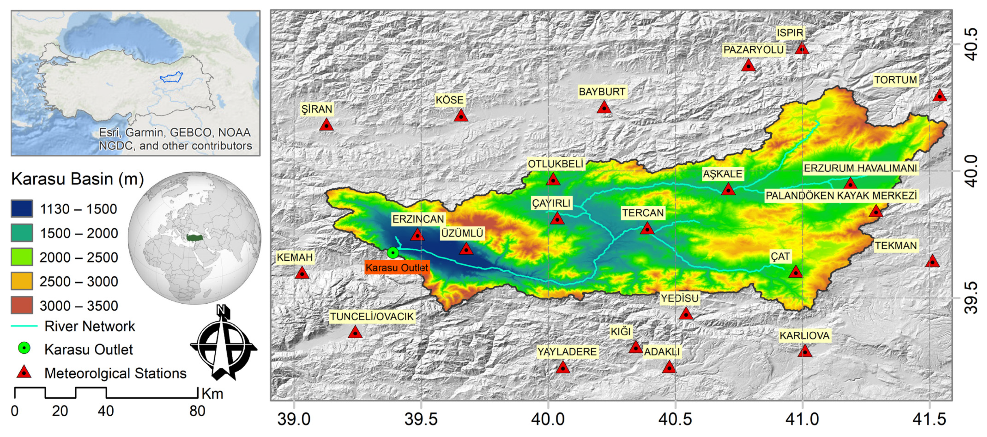
2.1. Study Area

The Karasu basin (38°58′ E to 41°39′ E and 39°23′ N to 40°25′ N) is defined as the study area controlled by Kemah (E21A019) hydrological station (Figure 1) located in the eastern part of Turkey. The basin has a drainage area of around 10,250 km² and elevation ranges from 1130 m to 3500 m. Considering the terrain complexity and mountainous climate regime, most precipitation occurs in the form of snow and is retained on the ground for almost half a year, contributing to streamflow when the temperatures increase. The Karasu basin is one of the major tributaries of the Euphrates River, known as the longest transboundary river in southwest Asia and being the largest river basin (127,300 km²) with a 17% total water potential in Turkey that embraces large man-made reservoirs used for irrigation, water supply, hydropower, and flood control purposes. Hence, evaluating the hydrologic response of different GPDs over an important headwater catchment is crucial for the optimal management of water resources.

2.2. Hydro-Meteorological Data

In this study, daily observed precipitation and temperature data from 23 ground-based stations (independent stations whose data are not shared and evaluated with worldwide research centers for bias correction of gauge corrected GPDs) are used to validate 13 selected GPDs in and around the Karasu basin. Moreover, daily streamflow data collected at the outlet of the basin is utilized to assess the hydrologic performance of GPDs. All the above-mentioned data are evaluated for five recent water years from October 2014 to September 2019.

In this context, the study uses daily based precipitation data obtained from 13 selected GPDs whose detailed information is presented in

Table 1. Properties of selected GPDs. Abbreviations in the data source represent; G, Gauge; S, Satellite; and R, Reanalysis. Abbreviation in the temporal coverage represent; NRT, Near Real-Time.

Dataset Name	Data Source(s)	Spatial Resolution	Spatial Coverage	Temporal Resolution	Temporal Coverage	Latency	References
CPCv1	G	0.50°	Global	Daily	1979–Present	1 day	[40]
MSWEPv2.8	G, S, R	0.10°	Global	3-hourly	1979–NRT	Few months	[41,42]
ERA5	R	0.25°	50° N/S	Hourly	1979-Present	3 months	[43]
CHIRPSv2.0	G, S, R	0.05°	L-50° N/S	Daily	1981–NRT	1 month	[44]
CHIRPv2.0	S, R	0.05°	L-50° N/S	Daily	1981–NRT	2 days	[44]
IMERGHHFv06	G, S	0.10°	60° N/S	30 min	2014–NRT	~3.5 months	[45]
IMERGHHEv06	S	0.10°	60° N/S	30 min	2014–NRT	4 h	[45]
IMERGHHLv06	S	0.10°	60° N/S	30 min	2014–NRT	14 h	[45]
TMPA-3B42v7	G, S	0.25°	50° N/S	3-hourly	2000–Present	3 months	[46]
TMPA-3B42RTv7	S	0.25°	50° N/S	3-hourly	1998–NRT	1 day	[46]
PERSIANN-CDR	G, S	0.25°	60° N/S	Daily	1983–2016	3 months	[47]
PERSIANN-CCS	S	0.04°	60° N/S	Hourly	2003–NRT	1 h	[48]
PERSIANN	S	0.25°	60° N/S	Hourly	2000–NRT	2 days	[49]

: Climate Prediction Center unified V1 (CPCv1), Multi-Source Weighted-Ensemble Precipitation (MSWEP) V2.8, European Centre for Medium-Range Weather Forecasts (ECMWF) reanalysis fifth-generation (ERA5), Climate Hazards group InfraRed Precipitation with Stations (CHIRPS) V2.0, Climate Hazards group InfraRed Precipitation (CHIRP) V2.0, Integrated Multi-satellitE Retrievals for GPM (IMERG) final run V06, Integrated Multi-satellitE Retrievals for GPM (IMERG) Early run V06, Integrated Multi-satellitE Retrievals for GPM (IMERG) late run V06, TRMM Multi-satellite Precipitation Analysis (TMPA) 3B42 V7, TRMM Multi-satellite Precipitation Analysis (TMPA) 3B42RT V7, Precipitation Estimation from Remotely Sensed Information using Artificial Neural Networks (PERSIANN) Climate Data Record (CDR), Precipitation Estimation from Remotely Sensed Information using Artificial Neural Networks (PERSIANN) Cloud Classification System (CCS), and Precipitation Estimation from Remotely Sensed Information using Artificial Neural Networks (PERSIANN).

Considering input and methodology, selected GPDs can be categorized into four different groups: (1) taking advantage of spatial information from ground-based gauge precipitation data (CPCv1); (2) utilizing reanalysis data from numerical weather prediction model outputs (ERA5); (3) using satellite Passive Microwave (PMW) and Infrared (IR) sensor data (IMERGHHEv06, IMERGHHLv06, TMPA-3B42RTv7, PERSIANN, and PERSIANN-CCS); and (4) multi-source merging precipitation datasets with gauge uncorrected (CHIRPv2.8) as well as gauge corrected products (MSWEPv2.8 and CHIRPSv2.0, IMERGHHFv06, TMPA-3B42v7, and PERSIANN-CDR). Furthermore, gauge corrected multi-source merging precipitation datasets use gauge-based precipitation measurements from various sources having different spatial and temporal resolutions. For example, TMPA-3B42v7 and IMERGHHFv06 use monthly Global Precipitation Climatology Centre (GPCC) with 1° spatial resolution [45,46] and PERSIANN-CDR utilizes monthly Global Precipitation Climatology Project (GPCP) datasets with a 2.5° spatial resolution [47]. Moreover, CHIRPSv2.0 includes pentadal precipitation estimates from the Climate Hazards group Precipitation climatology (CHPclim) datasets and daily precipitation data from other national meteorological agencies and private streams [44]. MSWEPv2.8 includes WorldClim 2 datasets with 1 km spatial resolution and use monthly GPCC, Global Historical Climatology Network-Daily (GHCN-D), Summary of the Day (GSOD), and other gauge observations [42]. GPDs can also be differentiated by their spatial and temporal resolution/coverage. For example, PERSIANN-CCS has the highest spatial resolution (0.04°) with hourly precipitation data existing from 2003 to near real-time while covering an area of 60° N/S. On the other hand, CPCv1 has a coarser spatial resolution (0.50°) with global coverage exhibiting daily precipitation from 1997 to the present. Moreover, the time in which the dataset is released for public use is an important factor for hydro-climatological studies such as flood forecasting and early warnings. For example, IMERGHHEv06 is released after 4 h of real-time while its final research product (IMERGHHFv06) is released for public use after 3.5 months.

2.3. Methodology

The Kling-Gupta Efficiency [50,51] objective function is used to assess the performance of GPDs. Kling-Gupta Efficiency (KGE) has three components, the Pearson correlation coefficient (r) presents the temporal dynamics of precipitation, bias (β), and the variability ratio (γ), determine the volume distribution of precipitation. The Nash-Sutcliffe Efficiency (NSE) and KGE are utilized to evaluate the strength of 13 GPDs for reproducing streamflow time series. Moreover, the Hanssen-Kuiper (HK) Score is used to show the strength of GPD distinguishing between occurrences and non-occurrences of a certain event. Finally, the probability density function (PDF) is exploited to classify the rainfall intensity occurrences of GPDs and observed gauge precipitation [52,53].

Table 2. Properties of performance indices for evaluation of GPDs.

Performance Indicator	Mathematical Statement	Explanation
Kling-Gupta Efficiency and its components	$KGE=1-[{\left(r-1\right)}^2+{\left(\beta -1\right)}^2+{\left(\gamma -1\right)}^2{]}^{0.5}$ $r=\frac{1}{n}{\displaystyle {\displaystyle \sum }_1^n}\left(o_n-{\mu }_0\right)\left(s_n-{\mu }_s\right){/(\delta }_o{\times \delta }_s),$ $\beta =\frac{{\mu }_s}{{\mu }_o}{,\gamma =(\delta }_s{\times \mu }_o{)/(\mu }_s{\times \delta }_o)$	r (Pearson correlation coefficient), β (Bias) is the ratio of estimated and observed mean, γ (Variability Ratio) is the ratio of estimated and observed coefficients of variation, µ and δ are the distribution mean and standard deviation where s and o indicate estimated and observed. M (Miss); when the observed precipitation is not detected. F (False); when the precipitation is detected but not observed, H (Hit); when the observed precipitation is correctly detected, CN (Correct Negative); a no precipitation event is detected. n is the sample size of the observed or calculated streamflow. $Q_i^o$ and $Q_i^s$present the observed and simulated streamflow, $\overline{Q_i^o}$ present the mean observed streamflow.
Hanssen-Kuiper	$HK=\frac{\left(H\times CN\right)-(F\times M)}{\left(H+M\right)(F+CN)}$
Nash-Sutcliffe Efficiency	$NSE=1-\frac{{{\displaystyle \sum }}_{i=1}^n{{(Q}_i^s{-Q}_i^o)}^2}{{{\displaystyle \sum }}_{i=1}^n{{(Q}_i^o-\overline{Q_i^o})}^2}$

shows the properties of selected evaluation metrics whereby the optimal value is unity for each of them.

The daily-based precipitation events from gauge and GPDs are discretized into five thresholds considering World Meteorological Organization [54] standard for rainfall intensity classification later modified by Zambrano-Bigiarini [55]. The five precipitation thresholds considered are no-precipitation (less than 1 mm/day), light precipitation (1–5 mm/day), moderate precipitation (5–20 mm/day), heavy precipitation (20–40 mm/day), and violent precipitation (more than 40 mm/day). This categorization is important for hydrological studies whereby different intensity classes may present a distinct hydrologic response over the basin. A point to grid approach is selected for comparison of GPDs with gauge precipitation data where the value of each grid box at the station location is extracted by linear interpolation [56]. Finally, based on the temporal availability of observed and GPDs, the evaluation period is selected from October 2014 to September 2019.

The conceptual TUW hydrological model successfully tested in several studies [57,58,59,60,61,62] is utilized in this work. The TUW model is developed based on the similar structure of the widely recognized Hydrologiska Byråns Vattenbalansavdelning (HBV) [63,64] model and operates on a daily time step. TUW model inputs are total precipitation (mm), mean air temperature (°C), and potential evapotranspiration (mm) and include 15 model parameters (

Table 3. TUW model parameter properties.

No	ID	Description	Units	Process	Range
1	SCF	Snow correction factor	-	Snow	0.9–1.5
2	DDF	Degree-day factor	mm/°C/day	Snow	0.0–5.0
3	Tr	Temperature threshold above which precip. is rain	°C	Snow	1.0–3.0
4	Ts	Temperature threshold below which precip. is snow	°C	Snow	−3.0–1.0
5	Tm	Temperature threshold above which melt starts	°C	Snow	−2.0–2.0
6	LPrat	Parameter related to the limit for potential evaporation	-	Soil Moisture	0.0–1.0
7	FC	Field capacity	mm	Soil Moisture	0.0–600
8	BETA	Non-linear parameter for runoff production	-	Soil Moisture	0.0–20
9	cperc	Constant percolation rate	mm/day	Runoff	0.0–8.0
10	k0	Storage coefficient for very fast response	day	Runoff	0.0–2.0
11	k1	Storage coefficient for fast response	day	Runoff	2.0–30
12	k2	Storage coefficient for slow response	day	Runoff	30–250
13	lsuz	Threshold storage state	mm	Runoff	1.0–100
14	bmax	Maximum base at low flows	day	Runoff	0.0–30
15	croute	Free scaling parameter	day2/mm	Runoff	0.0–50

) to calibrate snow, soil moisture, and runoff routines. The hydroPSO R package, which includes the particle swarm global optimization algorithm [65,66], is used to calibrate the TUW model parameters.

Generally, two types of hydrologic simulation scenarios are widely used for the hydrologic utility of GPDs depending on the level of information provided: (a) model parameters are fitted according to simulated and observed streamflow time series using observed precipitation data as input and afterward the observed precipitation is replaced by GPDs for validation. This method is more efficient for gauged basins. In the second type, (b) model parameters are calibrated/validated with streamflow data using each GPD as a model input independently. This method is recommended for ungauged basins where only observed streamflow and GPDs are available [4,67]. Hence, in this study, both schemes are considered for the hydrologic response of the basin based on observed and GPDs input.

3. Result and Discussion

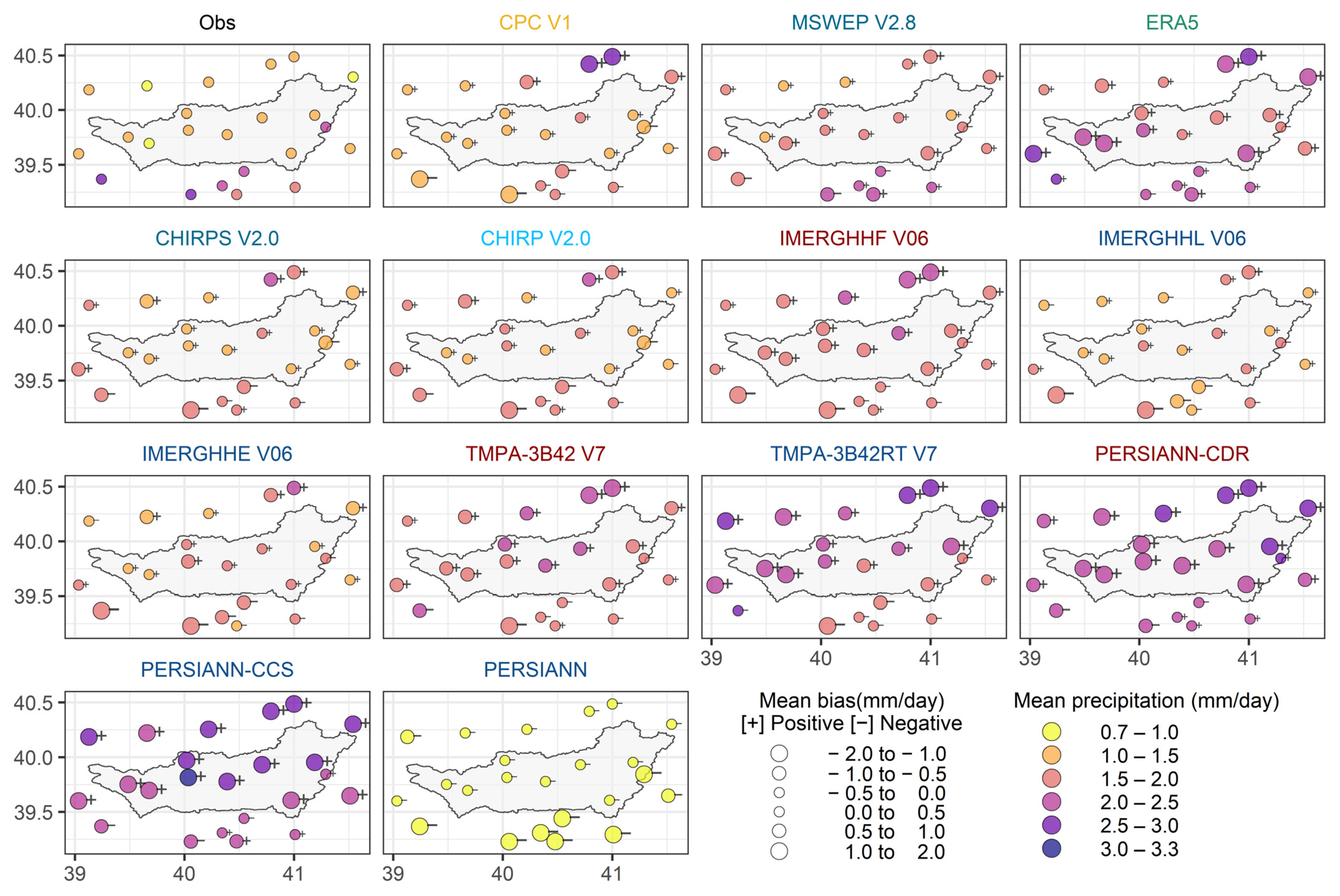
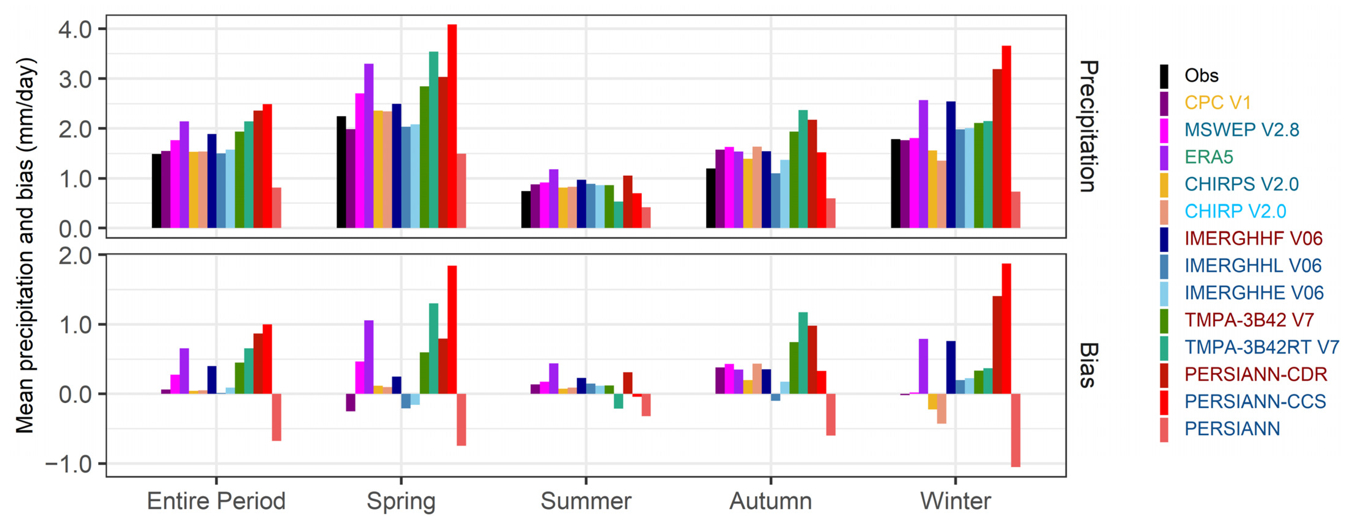
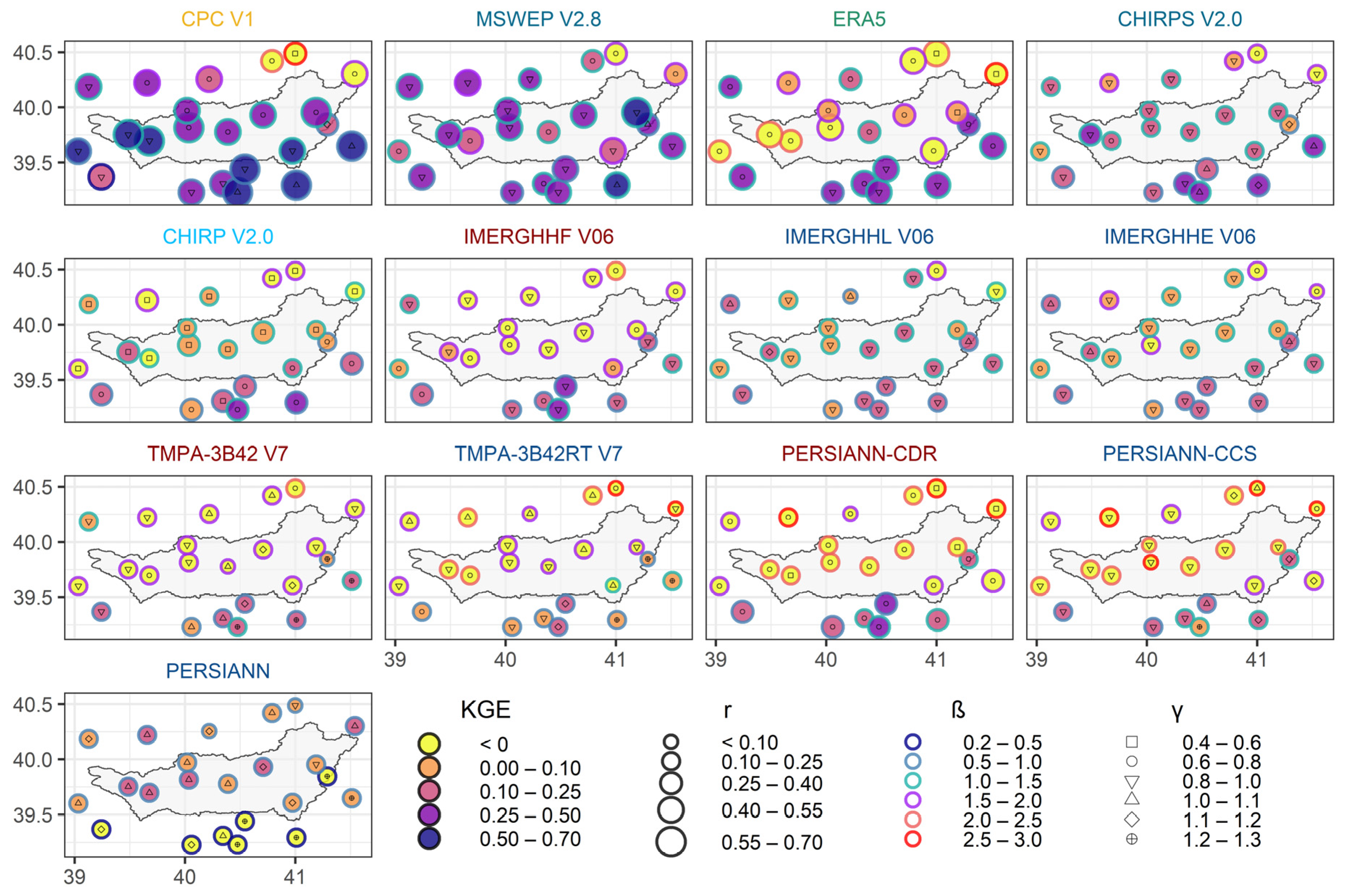
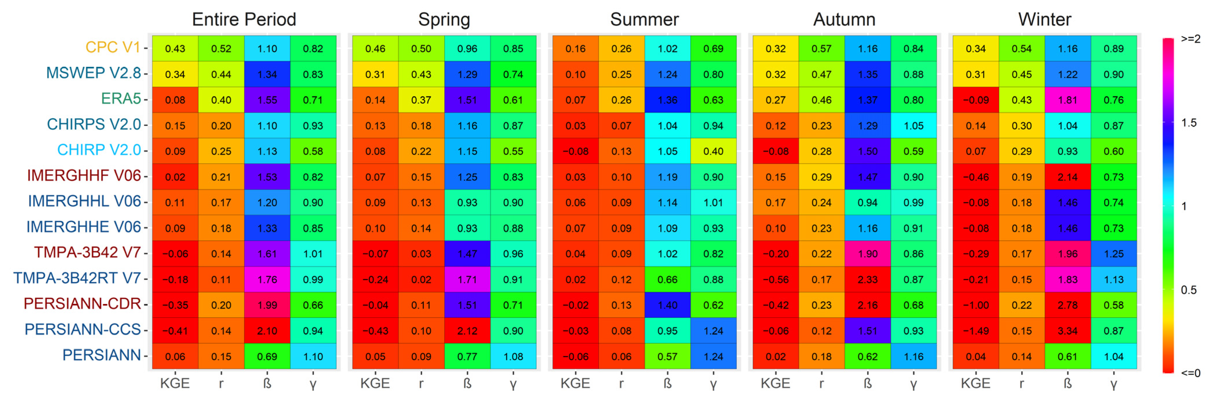
3.1. Spatial and Temporal Evaluation of Daily Precipitation

Figure 2 shows the spatial distribution of the mean daily precipitation derived from observed gauges and 13 GPDs, including their bias, at the corresponding ground station location for the selected period (2015–2019). Considering the observed data, the mean daily precipitation increases from the north (1–1.5 mm) to the south (2.5–3 mm) of the basin. CPCv1, the only selected GPD which is developed based on information collected from ground station networks, is able to reproduce mean daily precipitation of around 1–2 mm/day inside the basin. However, this dataset overestimates precipitation in the northeast and underestimates in the southwest part of the basin with a varying mean daily precipitation bias from −0.5 to 0.5 mm. ERA5 presents higher mean daily precipitation (1.5–2.5 mm) compared to the observed precipitation with overestimating bias in and around the area of study. Among the GPDs that provide information by combining different sources, both CHIRPSv2.0 and CHIRPv2.0 reproduce the mean daily precipitation quite well (1–1.5 mm), especially within the basin, and their bias varies from 0 to 0.5 mm, while MSWEPv2.8 estimates higher precipitation (1.5–2 mm) and a slightly larger bias.

Overall, GPDs that combine only ground and satellite data (G, S), seem to map mean daily precipitation poorly compared to other multi-source products. IMERGHHFv06 is able to represent slightly better mean daily precipitation (1.5–2 mm) compared to TMPA3B42v7 (1.5–2.5 mm) while PERSIANN-CDR presents higher daily precipitation (2–3 mm) and shows precipitation bias of 1–2 mm comparatively. Among GPDs which only use satellite data, IMERGHHEv06 and IMERGHHLv06 are able to reproduce mean daily precipitation (1–2 mm) well compared to adjusted (IMERGHHFv06) and other satellite-based GPDs such as TMPA-3B42RTv7 (1.5 to 2.5 mm). In the same way, PERSIANN-CCS is one of the GPDs which presents higher mean daily precipitation (2–3 mm) and a precipitation bias close to PERSIANN-CDR (1–2 mm), while PERSIANN always shows mean daily precipitation less than 1 mm and its bias increasing from the north (−0.5–0 mm) to the south (−1 mm to −2 mm).

Figure 3 shows the mean daily precipitation and its estimated bias for the selected GPDs at the regional scale considering the entire period and four seasons (Spring, Summer, Autumn, and Winter). According to observed mean daily precipitation, the region receives more precipitation during the spring (2.24 mm) followed by winter (1.78 mm), while the summer (0.74 mm) and autumn (1.2 mm) seasons show less precipitation with a 1.5 mm mean daily precipitation estimated over the Karasu basin for the entire period. CPCv1 presents mean precipitation that is close to the observed for the entire period and all seasons where the estimated mean daily precipitation bias does not exceed ±0.3 mm. Among multi-source merging GPDs, both CHIRPv2.0 and CHIRPSv2.0 reproduce mean daily precipitation well and only underestimate precipitation during the winter season (bias; −0.22 mm for CHIRPSv2.0 and −0.43 mm for CHIRPv2.0). MSWEPv2.8 gives values close to the observed during winter and overestimates precipitation for the rest of the seasons and the entire period, indicating high overestimation for the spring season (0.5 mm). ERA5 estimates more precipitation compared to observed during the spring season (3.3 mm, bias; 1.1 mm) and is able to reproduce autumn precipitation (1.5 mm, bias; 0.3 mm) well enough. Among GPDs which combine only ground and satellite data (G, S), IMERGHHFv06 produces good results on mean daily precipitation for the entire period (1.8 mm), spring (2 mm), and autumn (1.5 mm) compared to TMPA-3B42v7 which performs better during the summer (0.8 mm) and winter (2.1 mm) seasons. PERSIANN-CDR always overestimates mean daily precipitation and it shows a higher bias during winter (bias; 1.8 mm), comparatively. Among satellite-based GPDs, both IMERGHHEv06 and IMERGHHLv06 reproduce mean daily precipitation close to observed while TMPA-3B42RTv7 and PERSIANN-CCS overestimate and PERSIANN significantly underestimates considering the entire period and four seasons.

Figure 4 displays the daily precipitation scatter plots of 13 GPDs against observed data and mean daily precipitation over the Karasu basin for each year of the study period. Daily precipitation events from observed and 13 GPDs mostly concentrate between 0–50 mm. However, CPCv1 shows the highest correlation (0.52) to the observed precipitation compared to other GPDs and TMPA-3B42RTv7 presents the lowest correlation (0.10) for daily precipitation values. MSWEPv2.8 presents the second-best overall correlation (0.44) having the better of the other multi-sources merging GPDs (CHIPRv2.0 and CHIRPSv2.0) followed by ERA5 (0.39). Among GPDs which combine only ground and satellite data, IMERGHHFv06 presents a high correlation (0.21) compared to PERSIANN-CDR (0.19) and TMPA3b42v07 (0.14). IMERGHHEv06 shows a better correlation (0.18) while the other satellite-based GPD (IMERGHHLv07, TMPA-3B42RTv7, PERSIANN-CCS, and PERSIANN) correlations to the observed precipitation are not higher than 0.17. The Karasu basin received different amounts of daily mean precipitation from 2015 to 2019 water years, 2017 having the least amount. CPCv1 presents a close precipitation estimate to observed whereby PERSIANN-CCS and PERSIANN-CDR indicate significant overestimates along with PERSIANN displaying noteworthy undervalues.

3.2. Consistency of GPDs over Time and Space

Figure 5 maps the spatial distribution of the Kling-Gupta Efficiency (KGE), along with its correlation (r), bias (β), and variability ratio (γ) components of daily precipitation at 23 station locations for the entire period. As expected, the best performance (KGE; 0.5–0.7, r; 0.55–0.70) is obtained by CPCv1 which is the only dataset with temporal variation entirely depending on ground data. Some discrepancies are detected over the northeast regions resulting in low correlation (0.25–0.4) and variability ratio (0.4–0.8) with a high bias (2–3). Among multi-source merging GPDs, MSWEPv2.8 shows close performance (KGE; 0.25–0.7, r; 0.25–0.7) to CPCv1 followed by CHIRPSv2.0 (KGE; 0.1–0.5, r; 0.1–0.25), indicating the importance of aggregating daily gauge data [41,42,44]. However, CHIRPSv2.0 overestimates bias (bias; 1–1.5) and its variability ratio varies from 0.8 to 1.2 while CHIRPv2.0 shows poor performance compared to MSWEPv2.8 and CHIPRSv2.0. ERA5 performs better in the southern areas (KGE; 02.5–0.50) while within the basin and in the northern areas its performance is much dispersed. All GPDs with satellite and gauge combination have a low performance inside the basin and in the northern part (KGE; <0) but perform better in the southern areas (KGE; 0.1–0.25). IMERGHHLv06 and IMERGHHEv06 show a higher performance compared to its gauge corrected (IMERGHHFv06) dataset and other satellite-based GPDs, although these two datasets show a close performance to CHIRPSv2.0 and CHIRPv2.0. PERSIANN, being another satellite-based GPD, performs better than PERSIANN-CCS and PERSIANN-CDR. Unlike other GPDs, PERSIANN shows high performance in the northern area yet performs poorly in the southern part. TMPA-3B42RTv7 performs poorly compared to other satellite-based GPDs but presents a close relation to its gauge corrected (TMPA-3B42v7) dataset.

Figure 6 shows the median Kling-Gupta Efficiency (KGE) and its three components (correlation, bias, and variability ratio) for the entire period, all four seasons (spring, summer, autumn, and winter), and considers daily precipitation. CPCv1 shows the best performance for the entire period and four seasons, compared to other GPDs, with a higher spring (median KGE; 0.46) and a lower summer (median KGE; 0.16) result. Among multi-source merging GPDs, MSWEPv2.8 performs better (median KGE; 0.34) followed by CHIRPSv2.0 (0.15) and CHIRPv2.0 (0.09) for the entire period.

The best performance for ERA5 comes within the autumn season (median KGE; 0.27) while showing lower results (median KGE; −0.09) during winter. This diverse performance of ERA5 over time and space may be attributed to the limited numerical weather prediction model utilized to demonstrate small-scale convective cells, in line with previous studies [68,69]. All GPDs which combine only gauge and satellite data, give poor results. While IMERGHHFv06 performs slightly better during spring and autumn, TMPA-3B42v7 can only present a positive KGE in summer. This indicates that the successor (IMERGHHFv06) shows a slightly higher performance compared to its predecessors (TMPA-3B42v7) which is consistent with previous evaluations over Turkey [32] and may be related to product algorithm improvements [45]. PERSIANN-CDR performs poorly in all four seasons. This low performance of satellite-gauge combination GPDs could firstly be attributed to the satellite-based algorithm and subsequently to the gauge correction procedure. As mentioned before in Section 2.2, gauge correction is applied from different sources using a different number of gauges, hence it is more important to know how much information from gauge data is delivered by each gauge corrected GPD within the complex topographic region. IMERGHHEv06 and IMERGHHLv06 show a better outcome compared to other satellite-based GPDs for the entire period and four seasons. PERSIANN performs better than its gauge corrected dataset (PERSIANN-CDR) and PERSIANN-CCS overall. Among all GPDs, PERSIANN-CCS shows the overall highest bias and PERSIANN giving the lowest. The highest observed overestimate is given by PERSIANN-CCS in winter (3.34) while the highest underestimate is detected by PERSIANN in summer (0.57). Hence, GPDs exclusively based on satellite (PMW or IR) show low performance over complex topography and snow dominant regions, consistent with earlier studies concerned with GPD validations [70,71,72].

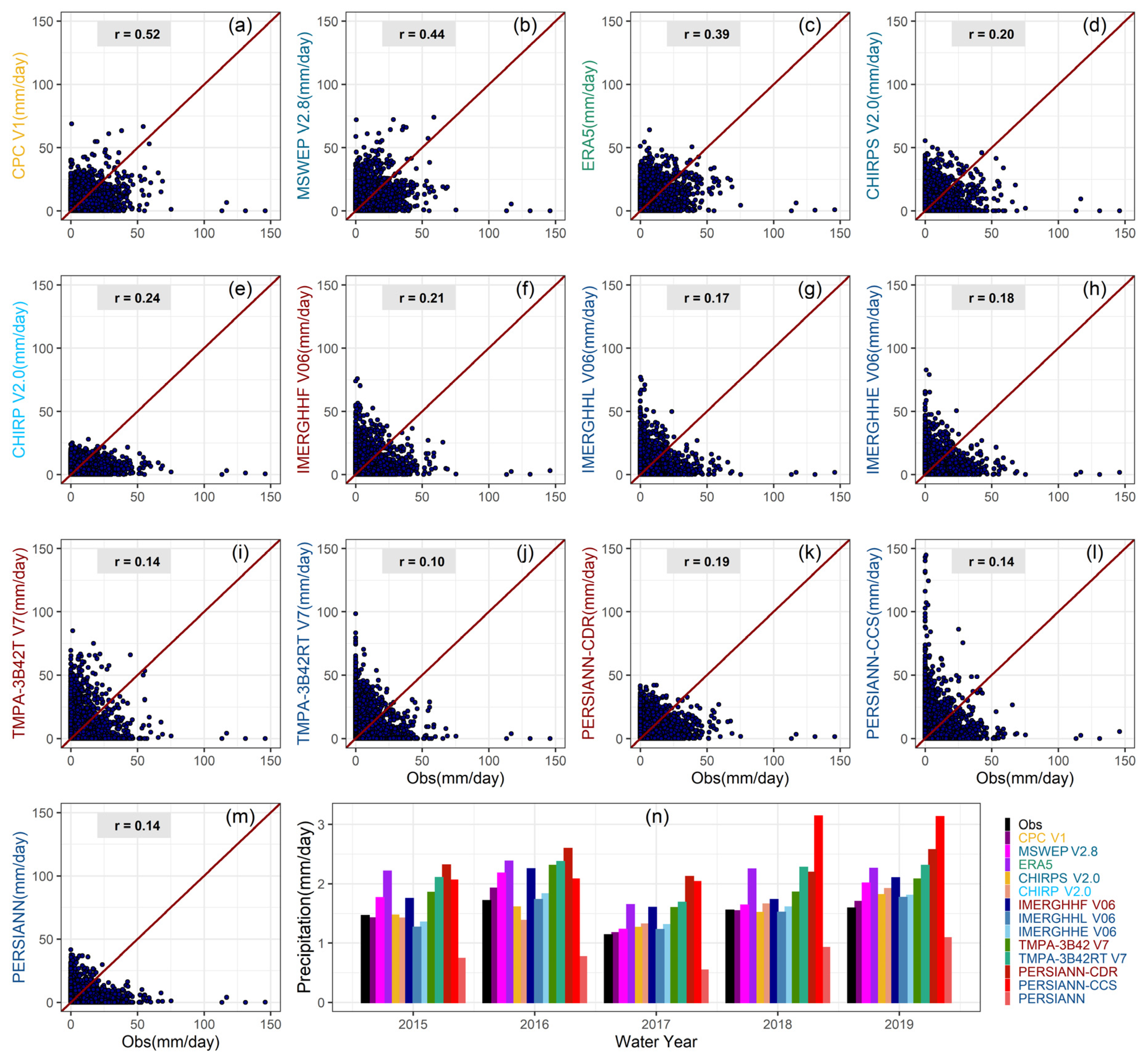
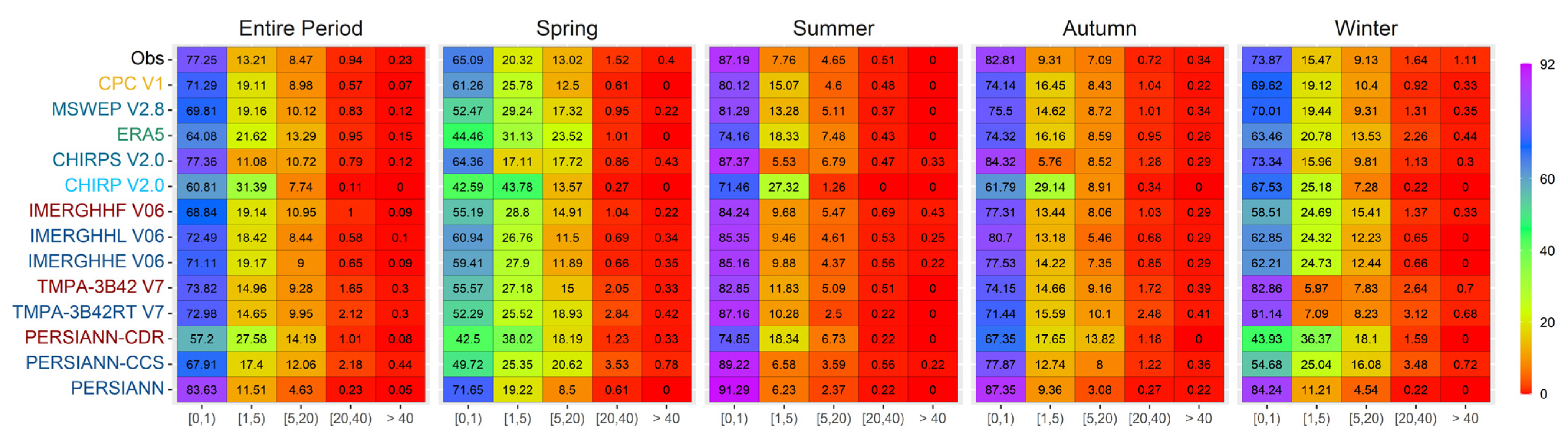
3.3. GPD Precipitation Intensity Comparison

Figure 7 shows the result of precipitation frequencies of various intensities derived from gauge precipitation and 13 GPDs during the entire period and four seasons. Based on the observed data, 77% of precipitation events occur in the range of 0–1 mm/day for the entire period while this amount decreases for spring and winter precipitation and shows more frequency during summer and autumn. Furthermore, as expected, the frequency of precipitation events decreases as the intensity of precipitation increases. GPDs show varying frequencies of precipitation intensities that are especially noticeable during the spring season. PERSIANN shows more precipitation intensities for 0–1 mm/day compared to the observed and presents less frequency for light precipitation (1–5 mm/day) events during the entire period and all seasons. Among multi-source merging GPDs, CHIRPSv2.0 presents precipitation frequencies close to the observed intensity of 0–1 mm/day while CHIRPv2.0 and MSWEPv2.8 overestimate light precipitation. In the same way, PERSIANN-CDR significantly overestimates light precipitation (1–5 mm/day) and underestimates 0–1 mm/day intensities compared to IMERGHHFv06 and TMPA-3B42v7 for the entire period and four seasons. PERSIANN is the only satellite-based GPD that overestimates precipitation 0–1 mm/day and underestimates other precipitation events (light, moderate, heavy, and violent precipitation). IMERGHHEv06 and IMERGHHLv06 show close frequencies to the observed for different intensities during the entire period and four seasons. TMPA-3B42RTv7 shows similar results as its gauge corrected (TMPA-3B42v7) dataset.

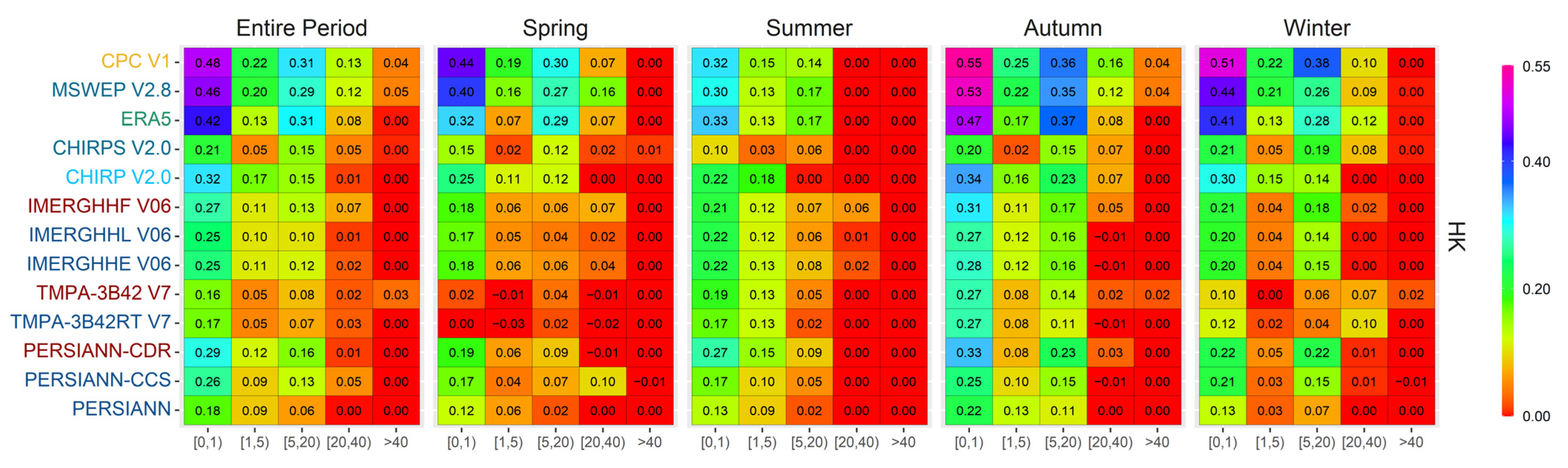
3.4. Evaluation of GPD Detectability

Figure 8 shows the detectability strength of 13 GPDs for five different daily precipitation groups considering the entire period and four seasons expressed in the form of the Hanssen-Kuiper (HK) score. Overall, GPDs show higher detectability during autumn and lower during summer; additionally, the detection strength of GPDs decreases as the precipitation intensity increases which is generally the case in literature. This can be attributed to the classification of several intensity classes which makes it hard to differentiate among them instead of a simple rain/no rain scenario. This division gets even more problematic when the occurrence probability of a certain event is seen much more rarely compared to other classes (heavy and violent intensities) as can be followed from Figure 7. Hence, detecting a rarely occurring very intense precipitation event has a weaker performance when assessed against a more frequently occurring light storm.

From the results, CPCv1 shows the highest detectability for intensity less than 1 mm/day and light precipitation (1–5 mm/day), followed by MSWEPv2.8 and ERA5. CHIRPv2.0 shows better detectability for precipitation less than 1 mm/day, light and moderate precipitation compared to CHIRPSv2.0 while CHIRPSv2.0 presents slightly better results for heavy and violent precipitation. IMERGHH datasets show similar detectability values to each other considering different precipitation groups while TMPA datasets portray lower detectability values compared to IMERGHH products. PERSIANN-CDR performs better when evaluated against PERSIANN-CCS and PERSIANN.

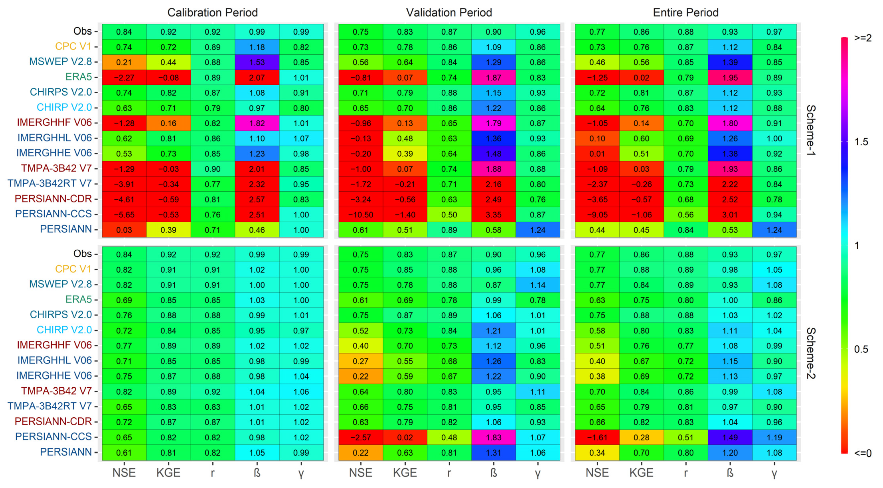
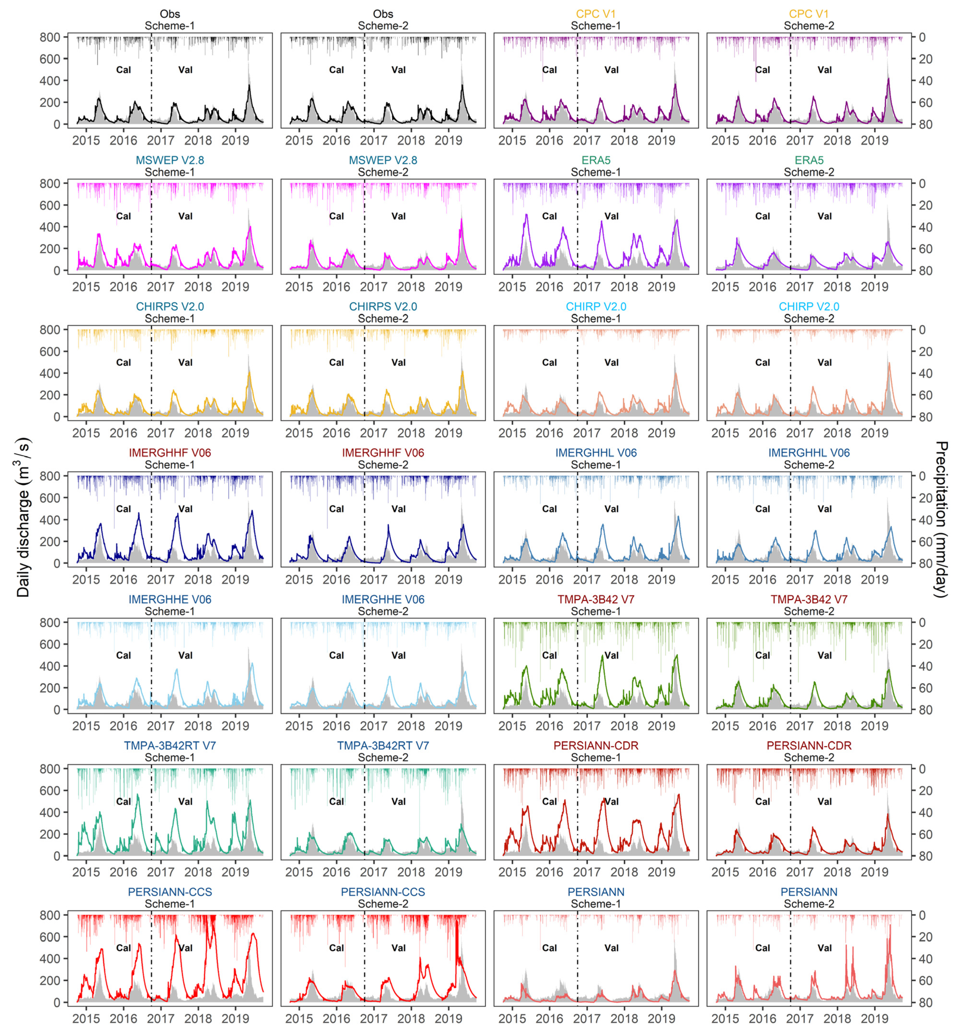
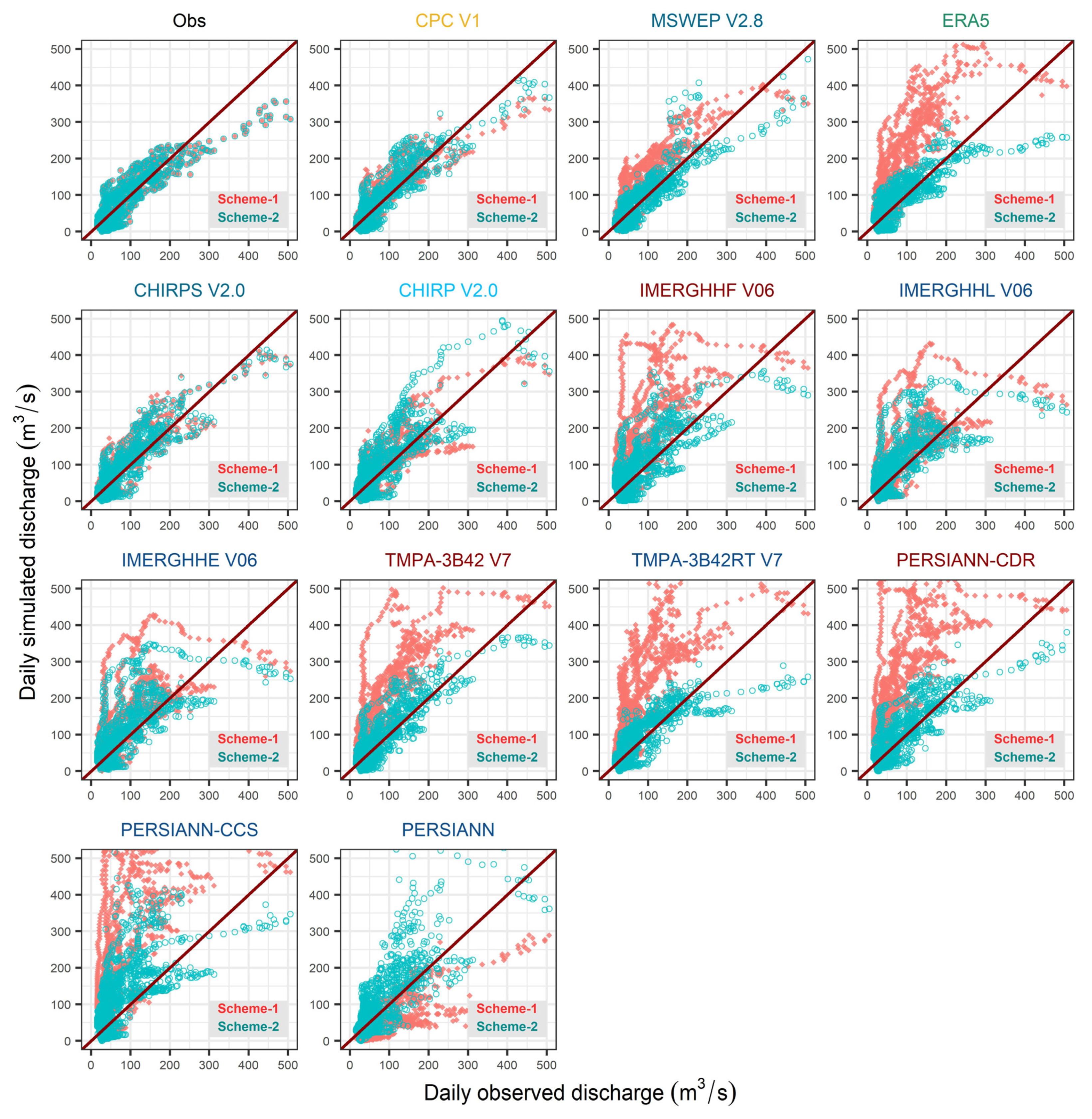
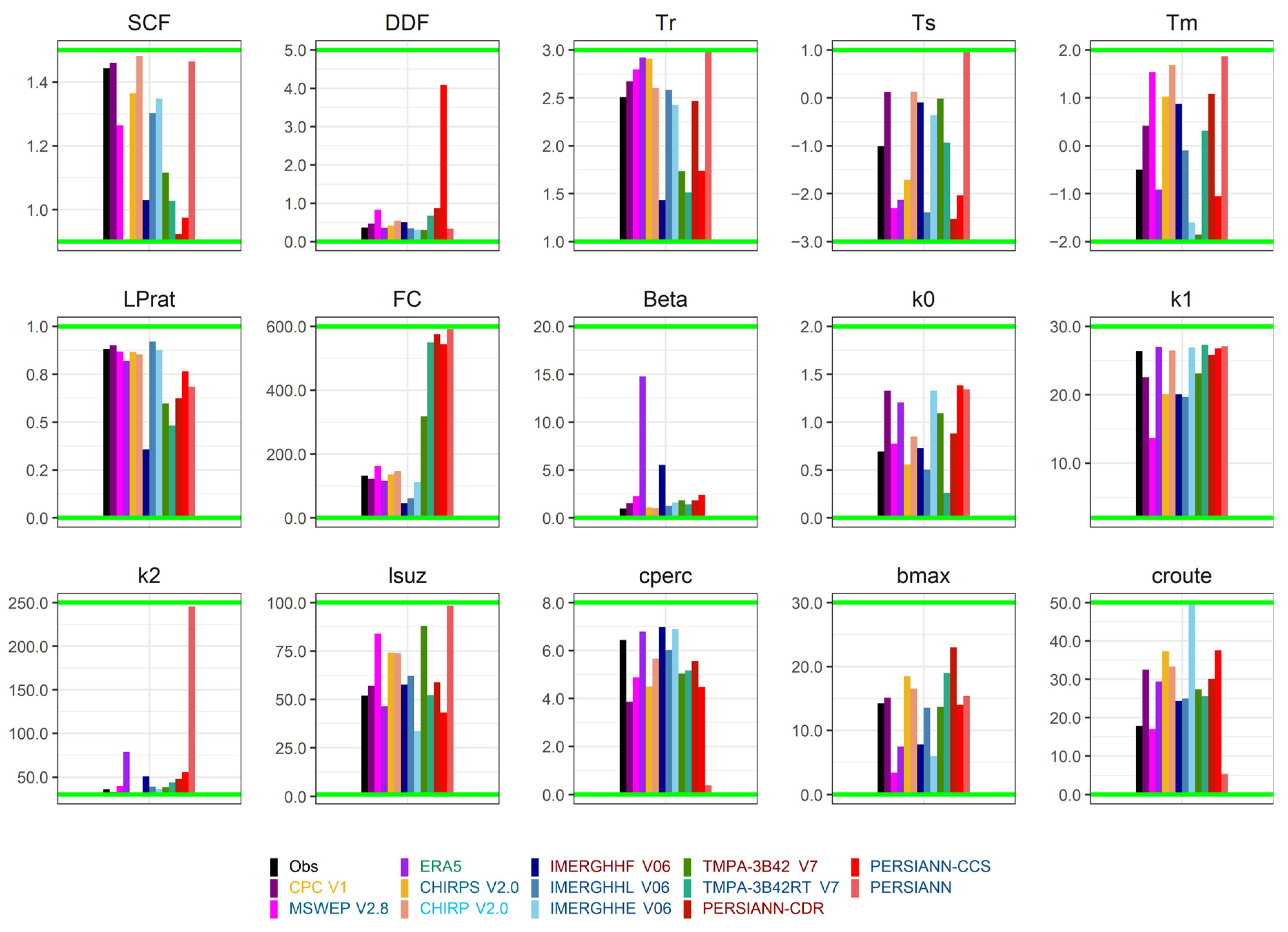
3.5. Hydrologic Evaluation of GPDs

The TUW model is utilized to simulate streamflow at the Karasu basin outlet from 2015 to 2019 using observed precipitation and 13 GPDs in two steps. Firstly, model parameters are calibrated by observed data and then replaced by each GPD (Scheme-1). Afterward, model parameters are calibrated based on observed data and each GPD individually (Scheme-2). Figure 9 displays the hydrographs at the basin outlet for different precipitation input products considering the two schemes. In all cases, the model is calibrated for two waters years (October 2014–September 2016) and validated for three water years (October 2016–September 2019).

Figure 10 depicts the scatter plot of simulated daily streamflow against the observed discharge obtained from in situ precipitation and selected GPDs at the basin outlet considering the two schemes. Generally, GPDs show a higher streamflow amount in Scheme-1 compared to Scheme-2. However, CHIRPSv2.0 displays quite comparable discharge values when the model parameters are calibrated either by observed precipitation (Scheme-1) or GPD itself (Scheme-2). For high flows, PERSIANN underestimates streamflow more in Scheme-1 than Scheme-2. ERA5 shows distinct streamflow differences for the two schemes and its reproducibility improves when the model parameters are calibrated by ERA5 (Scheme-2). MSWEPv2.8 exhibits close streamflow amounts for both schemes, but shows slightly more discharge in Scheme-1. Both IMERGHHEv06 and IMERGHHLv06 demonstrate less variation of streamflow compared to IMERGHHFv06. The rest of the GPDs indicate better streamflow reproducibility for Scheme-2 than Scheme-1.

The nonlinearity of simulated streamflow can be related to the high bias which is noted in the direct comparison of GPDs with observed precipitation (Section 3.2 and Figure 5 and Figure 6). Moreover, in Scheme-1, model parameters are calibrated by observed precipitation only, which is not an optimal parameter set for GPDs. This may be the reason for high degradation (overestimates) in GPD streamflow prediction during the calibration/validation period (especially for ERA5, IMERGHH datasets, TMPA datasets, PERSIANN-CDR, and PERSIANN-CCS). Furthermore, it should be kept in mind that for Scheme-2 modeling, precipitation values are taken from GPDs while PET and temperature values are still a part of observed meteorological forcing in the model.

Figure 11 shows the Kling-Gupta Efficiency (KGE) with its three components (correlation, bias, and variability ratio) and Nash–Sutcliffe Efficiency (NSE) streamflow modeling results for the two schemes considering calibration, validation, and entire periods. When the model is forced to simulate streamflow with observed gauge data, it reproduces quite high KGE (0.92) and NSE (0.84) with almost no bias and variability ratio during the calibration period. The model is able to keep the good performance for the validation period with KGE (0.83) and NSE (0.75) scores. In Scheme-1, CPCv1 performs close to the observed results for daily streamflow simulation with a slight overestimation in bias and underestimation in variability ratio for all phases. Among multi-sources merging GPDs, both CHIRPv2.0 and CHIRPSv2.0 display a good performance for the calibration and validation periods as compared to MSWEPv2.8 which, interestingly, presents better results for its validation stage than calibration. Moreover, IMERGHHFv06, TMPA-3B42v7, PERSIANN-CDR, and ERA5 perform poorly in simulating the streamflow for Scheme-1. Among satellite-based GPDs, both IMERGHHEv06 and IMERGHHLv06 show positive performance for the calibration period with their performance decreasing (with negative NSE) for validation and the entire period. TMPA-3b42RTv7 and PERSIANN-CCS perform poorly in simulating the streamflow for all periods and show negative KGE and NSE. The PERSIANN dataset shows varying performance compared to other GPDs and underestimates bias and overestimates the variability ratio. When the model parameters are calibrated based on each GPD individually (Scheme-2), all GPDs simulate streamflow with high performance for the calibration period. MSWEPv2.8 shows close reproducibility of streamflow to CPCv1 and observed discharge for calibration, validation, and the entire period. Comparatively, PERSIANN-CCS shows high KGE (0.82) and NSE (0.65) during the calibration period but its reproducibility for streamflow generation is poor for validation and the entire period. Among all GPDs, CHIRPv2.0 and PERSIANN behave differently in Scheme-2. Both simulate streamflow well for the calibration phase while their performance decreases during validation and the entire period as compared to Scheme-1. PERSIANN-CCS significantly overestimates bias in both schemes. Overall, the TUW model shows good performance over snow dominant catchments as noted in the literature, and the relatively shorter time span for model calibration is one of the reasons for higher KGE.

Figure 12 presents the TUW model calibrated parameter values based on the observed data and 13 GPDs. PERSIANN-CCS shows quite a different DDF compared to other datasets. In the same way, ERA5 shows a high Beta, and PERSIANN displays a high K2 value. Additionally, TMPA and PERSIANN datasets show high FC compared to the rest of the GPDs. Further uncertainties arising from meteorological forcing and hydrological models may surely have an effect on streamflow simulations, but a detailed sensitivity/uncertainty analysis is not considered within the scope of this study.

4. Conclusions

In this study, the spatio-temporal consistency and hydrologic utility of 13 GPDs are evaluated over the mountainous Karasu basin from the 2015 to 2019 water years considering the observed daily precipitation from 23 meteorological stations in a daily time scale. The Kling-Gupta Efficiency (KGE) and Nash-Sutcliffe Efficiency (NSE) are considered to evaluate the spatial, temporal, and hydrologic response of the basin for different GPDs. Moreover, the Hanssen-Kuiper (HK) score is used to quantify the detectability strength of GPDs while the precipitation frequency for different precipitation intensities is assessed by the Probability Density Function (PDF). Finally, the rainfall-runoff modeling is conducted using the TUW model within two schemes. The major conclusions are itemized as follows:

• CPCv1 gathers information from ground station networks and displays a high performance for the rainfall distribution over time and space. This dataset also presents better detectability in terms of precipitation intensity and demonstrates valuable results when used in streamflow simulations.
• Among multi-source merging datasets, MSWEPv2.8 shows close performance to CPCv1 followed by CHIRPSv2.0 and CHIRPv2.0 for direct gauge comparison. CHIRPSv2.0 and CHIRPv2.0 outperform MSWEPv2.8 in accurately simulating streamflow especially in Scheme-1, but not in Scheme-2. GPDs which only use gauge and satellite data such as IMERGHHFv06, TMPA-3B42v7, and PERSIANN-CDR perform poorly in capturing precipitation intensities and show low reproducibility for streamflow generation in Scheme-1.
• Within satellite-based GPDs, IMERGHHEv06 and IMERGHHLv06 are able to perform better compared to other satellite-based products. While TMPA-3B42RTv7 and PERSIANN-CCS show low performance at all stages, PERSIANN generally underestimates precipitation. ERA5 shows slightly good performance both in spatial and temporal validation when compared to satellite-based GPDs and displays similar results for streamflow prediction in Scheme-2.
• Some satellite-based GPDs are becoming available with high spatial resolution and short time lag (latency) which is very important for real-time operation, but the existing bias limits their reliability for hydro-meteorological studies. As an example, PERSIANN-CCS is available after a one-hour time lag with 0.04° spatial resolution while its performance is not very high. On the other hand, IMERGHHLv06 presents precipitation after 14 h with a coarser spatial resolution (0.1°) compared to PERSIANN-CCS and is more reliable among selected satellite-based GPDs. Furthermore, when satellite-based GPDs are merged with other sources such as reanalysis and/or ground observation data, they become more accurate. For example, MSWEPv2.8 and CHIRPSv2.0 are the most reliable GPDs over the Karasu basin, but they have longer time lags varying from one month to a few months. It can be concluded that there are GPDs available for a near-real-time study and as product merging from different sources is implemented, increasing latency, the reliability of the new product seems to increase.
• Overall, most of the selected 13 GPDs have a low performance over time and space in detecting daily precipitation, but some of them can simulate streamflow quite accurately (Scheme-1). Furthermore, it is detected that GPDs demonstrate better reproducibility of streamflow when the model parameters are calibrated individually for each dataset (Scheme-2).

This study confirms the outperformance of CPCv1, MSWEPv2.8, and CHIRP(S)v2.0 products over other selected GPDs in the Karasu river basin located in the mountainous eastern part of Turkey. The results also indicate that GPDs making use of ground information in their retrospective algorithms may not always be able to attain reliable precipitation estimates. The information source, correction time window, and the number of gauges utilized are the important factors that considerably affect the final product’s reliability. Some near-real-time products (such as IMERGHHL(E)v06) show promising performance for short time lag availability. However, they still seem to be far off from being used in reliable streamflow simulations for early warning systems. Therefore, a pre/post-biased adjustment of satellite-based GPDs is recommended with possible high spatial and temporal resolution ground information. In addition, Scheme-2 hydrological modeling is recommended for ungauged basins where the calibration procedure uses GPD, ground temperature, and PET values. Since all model forcings will have their influence on optimal model parameters, it would be more reliable if model calibration may be implemented from the same climate data. Finally, it is worth mentioning that this study is based on a recent five-year time window utilizing 23 ground stations. The consistency of GPDs may be tested for longer time periods with more stations in highly elevated areas for more concrete conclusions. Nonetheless, these findings add a valuable contribution to the existing literature for regions with complex topography such as Turkey and other similar regions of the world.

References

1. Talchabhadel, R.; Aryal, A.; Kawaike, K.; Yamanoi, K.; Nakagawa, H.; Bhatta, B.; Karki, S.; Thapa, B.R. Evaluation of precipitation elasticity using precipitation data from ground and satellite-based estimates and watershed modeling in Western Nepal. J. Hydrol. Reg. Stud. 2021, 33, 100768. [Google Scholar] [CrossRef]
2. Ursulak, J.; Coulibaly, P. Integration of hydrological models with entropy and multi-objective optimization based methods for designing specific needs streamflow monitoring networks. J. Hydrol. 2020, 593, 125876. [Google Scholar] [CrossRef]
3. Gourley, J.J.; Vieux, B.E. A method for identifying sources of model uncertainty in rainfall-runoff simulations. J. Hydrol. 2006, 327, 68–80. [Google Scholar] [CrossRef]
4. Xue, X.; Hong, Y.; Limaye, A.S.; Gourley, J.J.; Huffman, G.J.; Khan, S.I.; Dorji, C.; Chen, S. Statistical and hydrological evaluation of TRMM-based Multi-satellite Precipitation Analysis over the Wangchu Basin of Bhutan: Are the latest satellite precipitation products 3B42V7 ready for use in ungauged basins? J. Hydrol. 2013, 499, 91–99. [Google Scholar] [CrossRef]
5. Li, D.; Christakos, G.; Ding, X.; Wu, J. Adequacy of TRMM satellite rainfall data in driving the SWAT modeling of Tiaoxi catchment (Taihu lake basin, China). J. Hydrol. 2018, 556, 1139–1152. [Google Scholar] [CrossRef]
6. Yan, J.; Bárdossy, A. Short time precipitation estimation using weather radar and surface observations: With rainfall displacement information integrated in a stochastic manner. J. Hydrol. 2019, 574, 672–682. [Google Scholar] [CrossRef]
7. Plengsaeng, B.; Wehn, U.; van der Zaag, P. Data-sharing bottlenecks in transboundary integrated water resources management: A case study of the Mekong River Commission’s procedures for data sharing in the Thai context. Water Int. 2014, 39, 933–951. [Google Scholar] [CrossRef] [Green Version]
8. Silver, M.; Svoray, T.; Karnieli, A.; Fredj, E. Improving weather radar precipitation maps: A fuzzy logic approach. Atmos. Res. 2021, 234, 104710. [Google Scholar] [CrossRef]
9. Abdella, Y.S. Quantitative Estimation of Precipitation from Radar Measurements: Analysis and Tool Development. Ph.D. Thesis, Norwegian University for Science and Technology, Trondheim, Norway, 2016. [Google Scholar]
10. Michaelides, S.; Levizzani, V.; Anagnostou, E.; Bauer, P.; Kasparis, T.; Lane, J. Precipitation: Measurement, remote sensing, climatology and modeling. Atmos. Res. 2009, 94, 512–533. [Google Scholar] [CrossRef]
11. Zhang, Y.; Ma, N. Spatiotemporal variability of snow cover and snow water equivalent in the last three decades over Eurasia. J. Hydrol. 2018, 559, 238–251. [Google Scholar] [CrossRef]
12. Prakash, S.; Mitra, A.K.; AghaKouchak, A.; Liu, Z.; Norouzi, H.; Pai, D. A preliminary assessment of GPM-based multi-satellite precipitation estimates over a monsoon dominated region. J. Hydrol. 2018, 556, 865–876. [Google Scholar] [CrossRef] [Green Version]
13. Yin, J.; Guo, S.; Gu, L.; Zeng, Z.; Liu, D.; Chen, J.; Shen, Y.; Xu, C.-Y. Blending multi-satellite, atmospheric reanalysis and gauge precipitation products to facilitate hydrological modelling. J. Hydrol. 2020, 593, 125878. [Google Scholar] [CrossRef]
14. Nguyen, H.H.; Recknagel, F.; Meyer, W.; Frizenschaf, J.; Ying, H.; Gibbs, M.S. Comparison of the alternative models SOURCE and SWAT for predicting catchment streamflow, sediment and nutrient loads under the effect of land use changes. Sci. Total Environ. 2019, 662, 254–265. [Google Scholar] [CrossRef]
15. Singh, V.P. Hydrologic modeling: Progress and future directions. Geosci. Lett. 2018, 5, 15. [Google Scholar] [CrossRef]
16. Krysanova, V.; Srinivasan, R. Assessment of climate and land use change impacts with SWAT. Reg. Environ. Chang. 2015, 15, 431–434. [Google Scholar] [CrossRef] [Green Version]
17. Wellen, C.; Kamran-Disfani, A.-R.; Arhonditsis, G.B. Evaluation of the current state of distributed watershed nutrient water quality modeling. Environ. Sci. Technol. 2015, 49, 3278–3290. [Google Scholar] [CrossRef]
18. Masaki, Y.; Hanasaki, N.; Biemans, H.; Schmied, H.M.; Tang, Q.; Wada, Y.; Gosling, S.N.; Takahashi, K.; Hijioka, Y. Intercomparison of global river discharge simulations focusing on dam operation—Multiple models analysis in two case-study river basins, Missouri–Mississippi and Green–Colorado. Environ. Res. Lett. 2017, 12, 055002. [Google Scholar] [CrossRef]
19. Du, E.; Tian, Y.; Cai, X.; Zheng, Y.; Li, X.; Zheng, C. Exploring spatial heterogeneity and temporal dynamics of human-hydrological interactions in large river basins with intensive agriculture: A tightly coupled, fully integrated modeling approach. J. Hydrol. 2020, 591, 125313. [Google Scholar] [CrossRef]
20. Yuan, F.; Wang, B.; Shi, C.; Cui, W.; Zhao, C.; Liu, Y.; Ren, L.; Zhang, L.; Zhu, Y.; Chen, T. Evaluation of hydrological utility of IMERG Final run V05 and TMPA 3B42V7 satellite precipitation products in the Yellow River source region, China. J. Hydrol. 2018, 567, 696–711. [Google Scholar] [CrossRef]
21. Bitew, M.M.; Gebremichael, M. Evaluation of satellite rainfall products through hydrologic simulation in a fully distributed hydrologic model. Water Resour. Res. 2011, 47, W06526. [Google Scholar] [CrossRef]
22. Nawaz, M.; Iqbal, M.F.; Mahmood, I. Validation of CHIRPS satellite-based precipitation dataset over Pakistan. Atmos. Res. 2021, 248, 105289. [Google Scholar] [CrossRef]
23. Ma, Q.; Li, Y.; Feng, H.; Yu, Q.; Zou, Y.; Liu, F.; Pulatov, B. Performance evaluation and correction of precipitation data using the 20-year IMERG and TMPA precipitation products in diverse subregions of China. Atmos. Res. 2020, 249, 105304. [Google Scholar] [CrossRef]
24. Wang, W.; Lin, H.; Chen, N.; Chen, Z. Evaluation of multi-source precipitation products over the Yangtze River Basin. Atmos. Res. 2021, 249, 105287. [Google Scholar] [CrossRef]
25. Islam, M.A.; Yu, B.; Cartwright, N. Assessment and comparison of five satellite precipitation products in Australia. J. Hydrol. 2020, 590, 125474. [Google Scholar] [CrossRef]
26. Abd Elhamid, A.M.; Eltahan, A.M.; Mohamed, L.M.; Hamouda, I.A. Assessment of the two satellite-based precipitation products TRMM and RFE rainfall records using ground based measurements. Alex. Eng. J. 2020, 59, 1049–1058. [Google Scholar] [CrossRef]
27. Lu, C.; Ye, J.; Fang, G.; Huang, X.; Yan, M. Assessment of GPM IMERG satellite precipitation estimation under complex climatic and topographic conditions. Atmosphere 2021, 12, 780. [Google Scholar] [CrossRef]
28. Setti, S.; Maheswaran, R.; Sridhar, V.; Barik, K.K.; Merz, B.; Agarwal, A. Inter-comparison of gauge-based gridded data, reanalysis and satellite precipitation product with an emphasis on hydrological modeling. Atmosphere 2020, 11, 1252. [Google Scholar] [CrossRef]
29. Vega-Durán, J.; Escalante-Castro, B.; Canales, F.A.; Acuña, G.J.; Kaźmierczak, B. Evaluation of areal monthly average precipitation estimates from MERRA2 and ERA5 reanalysis in a colombian caribbean basin. Atmosphere 2021, 12, 1430. [Google Scholar] [CrossRef]
30. Guo, H.; Chen, S.; Bao, A.; Hu, J.; Yang, B.; Stepanian, P.M. Comprehensive evaluation of high-resolution satellite-based precipitation products over China. Atmosphere 2016, 7, 6. [Google Scholar] [CrossRef] [Green Version]
31. Derin, Y.; Yilmaz, K.K. Evaluation of multiple satellite-based precipitation products over complex topography. J. Hydrometeorol. 2014, 15, 1498–1516. [Google Scholar] [CrossRef] [Green Version]
32. Amjad, M.; Yilmaz, M.T.; Yucel, I.; Yilmaz, K.K. Performance evaluation of satellite-and model-based precipitation products over varying climate and complex topography. J. Hydrol. 2020, 584, 124707. [Google Scholar] [CrossRef]
33. Yucel, I. Assessment of a flash flood event using different precipitation datasets. Nat. Hazards 2015, 79, 1889–1911. [Google Scholar] [CrossRef]
34. Biyik, G.; Unal, Y.; Onol, B. Assessment of Precipitation Forecast Accuracy over Eastern Black Sea Region using WRF-ARW. In Proceedings of the 11th Plinius Conference on Mediterranean Storms, Barcelona, Spain, 7–10 September 2009. [Google Scholar]
35. Aksu, H.; Akgül, M.A. Performance evaluation of CHIRPS satellite precipitation estimates over Turkey. Theor. Appl. Climatol. 2020, 142, 71–84. [Google Scholar] [CrossRef]
36. Saber, M.; Yilmaz, K.K. Evaluation and bias correction of satellite-based rainfall estimates for modelling flash floods over the Mediterranean region: Application to Karpuz River Basin, Turkey. Water 2018, 10, 657. [Google Scholar] [CrossRef] [Green Version]
37. Derin, Y.; Anagnostou, E.; Berne, A.; Borga, M.; Boudevillain, B.; Buytaert, W.; Chang, C.-H.; Delrieu, G.; Hong, Y.; Hsu, Y.C. Multiregional satellite precipitation products evaluation over complex terrain. J. Hydrometeorol. 2016, 17, 1817–1836. [Google Scholar] [CrossRef]
38. Saber, M.; Yilmaz, K. Bias correction of satellite-based rainfall estimates for modeling flash floods in semi-arid regions: Application to Karpuz River, Turkey. Nat. Hazards Earth Syst. Sci. Discuss. 2016, 1–35. [Google Scholar] [CrossRef] [Green Version]
39. Irvem, A.; Ozbuldu, M. Evaluation of satellite and reanalysis precipitation products using GIS for All Basins in Turkey. Adv. Meteorol. 2019, 2019, 4820136. [Google Scholar] [CrossRef] [Green Version]
40. Xie, P.; Chen, M.; Yang, S.; Yatagai, A.; Hayasaka, T.; Fukushima, Y.; Liu, C. A Gauge-Based analysis of daily precipitation over east Asia. J. Hydrometeorol. 2007, 8, 607–626. [Google Scholar] [CrossRef]
41. Beck, H.E.; Van Dijk, A.I.; Levizzani, V.; Schellekens, J.; Gonzalez Miralles, D.; Martens, B.; De Roo, A. MSWEP: 3-hourly 0.25 global gridded precipitation (1979-2015) by merging gauge, satellite, and reanalysis data. Hydrol. Earth Syst. Sci. 2017, 21, 589–615. [Google Scholar] [CrossRef] [Green Version]
42. Beck, H.E.; Wood, E.F.; Pan, M.; Fisher, C.K.; Miralles, D.G.; Van Dijk, A.I.; McVicar, T.R.; Adler, R.F. MSWEP V2 global 3-hourly 0.1 precipitation: Methodology and quantitative assessment. Bull. Am. Meteorol. Soc. 2019, 100, 473–500. [Google Scholar] [CrossRef] [Green Version]
43. Hersbach, H.; Dee, D. ERA5 Reanalysis Is in Production, ECMWF Newsletter. Available online: www.ecmwf.int/sites/default/files/elibrary/2016/16299newsletterno147spring2016.pdf (accessed on 5 November 2021).
44. Funk, C.; Peterson, P.; Landsfeld, M.; Pedreros, D.; Verdin, J.; Shukla, S.; Husak, G.; Rowland, J.; Harrison, L.; Hoell, A. The climate hazards infrared precipitation with stations—A new environmental record for monitoring extremes. Sci. Data 2015, 2, 150066. [Google Scholar] [CrossRef] [Green Version]
45. Huffman, G.J.; Bolvin, D.T.; Braithwaite, D.; Hsu, K.-L.; Joyce, R.J.; Kidd, C.; Nelkin, E.J.; Sorooshian, S.; Stocker, E.F.; Tan, J. Integrated Multi-Satellite Retrievals for the Global Precipitation Measurement (GPM) Mission (IMERG). In Satellite Precipitation Measurement; Springer: Berlin, Germany, 2020; pp. 343–353. [Google Scholar]
46. Huffman, G.J.; Adler, R.F.; Bolvin, D.T.; Nelkin, E.J. The TRMM Multi-Satellite Precipitation Analysis (TMPA). In Satellite Rainfall Applications for Surface Hydrology; Springer: Berlin, Germany, 2010; pp. 3–22. [Google Scholar]
47. Ashouri, H.; Hsu, K.-L.; Sorooshian, S.; Braithwaite, D.K.; Knapp, K.R.; Cecil, L.D.; Nelson, B.R.; Prat, O.P. PERSIANN-CDR: Daily precipitation climate data record from multisatellite observations for hydrological and climate studies. Bull. Am. Meteorol. Soc. 2015, 96, 69–83. [Google Scholar] [CrossRef] [Green Version]
48. Hong, Y.; Hsu, K.-L.; Sorooshian, S.; Gao, X. Precipitation estimation from remotely sensed imagery using an artificial neural network cloud classification system. J. Appl. Meteorol. 2004, 43, 1834–1853. [Google Scholar] [CrossRef] [Green Version]
49. Hsu, K.l.; Gupta, H.V.; Gao, X.; Sorooshian, S. Estimation of physical variables from multichannel remotely sensed imagery using a neural network: Application to rainfall estimation. Water Resour. Res. 1999, 35, 1605–1618. [Google Scholar] [CrossRef]
50. Gupta, H.V.; Kling, H.; Yilmaz, K.K.; Martinez, G.F. Decomposition of the mean squared error and NSE performance criteria: Implications for improving hydrological modelling. J. Hydrol. 2009, 377, 80–91. [Google Scholar] [CrossRef] [Green Version]
51. Kling, H.; Fuchs, M.; Paulin, M. Runoff conditions in the upper Danube basin under an ensemble of climate change scenarios. J. Hydrol. 2012, 424, 264–277. [Google Scholar] [CrossRef]
52. Liu, J.; Shangguan, D.; Liu, S.; Ding, Y.; Wang, S.; Wang, X. Evaluation and comparison of CHIRPS and MSWEP daily-precipitation products in the Qinghai-Tibet Plateau during the period of 1981–2015. Atmos. Res. 2019, 230, 104634. [Google Scholar] [CrossRef]
53. Wang, X.; Ding, Y.; Zhao, C.; Wang, J. Similarities and improvements of GPM IMERG upon TRMM 3B42 precipitation product under complex topographic and climatic conditions over Hexi region, Northeastern Tibetan Plateau. Atmos. Res. 2019, 218, 347–363. [Google Scholar] [CrossRef]
54. WMO. Guide to Hydrological Practices. Volume I. Hydrology–From Measurement to Hydrological Information; World Meteorological Organization: Geneva, Switzerland, 2008. [Google Scholar] [CrossRef]
55. Zambrano-Bigiarini, M.; Nauditt, A.; Birkel, C.; Verbist, K.; Ribbe, L. Temporal and spatial evaluation of satellite-based rainfall estimates across the complex topographical and climatic gradients of Chile. Hydrol. Earth Syst. Sci. 2017, 21, 1295. [Google Scholar] [CrossRef] [Green Version]
56. Chua, Z.-W.; Kuleshov, Y.; Watkins, A. Evaluation of Satellite Precipitation Estimates over Australia. Remote Sens. 2020, 12, 678. [Google Scholar] [CrossRef] [Green Version]
57. Parajka, J.; Merz, R.; Blöschl, G. Uncertainty and multiple objective calibration in regional water balance modelling: Case study in 320 Austrian catchments. Hydrol. Processes Int. J. 2007, 21, 435–446. [Google Scholar] [CrossRef]
58. Sleziak, P.; Szolgay, J.; Hlavčová, K.; Danko, M.; Parajka, J. The effect of the snow weighting on the temporal stability of hydrologic model efficiency and parameters. J. Hydrol. 2020, 583, 124639. [Google Scholar] [CrossRef]
59. Parajka, J.; Blöschl, G. The value of MODIS snow cover data in validating and calibrating conceptual hydrologic models. J. Hydrol. 2008, 358, 240–258. [Google Scholar] [CrossRef]
60. Viglione, A.; Parajka, J.; Rogger, M.; Salinas, J.; Laaha, G.; Sivapalan, M.; Blöschl, G. Comparative assessment of predictions in ungauged basins-Part 3: Runoff signatures in Austria. Hydrol. Earth Syst. Sci. 2013, 17, 2263. [Google Scholar] [CrossRef] [Green Version]
61. Duethmann, D.; Blöschl, G.; Parajka, J. Why does a conceptual hydrological model fail to correctly predict discharge changes in response to climate change? Hydrol. Earth Syst. Sci. 2020, 24, 3493–3511. [Google Scholar] [CrossRef]
62. Neri, M.; Parajka, J.; Toth, E. Importance of the informative content in the study area when regionalising rainfall-runoff model parameters: The role of nested catchments and gauging station density. Hydrol. Earth Syst. Sci. 2020, 24, 5149–5171. [Google Scholar] [CrossRef]
63. Bergstrom, S. The HBV model. Comput. Models Watershed Hydrol. 1995, 443–476. [Google Scholar]
64. Bergström, S.; Lindström, G. Interpretation of runoff processes in hydrological modelling—Experience from the HBV approach. Hydrol. Processes 2015, 29, 3535–3545. [Google Scholar] [CrossRef]
65. Zambrano-Bigiarini, M.; Rojas, R. Particle Swarm Optimisation, with focus on Environmental Models. R Package Version 0.3-4. Environ. Model. Softw. 2013, 43, 5–25. [Google Scholar] [CrossRef]
66. Zambrano-Bigiarini, M.; Baez-Villanueva, O. Tutorial for Using hydroPSO to Calibrate TUWmodel. 2020. Available online: https://zenodo.org/record/3772176#.YeTe79BBxPY (accessed on 5 November 2021). [CrossRef]
67. Jiang, S.; Ren, L.; Hong, Y.; Yong, B.; Yang, X.; Yuan, F.; Ma, M. Comprehensive evaluation of multi-satellite precipitation products with a dense rain gauge network and optimally merging their simulated hydrological flows using the Bayesian model averaging method. J. Hydrol. 2012, 452, 213–225. [Google Scholar] [CrossRef]
68. Beck, H.E.; Pan, M.; Roy, T.; Weedon, G.P.; Pappenberger, F.; Van Dijk, A.I.; Huffman, G.J.; Adler, R.F.; Wood, E.F. Daily evaluation of 26 precipitation datasets using Stage-IV gauge-radar data for the CONUS. Hydrol. Earth Syst. Sci. 2019, 23, 207–224. [Google Scholar] [CrossRef] [Green Version]
69. Xu, X.; Frey, S.K.; Ma, D. Hydrological performance of ERA5 and MERRA-2 precipitation products over the Great Lakes Basin. J. Hydrol. Reg. Stud. 2022, 39, 100982. [Google Scholar] [CrossRef]
70. Hussain, Y.; Satgé, F.; Hussain, M.B.; Martinez-Carvajal, H.; Bonnet, M.-P.; Cárdenas-Soto, M.; Roig, H.L.; Akhter, G. Performance of CMORPH, TMPA, and PERSIANN rainfall datasets over plain, mountainous, and glacial regions of Pakistan. Theor. Appl. Climatol. 2018, 131, 1119–1132. [Google Scholar] [CrossRef]
71. Satgé, F.; Xavier, A.; Pillco Zolá, R.; Hussain, Y.; Timouk, F.; Garnier, J.; Bonnet, M.-P. Comparative assessments of the latest GPM mission’s spatially enhanced satellite rainfall products over the main Bolivian watersheds. Remote Sens. 2017, 9, 369. [Google Scholar] [CrossRef] [Green Version]
72. Levizzani, V.; Amorati, R.; Meneguzzo, F. A Review of Satellite-Based Rainfall Estimation Methods; European Commission Project MUSIC Report (EVK1-CT-2000-00058); Consiglio Nazionale delle Ricerche, Instituto di Scienze dell’Atmosfera e del Clima: Bologna, Italy, 2002; Volume 66. [Google Scholar]
Figure 1. Geographical location, basin topography, and meteorological stations located around the study area.
Atmosphere 13 00143 g001
Figure 2. Spatial distribution of mean daily precipitation and its bias over the Karasu river basin for the period of 2015–2019 from the gauge observation (Obs) and 13 GPDs. The title color presents the source (s) of GPDs: satellite (blue), gauge and satellite (red), reanalysis and satellite (sky blue), reanalysis (green), reanalysis, ground, and satellite (steel blue), and ground (yellow).
Atmosphere 13 00143 g002
Figure 3. Mean daily precipitation and estimated bias for the entire period and four seasons. The color of legend text present: observed (black), satellite-based (blue), gauge and satellite (red), reanalysis and satellite (sky blue), reanalysis (green), reanalysis, ground, and satellite (steel blue), and ground (yellow).
Atmosphere 13 00143 g003
Figure 4. Scatter plot of daily gauge precipitation measurement versus GPDs for the entire period; (a) CPCv1; (b) MSWEPv2.8; (c) ERA5; (d) CHIRPSv2.0; (e) CHIRPv2.0; (f) IMERGHHFv0.6; (g) IMERGHHLv0.6; (h) IMERGHHEv0.6; (i) TMPA-3B42v7; (j) TMPA-3B42RTv7; (k) PERSIANN-CDR; (l) PERSIANN-CCS; (m) PERSIANN; and (n) Mean annual daily precipitation. Y axis color; satellite (blue), gauge and satellite (red), reanalysis and satellite (sky blue), reanalysis (green), reanalysis, ground, and satellite (steel blue), and ground (yellow).
Atmosphere 13 00143 g004
Figure 5. Spatial distribution of KGE and its correlation, bias, and variability ratio components at a daily time step over the Karasu river basin for 13 GPDs. The title color presents the source (s) of GPDs: satellite-based (blue), gauge and satellite (red), reanalysis and satellite (sky blue), reanalysis (green), reanalysis, ground, and satellite (steel blue), and ground (yellow).
Atmosphere 13 00143 g005
Figure 6. GPD reliability at regional scale under the Kling–Gupta efficiency (KGE) and its components for daily precipitation over the Karasu river basin for the entire period and four seasons. Y-axis color presents: satellite-based (blue), gauge and satellite (red), reanalysis and satellite (sky blue), reanalysis (green), reanalysis, ground, and satellite (steel blue), and ground (yellow).
Atmosphere 13 00143 g006
Figure 7. GPD Probability Density Function (PDF) for different daily precipitation intensities over the Karasu basin. Y-axis color presents: satellite-based (blue), gauge and satellite (red), reanalysis and satellite (sky blue), reanalysis (green), reanalysis, ground, and satellite (steel blue), and ground (yellow).
Atmosphere 13 00143 g007
Figure 8. GPD detection ability in reproducing daily precipitation intensities expressed in the form of the Hanssen–Kuiper (HK) score considering the entire period and four seasons. Y-axis color presents: satellite-based (blue), gauge and satellite (red), reanalysis and satellite (sky blue), reanalysis (green), reanalysis, ground, and satellite (steel blue), and ground (yellow).
Atmosphere 13 00143 g008
Figure 9. Comparison of the observed and simulated daily hydrographs at the Karasu basin outlet based on the observed data and 13 GPD input for the calibration (October 2014 to September 2016) and validation period (October 2016 to September 2019). Title color presents: observed (black), satellite-based (blue), gauge and satellite (red), reanalysis and satellite (sky blue), reanalysis (green), reanalysis, ground, and satellite (steel blue), and ground (yellow).
Atmosphere 13 00143 g009
Figure 10. Scatter plot of daily simulated streamflow against observed discharge for the observed precipitation and 13 GPDs at Karasu basin outlet. Title color presents: observed (black), satellite-based (blue), gauge and satellite (red), reanalysis and satellite (sky blue), reanalysis (green), reanalysis, ground, and satellite (steel blue), and ground (yellow).
Atmosphere 13 00143 g010
Figure 11. Performance of daily streamflow simulations at the Karasu basin outlet using the gauge and 13 GPDs data considering calibration, validation, and entire period. Y-axis color presents: satellite-based (blue), gauge and satellite (red), reanalysis and satellite (sky blue), reanalysis (green), reanalysis, ground, and satellite (steel blue), and ground (yellow).
Atmosphere 13 00143 g011
Figure 12. Optimum TUW model parameters for the observed and 13 GPDs. Legend text color presents: observed (black), satellite-based (blue), gauge and satellite (red), reanalysis and satellite (sky blue), reanalysis (green), reanalysis, ground, and satellite (steel blue), and ground (yellow).
Atmosphere 13 00143 g012