Investigating Neutral and Stable Atmospheric Surface Layers Using Computational Fluid Dynamics

Abstract

Computational fluid dynamics (CFD) is an effective technique for investigating atmospheric processes at a local scale. For example, in near-source atmospheric dispersion applications, the effects of meteorology, air-pollutant sources, and buildings can be included. A prerequisite is to establish realistic atmospheric conditions throughout the computational domain. This work investigates the modeling of the atmospheric surface layer under neutral and stable boundary-layer conditions, respectively. Steady-state numerical solutions of the Reynolds averaged Navier–Stokes equations were used, including the k-ε turbulence model. Atmospheric profiles derived from the Cooperative Atmosphere–Surface Exchange Study-99 (Kansas, USA) were used as reference data. The results indicate that the observed profiles of velocity and potential temperature can be reproduced with CFD, while turbulent kinetic energy showed less agreement with the observations. For the stable boundary layer, reasonable agreement of the numerical results with the observations was also obtained for surface layer depth, shear stress, and heat-flux profiles, respectively. The results are discussed in relation to the boundary conditions and sources, and the observation data.

1. Introduction

Computational fluid dynamics (CFD) is an effective technique for investigating atmospheric processes at a local scale. For example, in near-source atmospheric dispersion applications, the effects of meteorology, air-pollutant sources, and buildings can be included. A prerequisite is to establish realistic atmospheric conditions throughout the computational domain. This work investigated the modeling of the atmospheric surface layer (ASL) under neutral and stable boundary layer conditions, respectively. The ASL can be simplistically defined as the bottom 10% of the atmospheric boundary layer [1]. The ASL is the turbulent layer most affected by the surface, and fluxes of heat and momentum may be assumed to be almost constant in the ASL.

It is a difficult process to model a realistic ASL in CFD. The Reynolds Averaged Navier–Stokes (RANS) approach has been adopted for both neutral and stable boundary layers (NBL and SBL, respectively). Under a NBL, these investigations have assumed a zero-pressure gradient and include the use of specified velocity and turbulence profiles [2,3,4,5,6]. Investigations can differ in the specific approach taken to model turbulent kinetic energy and in the form of the profiles of turbulence properties. One approach is well established, whereby the applied inlet velocity and turbulence profiles, the ground shear-stress, and turbulence model are in equilibrium—such that the inlet profiles are maintained in the domain of interest [3]. This approach is adopted here.

The SBL is more complex and less studied than the NBL. Under an SBL, a temperature inversion exists which can strongly affect flow and turbulence production. The RANS approach to model the SBL has included the use of inlet velocity and temperature profiles obtained from Monin–Obukhov similarity theory (MOST) [7,8]. Investigations have aimed at obtaining an equilibrium situation, whereby the inlet profiles, the shear stress at the ground, and the turbulence model are in balance within the constant flux surface layer [7,8]. MOST can become less accurate under an SBL, mainly because the constant flux layer assumed by MOST becomes shallower than the altitude range of interest [9]. There does not appear to be a widely adopted approach to RANS modeling of the SBL in the way that the above approach [3] has been adopted for the NBL. In the present work, an attempt was made to model an SBL situation where the ASL is much shallower than the height range of interest. In this work, the height range of interest is the lower 100 m of the ABL, which is often the most important layer for near-surface dispersion investigations.

This work had two objectives. The first was to attempt to reproduce by using CFD the reference profiles of horizontal velocity (u), potential temperature (θ), and turbulent kinetic energy (k), while attempting to maintain these profiles throughout the computational domain. The approach taken to model the profiles was to obtain a situation whereby the inlet profiles, the shear stress at the ground, and the turbulence model were in equilibrium within the ASL. The assumption was made that the flow was driven by a shear stress at the top of the ASL, and a rough atmospheric wall function was applied to give the shear stress at the ground. The second objective was to compare the numerical results with suitable observations taken in the ASL.

The methods used may be summarized as follows. Steady-state numerical solutions of the RANS equations were used, with the standard k-ε model to model turbulence [10]. Observation data were obtained from the Cooperative Atmosphere–Surface Exchange Study-99 (CASES-99). The reference profiles of u and θ were based on the CASES-99 surface turbulent flux data and were applied as upwind boundary conditions.

This paper is structured as follows. First, the CFD equations describing the situation are described. The numerical methods and the boundary conditions are then summarized. The CASES-99 data are described, as are details of the MOST used. Details of the approaches used to simulate the NBL and SBL are given, followed by the results and discussion.

2. Materials and Methods

2.1. CFD Equations and Numerical Methods

A steady-state numerical solution was used in CFD modeling of the surface layer [2,3,4,5,6,7]. For this work, the OpenFOAM steady-state solver for turbulent compressible flows was used, which includes solution of the conservation, momentum, turbulence, and internal energy equations, respectively [11]. The momentum, energy, and turbulence equations are given below in order to show the specific terms used here.

The steady-state momentum conservation equation is given by the following equation [12]:

$$\nabla ·\left(\rho \mathit{u}\mathit{u}\right)=-\nabla p+\mathit{g}\left(\rho -{\rho }_0\right)+\nabla ·\left(2 {\mu }_E D\left(\mathit{u}\right)\right)-\nabla \left(\frac{2}{3} {\mu }_E\left(\nabla ·\mathit{u}\right)\right)$$

(1)

where u is the velocity vector, ρ is the density, p is the pressure, and μ_E is the sum of the molecular (μL) and turbulent viscosities (μ_t). The second term on the right-hand-side of Equation (1) is the density-difference buoyancy source term applied here, in which g = [0, 0, −9.8 m s⁻²] and applies only if there is a departure of the local density from its reference value ρ₀ given by the lapse-rate of potential temperature, θ₀(z). For neutral conditions, θ₀ is constant. The rate of strain tensor D(u) is defined as follows:

$$D\left(\mathit{u}\right)=\frac{1}{2}(\nabla \mathit{u}+{\left(\nabla \mathit{u}\right)}^T).$$

The internal thermal energy (e) was modeled as a convective-diffusion equation:

$$\nabla ·\left(\rho \mathit{u}e\right)=\nabla ·\left({\alpha }_E \nabla e\right)+S_e$$

(2)

where e = C_p θ, C_p is the specific heat capacity at a constant pressure, θ is potential temperature, α_E is the effective thermal diffusivity, and S_e is a heat source term which applies here only at domain boundaries. Sources that came from latent heat release and radiation divergence were not included in this work. Temperature in OpenFOAM was obtained from e, using a numerical scheme [12].

The standard k-ε model was used to model turbulence [10]; k is the turbulent kinetic energy, and ε is the turbulent dissipation rate. Production and destruction of turbulent kinetic energy are always closely linked [13]. The model equations are as follows:

$$\nabla ·\left(\rho \mathit{u}k\right)=\nabla ·\left({\frac{{\mu }_E}{\sigma }}_k\nabla k\right)+P_k+G_b-\rho \epsilon$$

(3)

$$\nabla ·\left(\rho \mathit{u}\epsilon \right)=\nabla ·\left({\frac{{\mu }_E}{\sigma }}_{\epsilon }\nabla \epsilon \right)+\frac{\mathsf{\epsilon }}{k}(C_1{P}_k+C_3{G}_b-\rho C_2\epsilon )$$

(4)

$${\mu }_t=\frac{\rho C_{\mu }{k}^2}{\epsilon }$$

(5)

$$P_k={\mu }_t \left(\frac{\partial u_i}{\partial x_j}+\frac{\partial u_j}{\partial x_i}\right)\frac{\partial u_i}{\partial x_j}$$

(6)

$$G_b=-{\mu }_t\frac{\mathit{g}·\nabla \rho }{\rho {\sigma }_{t,h}}$$

(7)

where P_k is the volumetric production rate of k by shear forces, G_b is the volumetric production rate of k by buoyancy forces, σ_t,h is the turbulent Prandtl number (σ_t,h= 1.0, [14]), σ_k is the turbulent Prandtl number for k (σ_k = 1.0), and σ_ε is the turbulent Prandtl number for ε (σ_ε = 1.31). The constants are C_µ = 0.09, C₁ = 1.44, C₂ = 1.92. G_b is negative for stably stratified flows, so that k is reduced and turbulence is damped; meanwhile, for unstably stratified flows, G_b is positive and k increases [15]. The coefficient C₃ depends on the flow situation. In this work, a value of C₃ = −0.8 was used [8].

OpenFoam uses the finite-volume method, whereby the terms in the conservation equations are discretized by integrating over the cell volume. The upwind-differencing scheme was used for the convective terms [13]. The discretized equations were solved by using standard linear solver methods in OpenFoam. Pressure and velocities were coupled in the solution process, using the SIMPLE algorithm [13]. The imbalances in the finite volume equation (the residuals) were used as a measure of the quality of the solution at each step in the iterative process. Iterations stop when the residual errors sum to less than user-set tolerances.

The key boundary conditions included the following: (i) Upwind boundary—the appropriate vertical profiles of the relevant variables were set here, including u, θ, k, and ε. (ii) Downwind boundary—a fixed-pressure condition was applied, with an inlet–outlet condition for velocities. The inlet–outlet condition provides a zero-gradient condition for velocities if outflow occurs, and fixed-value conditions if inflow occurs. A fixed-pressure condition at the outlet was applicable, since the variation of pressure due to hydrostatic effects was not included. (iii) Ground surface—an atmospheric rough-wall function [5] and a zero-gradient pressure condition were applied. (iv) Upper boundary—a fixed-pressure condition with an inlet–outlet condition for velocities was applied. To enforce the heat convection, fixed-temperature values (Dirichlet type boundary conditions) were applied at the ground surface and at the upper boundary, respectively [8]. In a stably stratified condition, the heat flux is oriented downward from upper to lower boundary, and the value of the heat flux at the ground surface is negative [8].

A rough wall model relates the surface flux to the aerodynamic roughness length, giving the well-known logarithmic law of the wall that is strictly valid only for the neutrally stratified atmospheric boundary layer and vanishing pressure gradient [16]. However, close to the surface, buoyancy effects are usually negligible, and turbulence is predominately produced by shear effects [16]. Thus, the rough wall function for a neutrally stratified environment was also applied to the SBL case. Above this lower part of the logarithmic layer, turbulence can be strongly affected by buoyancy forces, and, in this case, corrections to the logarithmic law are introduced through MOST [16], as described below.

2.2. CASES-99 Data

Near-surface profile observations from CASES-99 [17] were used in this work. The data were obtained in netCDF format from EOS/NCAR [18]. The observations were from the main CASES-99 60 m flux tower and comprised 5-min averages of means, variances, and covariances of wind and temperature measurements from the Integrated Surface Flux Facility (ISFF). A number of situations were examined for neutral and stable characteristics, respectively. Two periods were selected where wind and temperature profiles were found to be relatively steady over the course of the selected period. The neutral case was from 24 October 1999, at 2200–2230 UTC, using a 30 min average of the 5-min data, and selected primarily on the basis of relative neutrality of the potential temperature profile and the logarithmic form of the u profile. The u at 1.5 m was 2.3 m/s. The stable case was from 18 October 1999, at 0900–0930 UTC, using a 30-min average. The u at a height of 1.5 m was 1.3 m/s, and a distinct temperature inversion existed.

Wind and temperature measurements on the 60 m tower were conducted by sonic anemometers at heights of 1.5, 5, 10, 20, 30, 40, 50, and 55 m [19]. This provided 3-component wind and temperature data at a sampling rate of 20 Hz. The virtual temperature profile data were adjusted by the dry adiabatic lapse-rate to obtain potential temperature values. Dry air was assumed in the modeling. The roughness length used for the tower site was z₀ = 0.03 m [20]. Wind vectors from the sonic anemometers were provided as rotated from instrument coordinates to normal meteorological coordinates. These data were converted to give the mean wind speed. Friction velocity (u_*) was 0.31 and 0.12 for NBL and SBL situations, respectively; meanwhile, temperature scale (θ_*) was 0.07, applicable only to the SBL. These values were obtained by using the respective covariance values measured at the surface, as follows [21]:

$$u_{*}={\left[ {\left(-\overline{u^{\prime }{w}^{\prime }}\right)}^2+{\left(-\overline{v^{\prime }{w}^{\prime }}\right)}^2\right]}^{\left(\frac{1}{4}\right)}$$

(8)

$${\theta }_{*}=\frac{\overline{w^{\prime }{\theta }^{\prime }}}{-u_{*}}$$

(9)

Turbulent kinetic energy (k) was obtained as follows:

$$k=\frac{1}{2}\left(\overline{u^{\prime 2}}+\overline{v^{\prime 2}}+\overline{w^{\prime 2}}\right)$$

(10)

2.3. Monin–Obukhov Similarity Theory and the SBL Profiles

We attempted to reproduce the measured profiles of u and θ in the SBL by using MOST flux-profile relationships [1] in order to obtain simplified profiles that could be applied as upwind boundary conditions. Flux-profile relationships relate the surface turbulent fluxes of momentum and heat to their respective profiles of u and θ [19]. When the turbulence covariances are not available, then turbulent fluxes of momentum and heat can be estimated from the profiles of u and θ, using MOST [22]. The MOST profiles of u and θ are, respectively, as follows [1]:

$$u\left(z\right)=\frac{u_{*}}{\kappa }\left[\ln \left(\frac{z}{z_0}\right)+{\mathsf{\Psi }}_M\left(\frac{z}{L}\right)\right]$$

(11)

$$\theta \left(z\right)=\frac{{\theta }_{*}}{\kappa }\left[\ln \left(\frac{z}{z_0}\right)+{\mathsf{\Psi }}_T\left(\frac{z}{L}\right)\right]$$

(12)

$$L=\frac{u_{*}^2{\theta }_s}{\kappa g{\theta }_{*}}$$

(13)

where Ψ_M = Ψ_T = 4.7 z/L, L is the Monin–Obukhov length, κ = 0.41 is the von Karman constant, and θ_s is the surface temperature.

L is a measure of the height of the dynamical influence layer where surface properties are transmitted [21], and the ASL height in a stable stratification is the same order as L [23]. For z > L, thermal influences are the dominant factor. MOST assumes that the shear stress and heat flux are constant in the ASL [7]. In the present case, the value of L obtained was 14 m. Thus, the CASES-99 measurements taken at 20 m and above were not in the ASL predicted by MOST, so these may have been decoupled from surface influences. Nevertheless, reasonable agreements between MOST and the observations were obtained at all measurement heights (55 m and below), and these are presented below. The numerical simulations for the SBL described next were an attempt to replicate these MOST profiles.

The values of Ψ_T and Ψ_M can differ and depend on the situation [21]. An additional θ profile was modeled, based on the best fit of Equation (12) to the CASES-99 data. To achieve this, the coefficient of the function of Ψ_T was varied in order to minimize the sum of the differences between the θ observations and the θ profile, as given by Equation (12). The existing value of θ_* was used. The best fit gave a value of Ψ_T = 5.4 z/L. This θ profile was used in the case of the SBL.

2.4. Approach to the CFD Simulations

The simulations were carried out in two dimensions, since the flow properties were invariant in the y-direction, but key results were also confirmed in three dimensions. The test domain size was based on a scale suitable for near-surface dispersion modeling that was 3000 m in length and 100 m in height. The number of grid cells used was 200 in the x-direction (downwind), and 50 in the z-direction. Gradation in the z-direction was used to give greater resolution near the ground surface with the first cell center located at a height of 0.15 m. For the three-dimensional cases, a 40 m–wide domain was used with 10 grid cells.

For the NBL, the whole 100 m depth of the domain was assumed to be contained in the surface layer, and the shear stress was assumed constant through the layer, equaling the shear stress at the surface. The approach taken for the neutral atmosphere applies analytic solutions to the momentum and turbulence equations as the upwind boundary conditions. A horizontally homogeneous atmosphere is maintained through the use of boundary conditions. At the upper boundary, a source of horizontal momentum is applied to create the driving shear stress. This was achieved by applying a volume momentum source in the top cell [3]. Fixed-value boundary conditions were used at the upper boundary for k and ε, respectively. The rough wall function was applied at the ground surface [3]. In order to satisfy the analytic solution, different values of σ_ε = 1.11 and κ = 0.40 are used [2]. This approach ideally results in a logarithmic u profile; a zero-vertical velocity (w); and constant values of k, θ, and pressure, respectively, everywhere in the domain. The analytic profile of u for the neutral case can be obtained from Equation (11) with Ψ_M =0, while the relevant profiles of k and ε are obtained as follows [2]:

$$k=\frac{u_{*}^2}{0.3}$$

(14)

$$\epsilon =\frac{u_{*}^3}{\kappa \left(z+z_0\right)}$$

(15)

For the SBL, the approach taken was similar in that the upwind boundary conditions were given by MOST, and a rough wall function was applied at the ground surface. However, two key differences existed compared to the NBL case. First, with the surface-layer depth being only 14 m, the way to model the situation was less clear. One possibility was to attempt to model only the lower 14 m or so in the SBL case; however, this would not be of much practical use in applications, where buildings are often taller than this, for example. The turbulent shear stress at the top of domain (100 m) was not known, but the CASES-99 observations indicated that it may have been near-zero. Thus, for the SBL, no source of momentum was applied at the upper boundary.

Second, known profiles for k and ε were not available for the SBL. If the observed profile of k was used, it was not sustained by the current model configuration (that is, including the k-ε model, the boundary conditions, and numerical methods used). Thus, a different approach was taken in order to estimate the upwind boundary conditions for k and ε. The most consistent boundary conditions with respect to the applied equation system are the numerical results [8]. For a fixed bulk velocity, the turbulence characteristics can be obtained from the equilibrium state, as it results from the interaction of turbulent shear and inertial force [8]. Equilibrium profiles for k and ε were obtained by running simulations on a domain 8 km in length, that is, well beyond the distance where the initial estimated k profile applied at the upwind boundary was changing downwind. At the ground surface, both zero-gradient and fixed-value pressure boundary conditions were applied in separate experiments. A fixed-value pressure boundary condition was found to give similar, although more accurate, results than the zero-gradient condition. This included more accurate solutions for the known reference profiles of u, θ, and w. A fixed-value condition was applicable, as the situation modeled here assumed a constant pressure. Thus a fixed-value boundary condition was applied here for the SBL.

3. Results

Figure 1 shows the numerical results for the NBL at a position 2000 m from the upwind boundary. The respective analytic solutions are also shown, which were the inlet profiles applied at the upwind boundary. It can be seen that the numerical results compare well with the analytic solutions for all variables. The u profile was maintained reasonably well along the whole 3 km domain length. The k profile took some distance to fully match its analytical profile but was sustained thereafter. Figure 2 shows the profiles of u and k at three positions along the domain. Small errors in the numerical solutions of the velocities, as shown in Figure 2a, were thought to affect the k profile. Results have indicated that the k profile was sensitive to the specific form of the u profile. This may be because turbulence is a second-order effect. Work is being aimed at better understanding this situation, including the initial values used and other numerical factors. However, the fact the numerical solutions of u and k eventually matched the respective theoretical profiles indicates that the boundary conditions used were appropriate, and the cause of the initial errors was numerical. Variations in the numerical k-profile within the modeling domain have also been reported by other works [3,8].

Furthermore, in Figure 1, it can be seen that the numerical results for u, θ, w, and friction velocity broadly agree with the respective CASES-99 measurements. However, the results underestimated the measured values for k, as shown in Figure 1c. Possible reasons for this are discussed below.

Figure 3 shows the results for the SBL at a position 2000 m from the upwind boundary. The MOST profiles of u and θ, which were applied as inlet conditions at the upwind boundary, are shown in Figure 3a,b, respectively. In both cases, the numerical results compare well with the MOST profiles. The reference profile of k, obtained by simulation, as described above, is shown in Figure 3c. The numerical solution of k matches its reference profile reasonably well. However, k took some distance to stabilize to the form in Figure 3c, although the variations were relatively small; but, thereafter, this form was maintained along the remaining length of the domain.

It can also be seen in Figure 3 that the numerical results match the observed u values, while differences with the observation data can be seen for both θ and k. For θ, the differences reflect simply that scatter existed in the observations, while the MOST profile of input to CFD was a smooth profile; k is discussed below.

4. Discussion

The NBL case was selected primarily on the basis of the relative neutrality of the θ profile and the logarithmic form of the u profile. For both u and θ, the numerical results compared well with the analytical solutions and observation data, respectively. For k, although the numerical results matched the analytical solution, the observed values were underestimated at all heights. In addition, the observed values of k show a variation with height. In contrast, the NBL method assumes a constant value of k everywhere in the domain, with this value being based on the friction velocity measured at the surface. The method further assumes no buoyancy derived source of k (as θ is constant everywhere) and a steady-state situation in which the storage of k is assumed to be zero. However, in the observations, it was found that these conditions did not hold. A small positive heat flux was found in the observations, which could have contributed to increased k through buoyancy. This may have resulted from the negative lapse rate of θ that is evident in the layer between 10 and 20 m height, as seen in Figure 1b. It is also possible that the measured level of k is, in part, due to the storage of residual k from the daytime, when levels of k would have been considerably higher due to surface heating and buoyancy generation of turbulence. Further analysis will be required to better understand this situation in the observations.

For the SBL, MOST was used to provide the inlet profiles of the velocities and θ in a situation where the value of L was much shallower than the height range of interest. This situation is known to make MOST less accurate [9]. However, it was found that the observed profiles of u and θ were well described by the MOST in the present work. The MOST profiles were also reproducible in the numerical results over the 100 m depth of the computational domain, and, in addition, a shallower surface layer was obtained. Figure 3e shows the profiles of heat flux and shear stress, respectively. The CASES-99 observations of heat flux and shear stress are also shown. It can be seen that the observed shear stress fell from its surface value to zero at a height of about 30 m. A surface layer of similar depth can also be seen in the numerical results, although it is notably deeper than the obtained value of L (14 m).

Furthermore, k matches its reference profile obtained by simulation reasonably well in Figure 3c. At equilibrium, turbulence production and destruction should be in balance, that is ε = P_k + G_b, and it can be seen in Figure 3f that the vertical profile of ε follows closely the production/destruction rates of k, indicating that equilibrium was attained. However, the numerical k profile is different compared to the CASES-99 measurements, notably failing to predict the increase in k with height in the lower 10 m and under-predicting the observed values overall (Figure 3c). This indicates that the numerical result is not fully capturing all the processes that are occurring in the observations. It is perhaps not surprising that k does not capture the finer structure of the observations. No attempt was made to include the specific detail of the observations; and such an attempt may be too ambitious when using the current approach.

In contrast to the NBL, it was found that the SBL inlet profiles of horizontal velocity and k could be maintained without a shear stress applied to drive the flow at the top of the domain. The reason for this is not fully understood, but it appears that any loss of energy from the mean flow to k in the surface layer was very small compared to the overall energy associated with the that of the mean flow and made no significant difference to the velocity profile downwind. In addition, small negative vertical velocities existed in the numerical results at the top of the domain, so the air at top velocity was being drawn down into the domain through the upper boundary. This advective transfer may have balanced the loss of energy in the lower part of the domain.

A number of aspects are being considered that might lead to a better prediction of k, including the value used for C₃, which affects the impact of the destruction rate in the k-ε model. Significant existing work has gone into optimizing the value of C₃ [7]. Experiments in which different values of C₃ were used here have not yet shown any notable improvements in the numerical results for k. Further work will also be focused on improved understanding of the observation conditions. Several processes in the SBL can make this case more difficult to investigate than neutral or unstable situations, including weak and intermittent turbulence, the production of elevated turbulence, and other phenomena [1,19]. This could have complicated the situation to some extent.

5. Conclusions

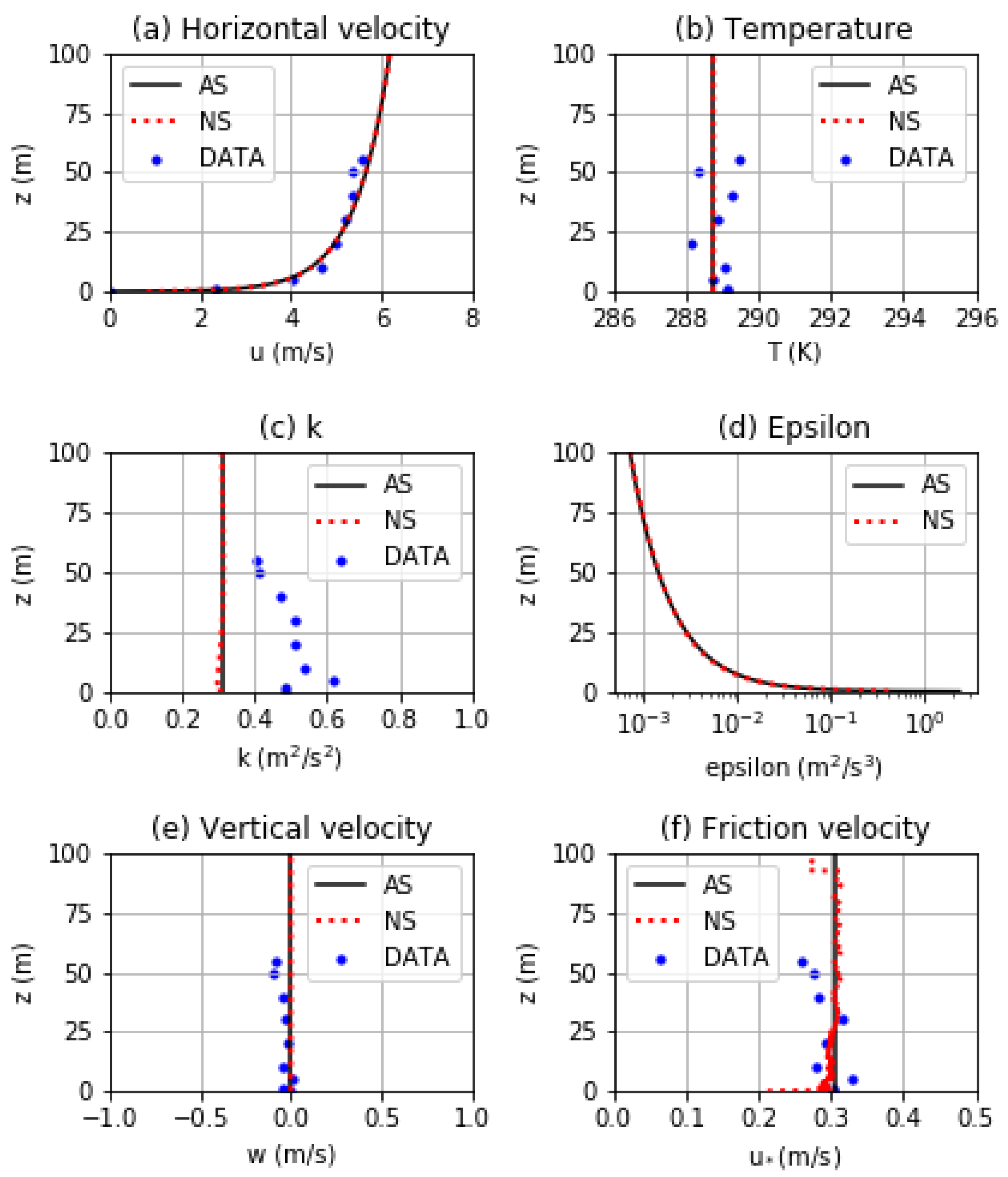
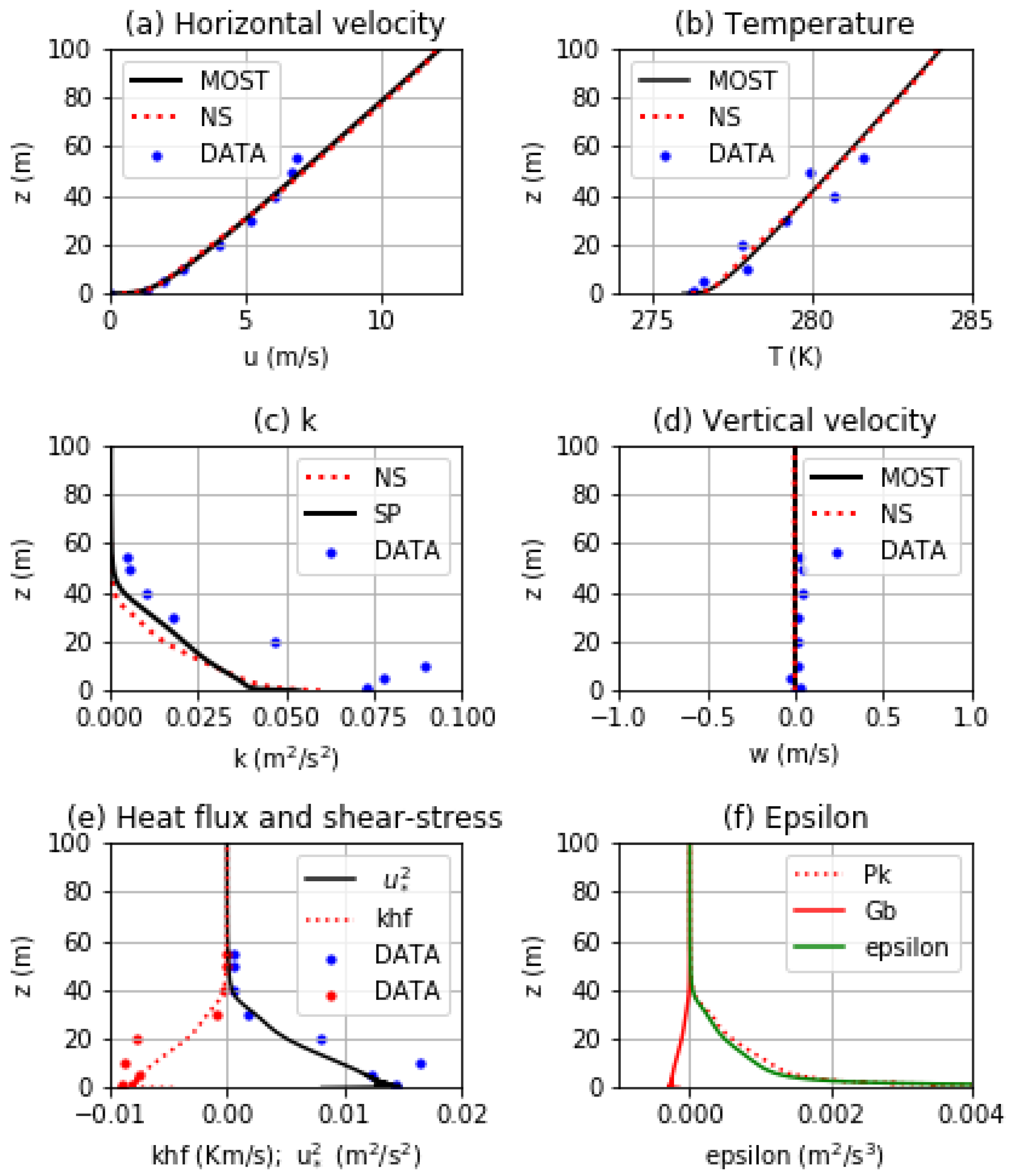
• The theoretical reference profiles for u, θ, and k, which were applied as upwind boundary conditions, were successfully reproduced by using CFD for the NBL. For the SBL, the reference MOST profiles were successfully reproduced for u and θ, as was the reference profile obtained by experiment in the case of k.
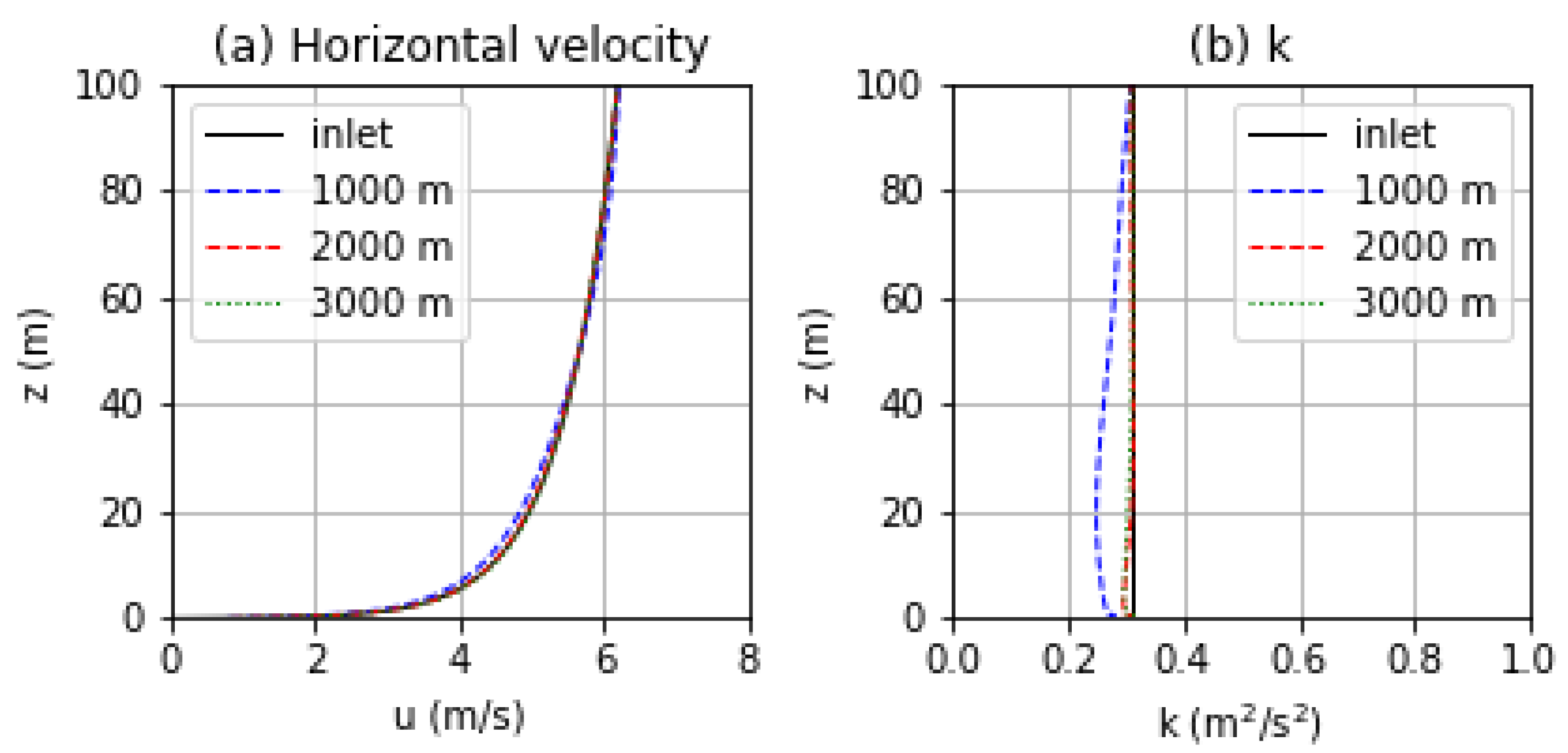
• Reference profiles were maintained throughout the computational domain for both u and θ. It took some distance for k to fully reach the equilibrium situation, especially for the NBL; but, thereafter, k was sustained in the domain and matched the respective upwind reference profiles. Small errors in the velocities were thought to affect k.
• The CASES-99 observations of u and θ can be adequately reproduced with CFD for the test cases; k showed less agreement with the observations, and possible reasons for this were considered.
• Reasonable agreement of the numerical results with the observed surface layer depth, and the profiles of shear stress and heat flux were obtained for the SBL.

References

1. Stull, R. An Introduction to Boundary Layer Meteorology; Springer: New York, NY, USA, 2009. [Google Scholar]
2. Richards, P.J.; Hoxey, R.P. Appropriate boundary conditions for computational wind engineering models using the k-ε turbulence model. J. Wind. Eng. Ind. Aerodyn. 1993, 46–47, 145–153. [Google Scholar] [CrossRef]
3. Richards, P.J.; Norris, S.E. Appropriate boundary conditions for computational wind engineering models revisited. J. Wind. Eng. Ind. Aerodyn. 2011, 99, 257–266. [Google Scholar] [CrossRef]
4. Yang, Y.; Gu, G.; Chen, S.; Jin, X. New inflow boundary conditions for modelling the neutral equilibrium atmospheric boundary layer in computational wind engineering. J. Wind. Eng. Ind. Aerodyn. 2009, 97, 88–95. [Google Scholar] [CrossRef]
5. Hargreaves, D.M.; Wright, N.G. On the use of the k-ε model in commercial CFD software to model the neutral atmospheric boundary layer. J. Wind. Eng. Ind. Aerodyn. 2007, 95, 355–369. [Google Scholar] [CrossRef]
6. Parente, A.; Gorle, C.; van Beeck, J.; Bennoci, C. Improved k-ε model and wall function formulation for the RANS simulation of ABL flows. J. Wind. Eng. Ind. Aerodyn. 2011, 99, 267–278. [Google Scholar] [CrossRef]
7. Alinot, C.; Masson, C. k-epsilon model for the atmospheric boundary layer under various thermal stratifications. J. Sol. Energy Eng. 2005, 127, 438–443. [Google Scholar] [CrossRef]
8. Chang, C.-Y.; Schmidt, J.; Dorenkamper, M.; Stoevesandt, B. A consistent steady state simulation method for stratified atmospheric boundary layer flows. J. Wind. Eng. Ind. Aerodyn. 2018, 172, 55–67. [Google Scholar] [CrossRef]
9. Optis, M.; Monahan, A.; Bosveld, F.C. Moving beyond Monin-Obuhkov similarity theory in modelling wind speed profiles in the lower atmospheric boundary layer under stable stratification. Bound.-Layer Meteorol. 2014, 153, 497–514. [Google Scholar] [CrossRef]
10. Launder, B.E.; Spalding, D.B. The numerical computation of turbulent flows. Comput. Method Appl. Mech. 1974, 3, 269–289. [Google Scholar] [CrossRef]
11. OpenFOAM. Available online: https://www.openfoam.com/ (accessed on 7 June 2021).
12. Nozaki, F. Available online: http://caefn.com/openfoam/solvers-buoyantpimplefoam/ (accessed on 7 June 2021).
13. Versteeg, H.; Malalasekera, W. An Introduction to Computational Fluid Dynamics: The Finite Volume Method; Pearson Education Limited: London, UK, 2007. [Google Scholar]
14. Li, D. Turbulent Prandtl number in the atmospheric boundary layer—where are we now? Atmos. Res. 2019, 216, 86–105. [Google Scholar] [CrossRef]
15. CHAM. Available online: http://www.cham.co.uk/phoenics/d_polis/d_enc/turmod/enc_t341.htm/ (accessed on 7 June 2021).
16. Zeli, V.; Brethouwer, G.; Wallin, S.; Johansson, A.V. Consistent boundary-condition treatment for computation of the atmospheric boundary layer using the explicit algebraic Reynolds-stress model. Bound.-Layer Meteorol. 2019, 171, 53–77. [Google Scholar] [CrossRef] [Green Version]
17. Poulos, G.S.; Blumen, W.; Fritts, D.C.; Lundquist, J.K.; Sun, J.; Burns, S.P.; Nappo, C.; Banta, R.; Newsom, R.; Cuxart, J.; et al. CASES-99: A Comprehensive Investigation of the Stable Nocturnal Boundary Layer. Bull. Am. Meteorol. Soc. 2002, 83, 555–581. [Google Scholar] [CrossRef]
18. 5 Minute Statistics of ISFF Data during CASES-99 Version 1.0. 2016, UCAR/NCAR—Earth Observing Laboratory. Available online: https://www.eol.ucar.edu/field_projects/cases-99/ (accessed on 7 June 2021).
19. Cheng, Y.; Oarlange, M.B.; Brutsaert, W. Pathology of Monin-Obukhov similarity in the stable boundary layer. J. Geophys. Res. 2005, 110, 1–10. [Google Scholar] [CrossRef] [Green Version]
20. Vickers, D.; Mahrt, L. The Cospectral Gap and Turbulent Flux Calculations. J. Atmos. Ocean Technol. 2003, 20, 660–672. [Google Scholar] [CrossRef]
21. Yague, C.; Viana, S.; Maqueda, G.; Redondo, J.M. Influence of stability on the flux-profile relationships for wind speed, φm, and temperature, φh, for the stable atmospheric boundary layer. Nonlinear Processes Geophys. 2006, 13, 185–203. [Google Scholar] [CrossRef] [Green Version]
22. Taylor, P.; Laroche, D.; Wang, Z.-Q.; McLaren, R. Obukhov Length Computation Using Simple Measurements from Weather Stations and AXYS Wind Sentinel Buoys; WWOSC: Montreal, QC, Canada, 2014. [Google Scholar]
23. Emeis, S. Wind Energy Meteorology: Atmospheric Physics for Wind Power Generation; Springer Science & Business Media: New York, NY, USA, 2018. [Google Scholar]
Figure 1. Comparison of the numerical solution (NS) with the analytic solution (AS) for the NBL: (a) horizontal velocity, (b) potential temperature, (c) turbulent kinetic energy, (d) turbulence dissipation rate, (e) vertical velocity, and (f) friction velocity. The numerical results are shown for a position 2000 m from the upwind boundary of the domain. The CASES-99 data are also shown, where applicable.
Atmosphere 13 00221 g001
Figure 2. Comparison of the numerical profiles along the length of the domain, and the reference profile applied as the inlet boundary condition for the NBL: (a) horizontal velocity and (b) turbulent kinetic energy.
Atmosphere 13 00221 g002
Figure 3. Comparison of the numerical solution (NS) with the reference profiles (obtained from MOST) and the CASES-99 data, where applicable for the SBL: (a) horizontal velocity; (b) potential temperature; (c) turbulent kinetic energy–SP refers to the simulated reference profile; (d) vertical velocity; (e) kinematic heat flux (khf = –u* θ*) and shear-stress (u*2); and (f) numerical production and dissipation of k. The numerical results are shown for a position 2000 m from the upwind boundary of the domain.
Atmosphere 13 00221 g003
Publisher’s Note: MDPI stays neutral with regard to jurisdictional claims in published maps and institutional affiliations.