Article

Research on the Growth Mechanism of PM2.5 in Central and Eastern China during Autumn and Winter from 2013–2020

1
National Meteorological Centre, Beijing 100081, China
2
Chinese Academy of Meteorological Sciences, Beijing 100081, China
3
Beijing Municipal Weather Modification Office, Beijing 100089, China
*
Author to whom correspondence should be addressed.
Atmosphere 2022, 13(1), 134; https://doi.org/10.3390/atmos13010134
Submission received: 24 November 2021 / Revised: 7 January 2022 / Accepted: 10 January 2022 / Published: 14 January 2022
(This article belongs to the Special Issue Air Pollution in China)

Abstract

:
Haze is a majorly disastrous type of weather in China, especially central and eastern of China. The development of haze is mainly caused by highly concentrated fine particles (PM2.5) on a regional scale. Here, we present the results from an autumn and winter study conducted from 2013 to 2020 in seven highly polluted areas (27 representative stations) in central and eastern China to analyze the growth mechanism of PM2.5. At the same time, taking Beijing Station as an example, the characteristics of aerosol composition and particle size in the growth phase are analyzed. Taking into account the regional and inter-annual differences of fine particles (PM2.5) distribution, the local average PM2.5 growth value of the year is used as the boundary value for dividing slow, rapid, and explosive growth (only focuses on the hourly growth rate greater than 0). The average value of PM2.5 in the autumn and winter of each regional representative station shows a decreasing trend as a whole, especially after 2017, whereby the decreasing trend was significant. The distribution value of +ΔPM2.5 (PM2.5 hourly growth rate) in the north of the Huai River is lower than that in the south of the Huai River, and both of the +ΔPM2.5 after 2017 showed a significant decreasing trend. The average PM2.5 threshold before the explosive growth is 70.8 µg m−3, and the threshold that is extremely prone to explosive growth is 156 µg m−3 to 277 µg m−3 in north of the Huai River. For the area south of the Huai River, the threshold for PM2.5 explosive growth is relatively low, as a more stringent threshold also puts forward stricter requirements on atmospheric environmental governance. For example, in Beijing, the peak diameters gradually shift to larger sizes when the growth rate increases. The number concentration increasing mainly distributed in Aitken mode (AIM) and Accumulation mode (ACM) during explosive growth. Among the various components of submicron particulate matter (PM1), organic aerosol (OA), especially primary OA (POA), have become one of the most critical components for the PM2.5 explosive growth in Beijing. During the growth period, the contribution of secondary particulate matter (SPM) to the accumulated pollutants is significantly higher than that of primary particulate matter (PPM). However, the proportion of SPM gradually decreases when the growth rate increases. The contribution of the PPM can reach 48% in explosive growth. Compared to slow and rapid growth, explosive growth mainly occurs in the stable atmosphere of higher humidity, lower pressure, lower temperature, small winds, and low mixed layers.

1. Introduction

Regional-scale, high-concentration aerosols are important causes of haze in central and eastern China [1,2]. Among a variety of pollutants, high concentrations of PM2.5 are still the most important aerosol pollutant, as well as the main cause of haze [3,4,5]. Elevated PM2.5 affects human health, the environment, and even climate [6,7]. The main causes that affect the production and consumption of PM2.5 include chemical reaction processes, meteorological factors, and emission sources [8,9,10]. When the emission source is stable, the temporal and spatial characteristics of air pollution mainly depend on meteorological factors [11]. The meteorology can influence the particulate matter (PM) evolution through many ways, e.g., secondary formation, accumulation or dilution, liquid-phase and heterogeneous reactions to secondary aerosols, etc. [12,13]. Under adverse atmospheric diffusion conditions, generally characterized by weak wind speeds, high relative humidity (RH), and low planetary boundary layer height, PM2.5 can quickly accumulate to a very high concentration [8]. The study by Zhang et al. [14] shows that the unfavorable weather elements in the winter of Beijing-Tianjin-Hebei can cause the PM2.5 concentration to increase by about 40% to 100% compared with other seasons. In light of single meteorological elements, Sun et al. revealed that, at low RH levels (<50%), PM increases linearly as a function of RH, among which OAs present the largest mass increase rate at 11.4 mg m−3/10% RH during wintertime in Beijing. In addition, the secondary formation is also one of the most important factors for the occurrence and development of haze weather [15]. Quan et al. [16] found that the conversion from NOx and SO2 to nitrate and sulfate was likely accelerated, and that both significantly increased in haze events. The secondary formation also promotes the formation of organic aerosols under certain conditions, and the rapid formation of secondary OA (SOA) under strong photochemical reactions can lead to more serious air pollution [17,18].
As a result of large reductions in anthropogenic emissions, the air pollution has been significantly improved with the successful implementation of “Action Plan on Prevention and Control of Air Pollution” in 2013 in China [19]. However, severe haze episodes still happen in some areas of central and eastern China (including Beijing-Tianjin-Hebei [10], Yangtze River Delta [20], Sichuan-Chongqing area [21], Fenwei Plain [22], Central China [23], etc.) in autumn and winter. For example, the rapidly spread coronavirus disease limited people’s outdoor activities and, hence, caused substantial reductions in anthropogenic emissions in 2020; however, there are still two persistent heavy pollution incidents from January 25 to 28 and February 8 to 14 in Beijing [24].
In heavy haze pollution, pollutants exhibit different growth rates at various stages of accumulation. Under different meteorological conditions, they may exhibit slow growth or rapid growth, and may increase by tens or even hundreds in one hour or several hours called “explosive growth” in the later stage of pollution. There is no qualitative conclusion about the cause of the rapid and even explosive growth of PM2.5. Zheng et al. [25] highlight that the trans-regional transportation of pollutants has led to a rapid increase in pollution. Wang et al. [26] believed that the secondary transformation and nucleation effect of aerosols played a more important role through simulation studies. The study by Zhong et al. [13] attributed the rapid increase in pollution more to the effect of meteorological factors, and their study concluded that more than 70% of the increase in PM2.5 can be attributed to the feedback effect after the persistent deterioration of the boundary layer meteorological conditions. Zhong et al. [27] conducted a study of 28 pollution episodes in Beijing from 2013 to 2017 and concluded that a threshold value for PM2.5 explosive growth is 100 μg m−3 in Beijing. Above this threshold, the positive feedback from aerosols to near-ground radiative cooling to anomalous inversion is effectively triggered. However, faced with the decreasing PM2.5 concentration year by year, this threshold may change over time and show some geographical differences. Regional emission controls were effective in reducing the PM2.5 mass concentration. However, the changes in SOA and inorganic aerosol were comparably small and even had slight increases [24]. Therefore, exploring the chemical component contribution and particle size evolution of aerosol particles is of great significance for further understanding the growth characteristics and physicochemical mechanism of PM2.5. In this study, ground-based PM2.5 observation data and meteorological element data are used to discuss the thresholds and year-on-year changes of PM2.5 in several major polluted areas in China from 2013 to 2020 under three growth mechanisms (slow, rapid, and explosive). The correlation between meteorological elements and the accumulation rate of pollutants is also discussed. At the same time, using the PM chemical composition and particle size distribution data, the contribution of PM composition and size distribution at different rates of pollutant cumulative stage is analyzed.

2. Materials and Methods

The following data are used in this study. (1) Hourly PM2.5 mass concentration from 2013 to 2020 in autumn and winter (October of the current year to February of the following year) is obtained by controlled stations of the Ministry of Environmental Protection in Northeast China (including Harbin (HEB), Changchun (CC) and Shenyang (SY)), Beijing-Tianjin-Hebei and surrounding areas (including Beijing (BJ), Tangshan (TS), Shijiazhuang (SJZ), Xingtai (XT), Jinan (JN) and Zhengzhou (ZZ)), Feiwei Plain (LinFen (LF), BaoJi (BaJ), XiAn (XA)), Yangtze River Delta (Nanjing (NJ), Hefei (HF), Shanghai (SH), Hangzhou (HZ)), Sichuan-Chongqing (Chengdu (CD) and Chongqing (CQ)), Central China (Wuhan (WH), Huangshi (HS), Nanchang (NC) and Changsha (CS)) and Pearl River Delta (Guangzhou (GZ), Shenzhen (SZ), and Zhuhai (ZH)). The data used were the mean values of urban observation stations. The geographical location of the relevant stations is shown in Figure 1. (2) To match the above area, the hourly conventional meteorological element data, including wind speed, relative humidity, wind direction, pressure, temperature etc., are provided by National Meteorological Information Center of the China Meteorological Administration (urban stations average). The time resolution of meteorological elements is 1 h. In order to more intuitively show the growth periods of PM2.5, taking Beijing as an example, Figure A1 in Appendix A shows the time series of PM2.5 and meteorological elements in January 2015 in Beijing. Furthermore, the average diurnal of PM2.5 and meteorological variables from 2013 to 2020 in autumn and winter in Beijing is shown in Figure A2. (3) The chemical composition data of submicron PM (PM1) were sampled from Institute of Atmospheric Physics (IAP, 39°58′28″ N, 116°22′16″ E), an urban site located between the north 3rd and 4th ring road in Beijing (Jiang et al., 2015). The sampling time was October 2012 to February 2013. The sampling instrument was the Aerosol Chemical Speciation Monitor (ACSM), with a time resolution of ~15 min. ACSM mainly detects particles below 1 μm, which can realize real-time online determination of OA, sulfate (SO42−), nitrate (NO3), ammonium salt (NH4+), and chloride (Chl). The detailed description of the relevant instrument principles and parameters of the ACSMs have been to the references of Sun et al. [28] and Ng et al. [29]. At vaporizer temperature of ~600 °C, the ACSM cannot detect refractory materials, e.g., mineral dust and black carbon (BC). Thus, an aethalometer (Model AE22, Magee Scientific Corporation, Berkeley CA, USA) is used to simultaneously measure BC in PM2.5. The PM2.5 and gaseous species (including CO, SO2, NO, NOx, and Ox) were measured by a heated Tapered Element Oscillating Microbalance (1400a, Thermo Scientific, Waltham, MA, USA) and various gas analyzers (Thermo Scientific). (4) The data of aerosol number spectrum from 27 November 2014 to 28 February 2015, with a time resolution of 3 min and a measurement range of 14.6 nm to 661.2 nm, were measured by an scanning mobility particle sizer (SMPS), provided by the Beijing Meteorological Bureau, China. (5) The PM2.5 grid distribution data come from a 1-km-resolution PM2.5 dataset, called China High Air Pollutants (CHAP, https://weijing-rs.github.io/product.html (accessed on 18 September 2021)) from 2013 to 2020 across China, generated by the Moderate Resolution Imaging Spectroradiometer (MODIS, MODIS Collection 6 MAIAC AOD product (MCD19A2)) and multi-angle implementation of the atmospheric correction (MAIAC) algorithm (Wei et al., 2021). The inversion method is the space–time extra-trees (STET) model with high accuracies (i.e., cross-validation coefficient of determination, CV-R2 = 0.86–0.90) and strong predictive powers (i.e., R2 = 0.80–0.82) [30].
The Roche method is used to calculate the height of the atmospheric mixing layer height (MLH). It is a method proposed by Nozaki et al. [31] in 1973 to estimate the height of the mixed layer using ground meteorological data. This method takes into account that the atmospheric mixing layer is the result of the combined action of thermal and dynamic turbulence. Moreover, the movement of the atmosphere in the upper boundary layer often interconnect and feedback with ground meteorological elements, so ground meteorological parameters can be used to estimate the height of the mixed layer. In addition, positive matrix factorization (PMF) [32] was preformed to resolve distinct OA factors from specific sources on ACSM mass spectra. The related principles and steps of this method are detailed in Ulbrich et al. [33] and Decarlo et al. [34]. In this study, we limit PMF analysis to m/z 12–125 considering the low contribution of m/z 125–150 to the total signal. An Igor Pro-based PMF evaluation tool (PET, v 2.04) is used to further evaluated the results of PMF.

3. Results and Discussion

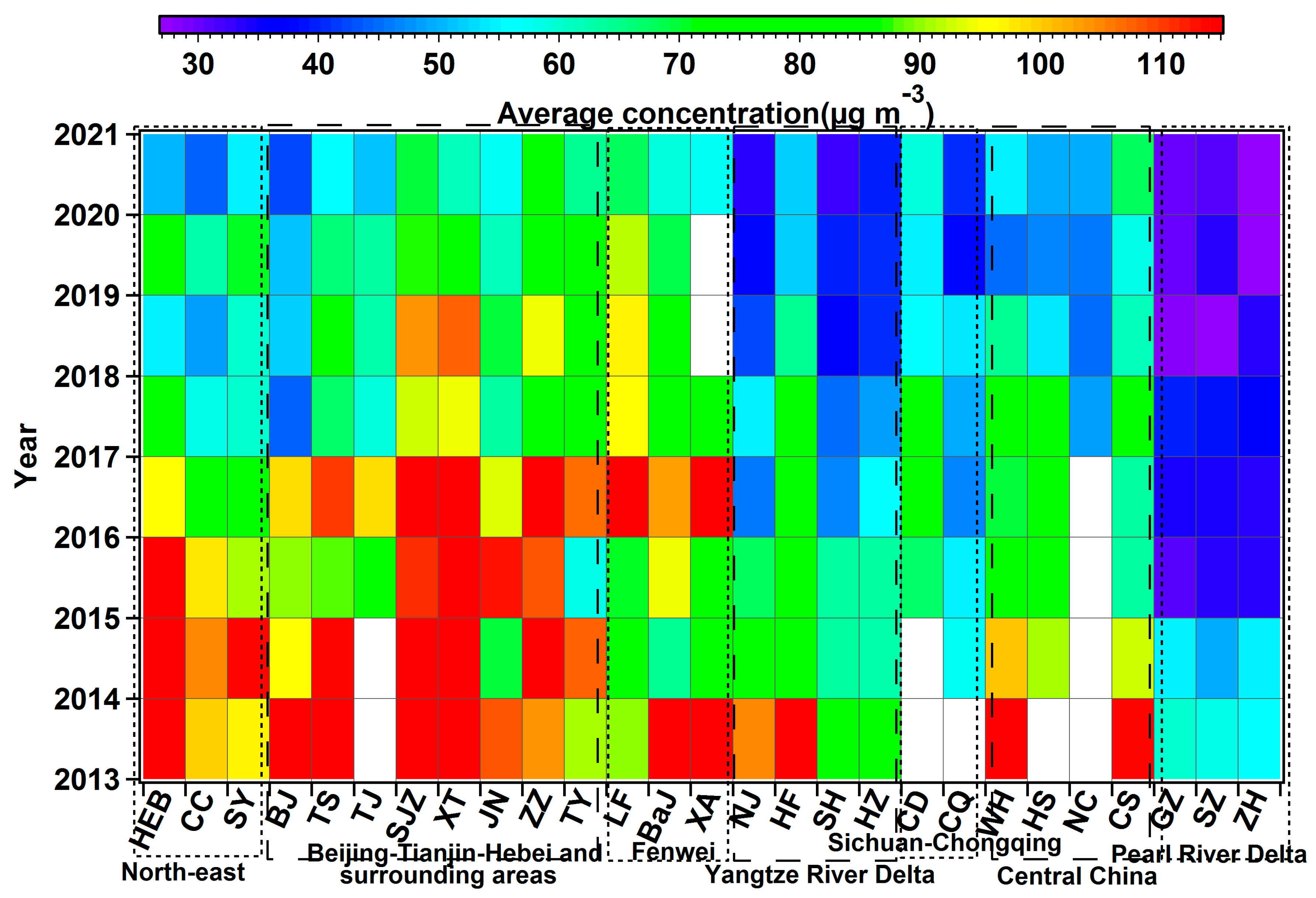
3.1. Average Distribution of PM2.5 in Autumn and Winter of China from 2013 to 2020

Figure 1 shows the average distribution of PM2.5 mass concentration in the autumn and winter (October of the current year to February of the following year) of 2013–2020 based on satellite inversion in the central and eastern of China. On average, Northeast China, Beijing-Tianjin-Hebei, and surrounding areas (Fenwei, Yangtze River Delta, Sichuan-Chongqing, Central China, and Pearl River Delta (seven regions)) are the major areas where PM2.5 concentration is relatively high in China. The following research on the growth law of PM2.5 is also mainly carried out for the above-mentioned regions and representative cities.
We carried out annual statistics on the average concentration of PM2.5 in autumn and winter (Hereinafter refers to as average PM2.5 concentration) of selected representative stations since 2013. As shown in Figure 2, from the perspective of the evolution of the time series, since 2013, the PM2.5 of the seven regional representative stations shows an overall decreasing trend. For the three regional representative stations of Northeast China, Beijing-Tianjin-Hebei and surrounding areas and Fenwei (north of the Huai River in China), the pollution of PM2.5 in autumn and winter is significantly lower after 2016 than before. From 2013 to 2016, 30% of the representative stations in the above three regions had an average PM2.5 mass concentration more than 115 µg m−3 (115 µg m−3 is the limit concentration of average daily moderate pollution stipulated by the Ministry of Environmental Protection of the People’s Republic of China), and 87% of statistical values exceed 75 µg m−3 (the second grade of NAAQS released in 2012 by the Ministry of Environmental Protection of the People’s Republic of China, http://kjs.mep.gov.cn/hjbhbz/bzwb/dqhjbh/dqhjzlbz/201203/t20120302224165.htm (accessed on 7 September 2021)). The highest average value of PM2.5 exceeds 200 µg m−3 (Shijiazhuang in 2013). However, in the autumn and winter from 2017 to 2020, the average PM2.5 concentration is lower than 115 µg m−3, and only 30% of sites have an average PM2.5 more than 75 µg m−3 north of the Huai River. Especially by 2020, the statistics of all sites in the three regions are lower than 75 µg m−3.
The other four areas with a lower latitude south of the Huai River in China (Yangtze River Delta, Sichuan-Chongqing, Central China, and Pearl River Delta) have significantly less fine particulate pollution than the three areas north of the Huai River (Northeast, Beijing-Tianjin-Hebei and surrounding areas, and Fenwei). Among the valid data, except for HF and WH in 2013, which average PM2.5 concentration exceeded 115 µg m−3, other statistical values are all lower than 115 µg m−3. For the Pearl River Delta region, after 2015, the average PM2.5 value was lower than 35 µg m−3 (24-h NAAQS of US EPA). Among sites south of the Huai River, the proportion of average PM2.5 concentration exceeds 75 µg m−3, which accounts for 26% from 2013 to 2017. However, from 2018 to 2020, the average of PM2.5 is all below 75 µg m−3. A number of studies showed that the main reason for the gradual decrease in the concentration of PM2.5 in central and eastern China is the decrease in the concentration of gaseous precursors under the joint emission controls and, hence, the suppression of secondary growth and formation [35,36]. However, many studies have also pointed out the importance of meteorological conditions, which can help to explain the reduction in PM2.5 concentration of over 50% [14]. The combined effect of meteorological factors and anthropogenic emissions makes the cause of air quality improvement still uncertain [37]. The main reason that the PM2.5 concentration in the north of Huaihe River is higher than that in the south of the Huaihe River is the comprehensive effect of industrial layout, industrial structure, meteorological factors (precipitation, atmospheric diffusion conditions), and topography, etc.

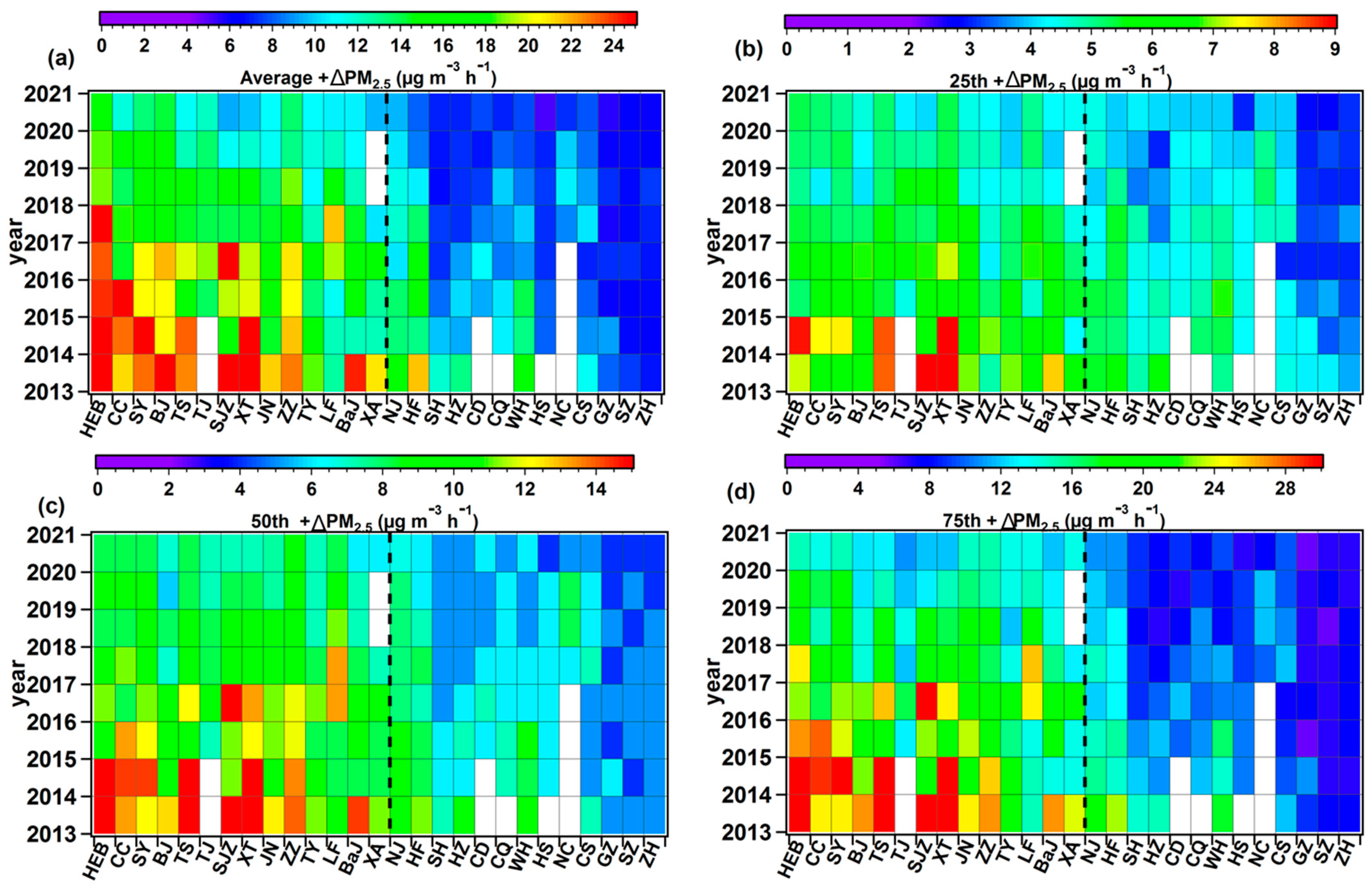
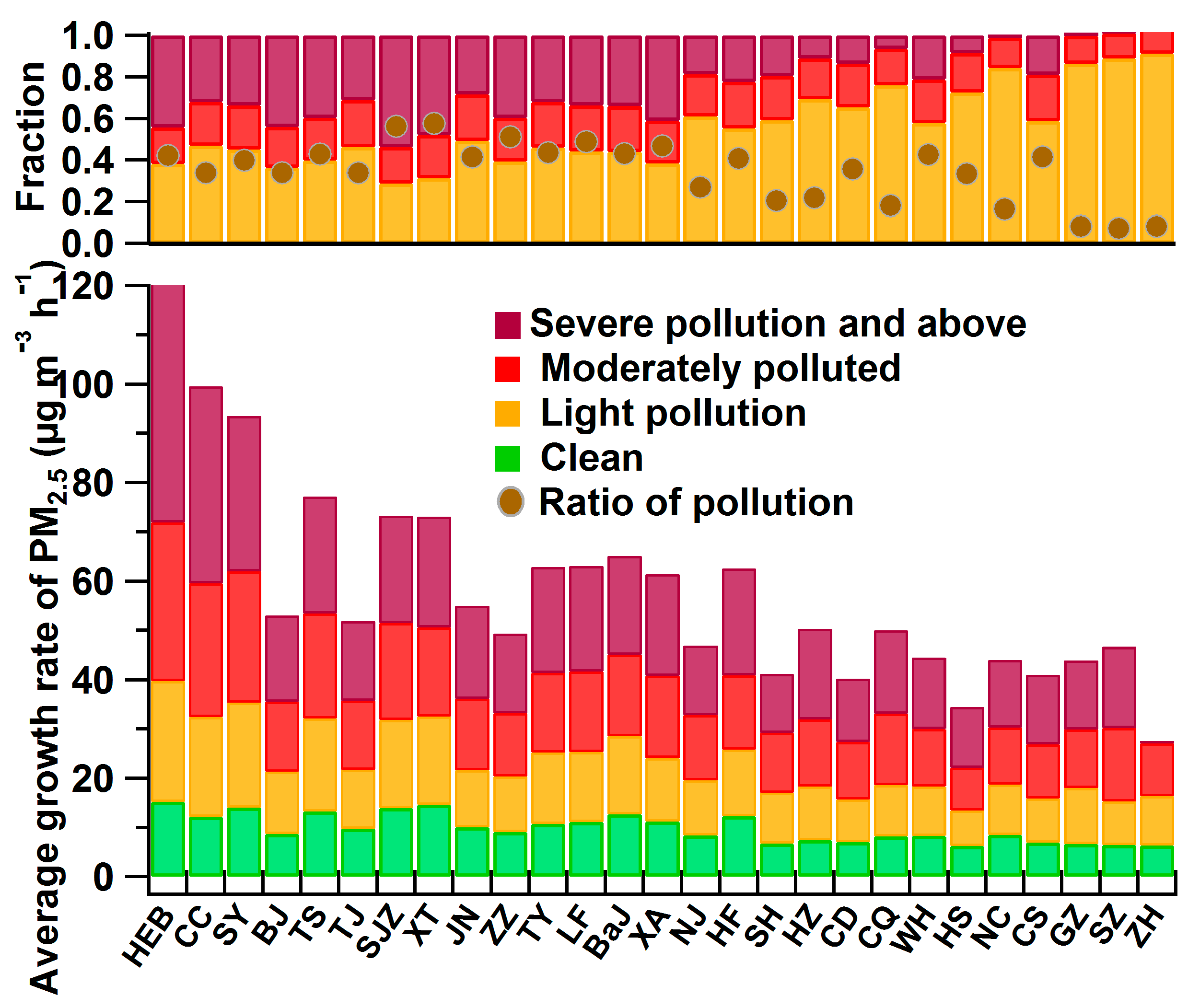
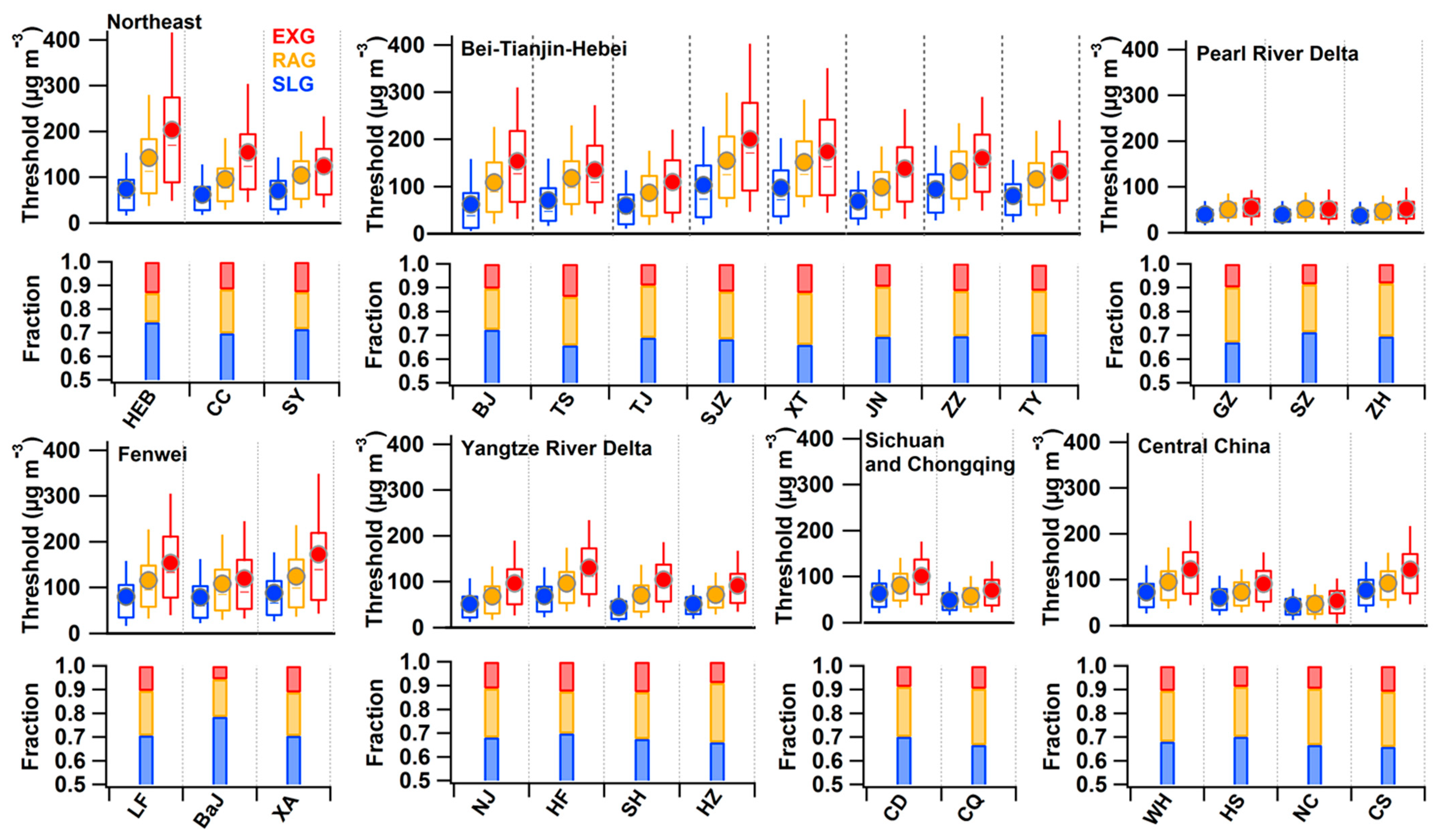
3.2. Classification of PM2.5 Growth Periods in Central and Eastern China form 2013 to 2020

To explore the growth mechanism of PM2.5 in autumn and winter, the data of PM2.5 growth periods (GP, hourly growth rate > 0) from 2013 to 2020 were selected year by year. Unless otherwise specified, the following research only focuses on the hourly growth rate greater than 0, that is, the data during the positive GP. The hourly growth rate of PM2.5 (unit: µg m−3/h) is expressed as +ΔPM2.5. Figure 3 shows the statistical value of +ΔPM2.5 at different representative stations in autumn and winter year by year. Similar to the average PM2.5 concentration, with the Huai River as the boundary, the +ΔPM2.5 of the representative station in the southerly latitude area is lower than that of the northerly latitude station (autumn and winter). In terms of average value, the mean range of +ΔPM2.5 north of the Huai River is 10.7–40.9 µg m−3/h between 2013 to 2017 (on the left side of the dotted line). Among them, the maximum value of 40.9 µg m−3/h appeared in the Harbin (Northeast China) in 2013. Except for Shijiazhuang and Changchun, the average +ΔPM2.5 of 12 of the 14 sites (north of Huai river) in 2015–2016 was lower than that in 2013 and 2014. However, the +ΔPM2.5 of eight sites rebounded in 2016 comparing to 2015. After 2017, +ΔPM2.5 has a stepwise decline. Except for Linfen (Fenwei) and Harbin (Northeast China), whose +ΔPM2.5 is 27.2 and 21.5 µg m−3/h, respectively, all other stations decreased by less than 19 µg m−3/h. Especially in 2021, the maximum value of +ΔPM2.5 is only 15.3 µg m−3/h with a relatively concentrated distribution range of each site between 15.3 µg m−3/h and 9.4 µg m−3/h. For the representative stations south of the Huai River (on the right side of the dotted line), the average of +ΔPM2.5 is less than 20 µg m−3/h except for Hefei in 2013, which was 21.6 µg m−3/h. After 2017, all stations of +ΔPM2.5 educe to within 15 µg m−3/h and within 10 µg m−3/h in 2020.
The statistical results of the 25th, 50th, and 75th percentiles of +ΔPM2.5 are similar to the average overall. The distribution value of +ΔPM2.5 in the north of the Huai River is lower than that in the south of the Huai River, and the +ΔPM2.5 after 2017 also showed a significant decreasing trend compared with that before 2017. In the statistical results, the value of the 50th (median value) of the +ΔPM2.5 is significantly lower than that of the average, indicating that values greater than the 50th deviate are higher than those less than the 50th.
The PM2.5 concentration before the start of growth is classified with 75 µg m−3 as the boundary, divided into clean and pollution, of which pollution is further divided into light (75–115 µg m−3), moderate (115–150 µg m−3), and heavy pollution (>150 µg m−3). The +ΔPM2.5 is compared based on the PM2.5 background mass concentration (clean, lightly polluted, moderately polluted, and severely polluted) before the start of the growth. At the same time, the proportions of pollution background, as well as the proportions of light, moderate, and severe pollution (under pollution background) before the start of growth, are shown in Figure 4. Still using the Huai River as the division, the proportion of PM2.5 growth occurring in the pollution background in south of the Huai River is significantly lower than that of the sites north of the Huai River. Among the representative stations in the Pearl River Delta, only 7–8% of PM2.5 growth occurred in pollution. Among other representative stations south of the Huai River, the highest probability of PM2.5 growth occurring in the pollution is Wuhan (42.0%), followed by Nanjing (40.0%) and Changsha (40.1%). Other sites are all below 40%. For the 14 representative stations north of the Huai River, the proportion of the PM2.5 increase in pollution is higher than 33%, and 78.6% of the stations are higher than 40%. For the stations of Shijiazhuang and Xingtai, in particular, the proportion of pollution background is as high as 55.5% and 56.8%, respectively. Further classifying pollution into light, moderate, severely pollution, as indicated in Figure 4, in the pollution background, the sites south of the Huai River are dominated by light pollution, with the lowest being 55% (Hefei) and an average of 71.2%. In contrast, more than 50% of the PM2.5 growth occurs in moderate and heavy pollution in the pollution background of the stations north of the Huai River. It is noteworthy that the proportion of heavy pollution is significantly higher than that of moderate, especially for Shijiazhuang and Xingtai, where the proportion of the PM2.5 growth occurs in heavy pollution (53.7% and 48.0%, respectively) once the light pollution is exceeded.
The average of +ΔPM2.5 corresponding to clean, light pollution, moderate pollution, and heavy pollution background was calculated before growth in GP (Figure 4 below). It can be seen from Figure 4 that, among all representative stations, the average of +ΔPM2.5 corresponding to the clean background before GP is the lowest, followed by light, moderate, and heavy pollution. Among them, the average of +ΔPM2.5 under a clean background generally less than 15 µg m−3 and the increase value is generally under 10 µg m−3 h−1 in most areas south of the Huai River. Under the background of light pollution, the distribution range of the average +ΔPM2.5 at stations north of the Huai River is between 11.2 µg m−3 h−1 and 24 µg m−3 h−1, with an average of 16.1 µg m−3 h−1. South of the Huai River is slightly lower, with an average of 10.2 µg m−3 h−1 of +ΔPM2.5 under a light pollution background. Under moderate and severe backgrounds, the average +ΔPM2.5 at stations north of the Huai River were 19.0 µg m−3 h−1 and 26.6 µg m−3 h−1, respectively. The average +ΔPM2.5 south of the Huai River (moderate: 12.3 µg m−3 h−1, severe: 15.1 µg m−3 h−1) is significantly lower than that in the north of the Huai River, but still higher than the average +ΔPM2.5 under the background of clean and light pollution of the site. Therefore, in each regional representative site, the background concentration of PM2.5 before GP has an important impact on the PM2.5 growth rate. Overall, a higher degree of air pollution before the growth leads to a faster average growth rate of the PM2.5.
The PM2.5 shows different growth rates during GP (+ΔPM2.5 > 0). According to the value of +ΔPM2.5, we divided GP into three categories as slow growth (SLG), rapid growth (RAG), and explosive growth (EXG). The atmosphere aerosol background concentration and the growth rate of PM2.5 both show obvious regional and inter-annual differences (Figure 2, Figure 3 and Figure 4). We define the average annual +ΔPM2.5 from 2013 to 2020 as the threshold Ak,year (K represents the region) for determining the type of growth (SLG, RAG, or EXG) of the stations in that year. Figure 3a shows the value of Ak,year. Slow growth (SLGk, year), defined as the +ΔPM2.5, is less than Ak, i.e., SLGk, year < Ak,year; the interval of rapid growth (RAGk, year) is between 1 and 2 times of Ak,year, i.e., Ak,year ≤ RAGk, year ≤ 2* Ak,year; and the +ΔPM2.5 of explosive growth (EXGk, year) is more than double that of the threshold, i.e., EXGk, year > 2* Ak,year.
Since the +ΔPM2.5 in GP is closely related to the initial PM2.5 concentration, there should be a certain PM2.5 concentration threshold to judge the rapid or even explosive growth of PM2.5. Zhong et al. [13] found that, when PM2.5 reached a certain threshold, the positive feedback from aerosols to near-ground radiative cooling to anomalous inversion is effectively triggered, which subsequently results in explosive rising of PM2.5. In each representative station, the proportion of EXG in GP is 6.2–13.8%, with an average of 10.3% (Figure 5). Among them, the EXG of Tangshan (Beijing-Tianjin-Hebei and surrounding areas) accounted for more than 20% of the GP, which was the highest among all representative stations. Although the proportion of the EXG is lower than the RAG and the SLG, the EXG played a vital role in the occurrence and development of the heavy pollution process. It is necessary to quantify the relevant threshold of the EXG.
Figure 5 presents the average PM2.5 concentration thresholds before EXG in representative stations in each region during autumn and winter from 2013 to 2020. The statistical value of the lower quartile (25th) of PM2.5 before EXG can be used as the reference threshold of PM2.5 concentration for EXG, and the upper quartile (75th) characterizes that exceeding this critical value is extremely prone to EXG [13,27]. In the relatively heavily polluted stations north of the Huai River, the average PM2.5 threshold before the EXG is 70.8 µg m−3. Among them, the threshold in Beijing is 68.3 µg m−3, which is slightly lower than the strict threshold (71 µg m−3) proposed by Zhong et al. [13] for the EXG of PM2.5 in Beijing. The stations with the highest EXG threshold is Shijiazhuang (91.0 µg m−3), followed by Harbin (89.1 µg m−3) and Zhengzhou (88.9 µg m−3). Although the PM2.5 concentration threshold is the highest, the probability of EXG in these three cities (Shijiazhuang, Harbin and Zhengzhou) is still higher than the average proportion in the north of the Huai River (11.5%). For the area south of the Huai River, air pollution is relatively light, but at the same time, the threshold for PM2.5 explosive growth is relatively low, and a more stringent threshold also puts forward stricter requirements for atmospheric environmental governance. The upper quartile of the initial PM2.5 mass concentration values is much higher than the lower quartile (threshold) with the distribution interval from 156 µg m−3 to 277 µg m−3 for the area north of the Huai River. Beijing’s upper quartile value is 156 µg m−3, which indicates that an explosive growth of PM2.5 will likely occur once it is higher than this value.
As a comparison, the statistical values of SLG and RAG are lower than that of EXG, while the relevant thresholds can also be used as a stage indicator of prevention and control measures.

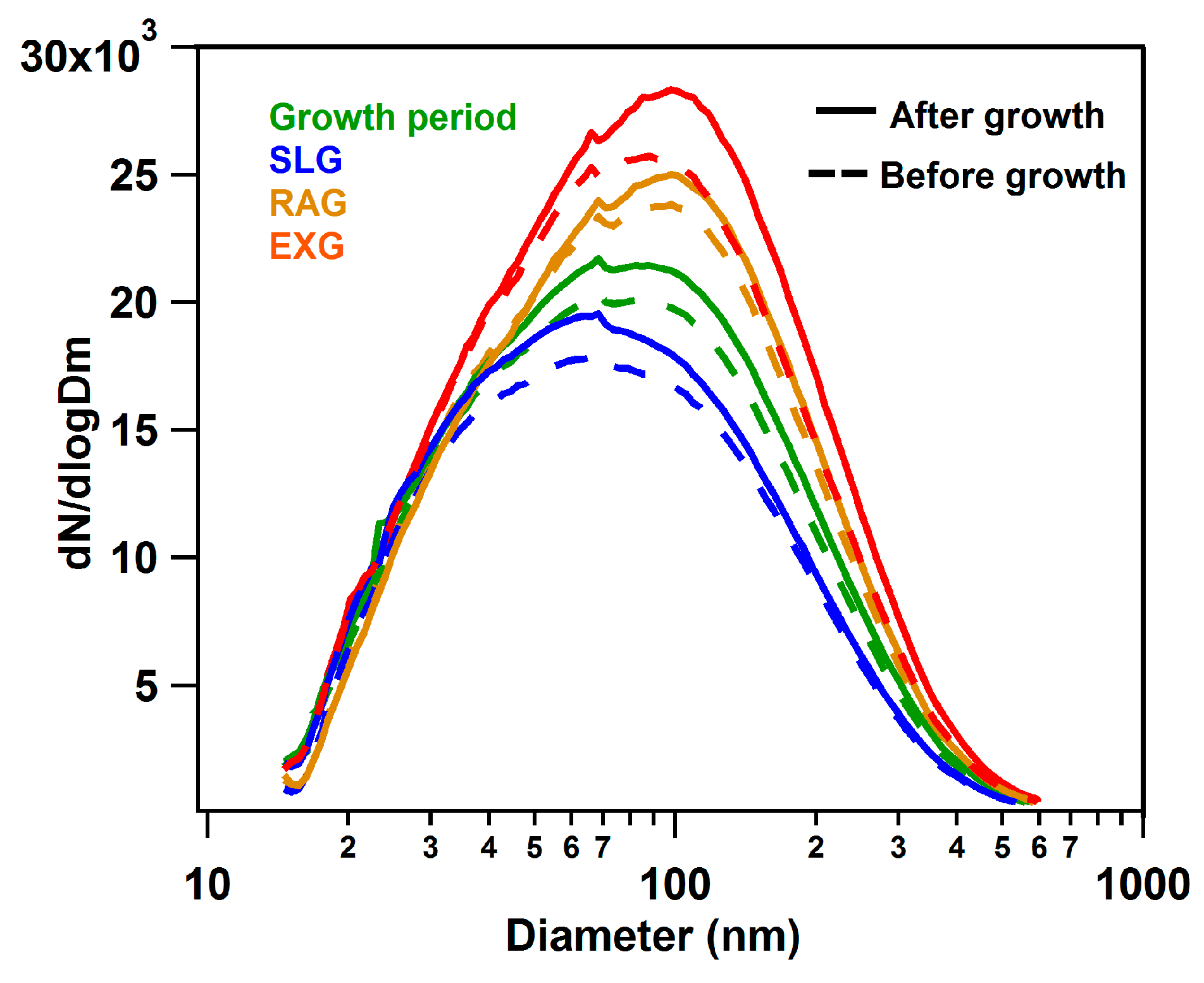
3.3. Size Distribution

Figure 6 shows a comparison of average size distributions before and after GP, SLG, RAG, and EXG in Beijing (27 November 2014 to 28 February 2015). As indicated in Figure 6, from SLG, RAG, to EXG, the peak number concentration gradually increasing. The peak number concentration spectrum distribution of GP is between SLG and RAG. After the growth started, the peak number concentration of the three growth rates all increased significantly. However, there is no significant difference in the peak number concentration particle size before and after the growth of the three growth ways. According to the definition of Hussein et al. (2004), different particle sizes could be divided into four modes: the nucleation mode (0.01~0.02 μm), the Aitken mode (0.02~0.1 μm), the accumulation mode (0.1~1 μm), and the coarse mode (1~10 μm) [38]. Limited by the measuring range of the instrument, the coarse mode is not studied in this article. In terms of the number of concentrations, before and after the three growth ways, the number concentration of the nucleation mode (NUM), the Aitken mode (AIM), and the accumulation mode (ACM) all show varying degrees of growth (Table 1). Among RAG and EXG, the increasing number concentration of AIM and ACM is more significant. Calculated from Table 1, during the SLG, the particles’ concentration growth rate of the NUM, AIM, and ACM are 1691/cm−3 h−1, 586/cm−3 h−1, and 325/cm−3 h−1, respectively. However, the growth rate of the number concentration of NUM decreases to 941/cm−3 h−1 and 668/cm−3 h−1 in the RAG and EXG, respectively. Simultaneously, the growth rate of AIM in the RAG and EXG is 3.5 times and 7.7 times higher than that of SLG, respectively. For the ACM, in particular, the growth rate in the EXG can reach 4483/cm−3 h−1 in Beijing during autumn and winter.
Comparing with the three growth rates, the peak diameters gradually shift to larger sizes with the growth rate increasing. The particle diameters corresponding to the peak concentration of SLG is ~65 nm, and the peak particle diameters of RAG and EXG grow to ~94 nm and ~103 nm, respectively. Since the growth rate of PM2.5 is closely related to the degree of air pollution, the average growth rate under pollution background is, on average, higher than that of clean conditions, which is similar to the results of Guo et al. [39], who showed that the average particle diameters of aerosols in Beijing gradually increase from cleaning to pollution with an average daily mass growth of 50~110 µg m−3. The study by Xu et al. [40] showed that the increased particle size of OA mainly corresponds to SOA, while the particle size of POA hardly changes. At the same time, the hygroscopicity parameter of OA increased substantially with particle size and has played a further role in promoting the increase in pollution.
Figure 7 shows the number concentration spectrum distribution of 12 times PM2.5 episodes in 2014 and 2015 during autumn and winter. In the cumulative phase of the pollution process, slow, rapid, and explosive growth alternately occur. Before reaching the peak concentration in most heavy pollution episodes (especially the peak concentration of PM2.5 exceeding 200 µg m−3), it is accompanied by an obvious explosive increase in PM2.5. Consistent with the above conclusions, when the EXG occurs, the number concentration of NUM does not increase significantly, and the particle size with increased concentration is mainly distributed in AIM and ACM. Since the growth rate of pollution is related to the mass concentration of PM2.5 (Section 3.2), the rapid and explosive growth usually occurs in severe air pollution. On the one hand, there is a noticeable absence of new particle formation as the pollution episode develops. On the other hand, with the stable atmospheric situation, small particles keep growing by collision and hygroscopic growth. While the NUM particles contribute negligibly to the particle mass concentration, the severe pollution episodes (high growth rate) are attributable to the presence of numerous large particles.

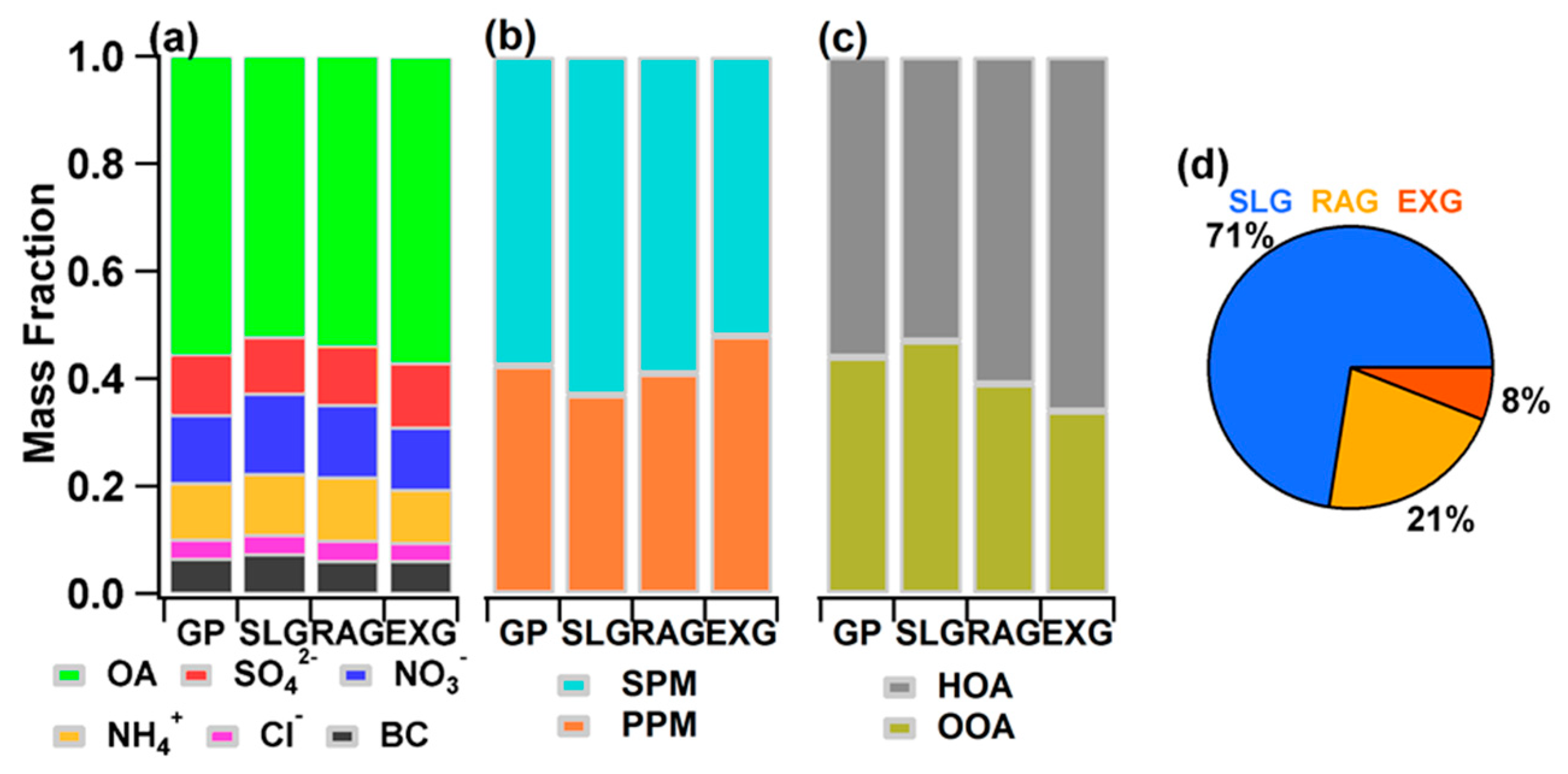
3.4. Chemical Composition

To explore the contribution of aerosol components in SLG, RAG, and EXG during autumn and winter in Beijing (October 2012 to February 2013), Figure 8a shows the average contribution of PM1 species (PM1 = OA + SO42− + NO3 + NH4+ + Chl + BC) to the increasing mass concentration in GP. Among the growing concentration of PM1, the contribution of OA exceeds 50% on average (discuss only in the increased concentration, same below). With the increase in +ΔPM2.5, in particular, the proportion of OA gradually increases. The contribution of OA to the EXG reaches 57.3%, which is significantly higher than the RAG (52.1%) and SLG (54.3%). Among the inorganic components (SO42− + NO3 + NH4+ + Chl), in addition to the EXG, NO3 contributes the most in SLG and RAG, followed by NH4+ and SO42−. However, when the growth rate increases, the contribution of NO3 gradually decreases, while the contribution of SO42− is the opposite. In the EXG, the contribution of SO42− is slightly higher than that of NO3, becoming the largest contributor to the inorganic components. Sun et al. [41] concluded that with the increase in relative humidity in autumn and winter, SO42 increased rapidly through liquid phase chemical reactions, while NO3 mainly existed in the form of particulate matter, gas-particle transformation was inhibited. Photochemical reactions during the day become the main production mechanism of NO3. It can be seen from Figure 9 that the relative humidity (RH) before the EXG is significantly higher than that of RAG and SLG. Higher RH accelerated the growth rate of SO42, resulting in a significant increase in the proportion of SO42 in the accumulated pollutants.
PMF analysis of ACSM mass spectra of OA identified two components, i.e., hydrocarbon-like OA (HOA) and oxygenated OA (OOA), as compared to the simultaneous observation of gas components (O3, SO2, NOx, and CO, etc.), and various organic source spectra. In this study, HOA is closely related to BC (a tracer for combustion emissions, r2 = ~0.63) and NOx (r2 = ~0.57), indicating the important contribution of vehicle sources. OOA has a high correlation with SO42− (r2 = ~0.68) and NO3 (r2 = ~0.77), which are both secondary inorganic species, indicating that OOA is driven by regional production mostly. In the RAG and EXG, POA (in this study = HOA) contributes more than 60% to the growth concentration of OA on average, which is significantly higher than the average proportion of POA in all growth periods (~55.8%) (Figure 8c). The high proportion of HOA is also reflected the important contribution of traffic sources to the accumulation of pollutants in the RAG and EXG. Contrary to the change in humidity, the average temperature before the EXG is the lowest among the three growth rates, followed by RAG (Figure 10b). Studies have shown that the decrease in temperature is conducive to the increase in POA mass concentration [42], which also partly explains the higher proportion of POA in the accumulated OA during the EXG. Therefore, among the various components of PM1, OA, especially POA, have become one of the most critical components for the EXG in Beijing during autumn and winter. In the GP, SOA (in this study = OOA) contributed 47.1% of OA in SLG. Furthermore, in the RAG and EXG, the contribution of SOA decreased to 39% and 34% on average. Figure 10 shows the mass spectra of average OA before and after GP and three growth ways. As illustrated, the intensities of hydrocarbon ion series of m/z 55 (mainly C3H3O+, C4H7+), m/z 57 (mainly C3H5O+, C4H9+), and m/z 43, characterized by a mass spectral pattern of HOA, show a significant increase after three growth ways. Among them, the growth intensity of EXG is higher than that of SLG and RAG. OOA is characterized by the prominent peak of m/z 44 (CO2+). Before and after growth, the intensities of m/z 44 decreased significantly. In the EXG, the intensity of m/z 44 decreases from 11.3% to 10.2% of the total OA signals. Although the proportion of SOA is significantly lower than that of POA in GP, the proportion of SOA in GP is significantly higher than the average observed throughout the autumn and winter (31%). The research of Xu et al. [40] also showed that SOA plays an enhanced role during more severely polluted days. Therefore, in the process of pollution accumulation, SOA also plays a vital role in the increase in OA.
Secondary aerosol (SPM = SO42− + NO3 + NH4+ + OOA) is the most important component of PM1, accounting for ~71% of PM1 in autumn and winter in Beijing on average, and has a significant impact on atmospheric extinction [43]. During the GP, the contribution of SPM to the accumulated pollutants is still significantly higher than that of PPM (Chl + BC + HOA). However, from slow to rapid to explosive growth, the proportion of SPM in the increased PM gradually decreases (63% to 59% to 52%) (Figure 8b). During the EXG, the contribution of the PPM can reach to 48% in the increasing concentration of pollutants. PPM mainly comes from local biomass combustion, traffic and catering emissions, and its contribution to pollution accumulation cannot be underestimated. Figure 8d shows that, during the observation period, the proportions of SLG, RAG, and EXG are 71%, 21%, and 8%, respectively, in Beijing during observation. Compared to SLG and RAG, EXG mainly occurs in the quiet and stable atmosphere of higher humidity, lower pressure, lower temperature, small winds, and low MLH (Figure 10).

4. Conclusions

We select a total of 27 representative stations in seven areas (Northeast China, Beijing-Tianjin-Hebei and surrounding areas, Feiwei Plain, Yangtze River Delta, Sichuan-Chongqing, Central China and Pearl River Delta) in central and eastern China to analyze the year-on-year evolution trend of PM2.5 pollution in the autumn and winter from 2013 to 2020. The increased stage of pollutants is divided into SLG, RAG, and EXG, according to the different accumulation rate of pollution. Taking Beijing as an example, a comparative study is conducted on the distribution characteristics of aerosol particle size, the contribution of chemical components, and the differences in meteorological conditions in three growth rates. The average value of PM2.5 in the autumn and winter of each regional representative station shows a decreasing trend as a whole, especially after 2017, where the decreasing trend was significant. The +ΔPM2.5 in the north of the Huai River is lower than that in the south of the Huai River, and the +ΔPM2.5 after 2017 also showed a significant decreasing trend compared with that before 2017. The average PM2.5 threshold before the EXG is 70.8 µg m−3, and the threshold that is extremely prone to EXG ranges from 156 µg m−3 to 277 µg m−3 in the stations north of the Huai River. For the area south of the Huai River, the threshold for PM2.5 EXG is relatively low, while a more stringent threshold also puts forward stricter requirements for atmospheric environmental governance. With the growth rate increase, the peak number concentration diameters gradually shift to a larger size in Beijing. The number concentration increasing mainly distributed in AIM and ACM during EXG. Among the various components of PM1, OAs, especially POA, have become one of the most critical components for the EXG of pollutants in Beijing. During the GP, the contribution of SPM to the accumulated pollutants is significantly higher than that of PPM. However, with the increase in growth rate, the proportion of SPM gradually decrease. In the EXG, the contribution of the PPM can reach up to 48%. Compared to SLG and RAG, EXG mainly occurs in the stable atmosphere of higher humidity, lower pressure, lower temperature, small winds, and low MLH.

Author Contributions

Conceptualization, Q.J. and H.Z.; methodology, F.W. (Fei Wang, [email protected]); formal analysis, F.W. (Fei Wang, [email protected]). All authors have read and agreed to the published version of the manuscript.

Funding

National Key Research Program of China (Grant No. 2019YFC0214602) and National Key Research and Development Plan Project (2016YFC0203301).

Institutional Review Board Statement

Not applicable.

Informed Consent Statement

Not applicable.

Data Availability Statement

Not applicable.

Acknowledgments

All individuals included in this section have consented to the acknowledgement.

Conflicts of Interest

The authors declare no conflict of interest.

Appendix A

Figure A1. Time series of (a) Mixed layer height (MLH); (b) relative humidity (RH) and temperature (Temp); (c) wind speed (WS) and wind direction (WD); (d) PM2.5 and pressure (Pres.) during January 2015 in Beijing.
Atmosphere 13 00134 g0a1
Figure A2. Diurnal of PM2.5 and meteorological variables for the entire study.
Atmosphere 13 00134 g0a2

References

  1. Liu, C.; Guo, J.; Zhang, B.; Zhang, H.; Guan, P.; Xu, R. A Reliability Assessment of the NCEP/FNL Reanalysis Data in Depicting Key Meteorological Factors on Clean Days and Polluted Days in Beijing. Atmosphere 2021, 12, 481. [Google Scholar] [CrossRef]
  2. Fang, C.; Tan, X.; Zhong, Y.; Wang, J. Research on the Temporal and Spatial Characteristics of Air Pollutants in Sichuan Basin. Atmosphere 2021, 12, 1504. [Google Scholar] [CrossRef]
  3. Cheng, Z.; Wang, S.X.; Fu, X.; Watson, J.G.; Jiang, J.; Fu, Q.; Chen, C.; Xu, B.; Yu, J.; Chow, J.; et al. Impact of biomass burning on haze pollution in the Yangtze River delta, China: A case study in summer 2011. Atmos. Chem. Phys. 2014, 14, 4573–4585. [Google Scholar] [CrossRef] [Green Version]
  4. Wang, H.; Li, J. Dual effects of environmental regulation on PM2.5 pollution: Evidence from 280 cities in China. Environ. Sci. Pollut. Res. 2021, 28, 47213–47226. [Google Scholar] [CrossRef] [PubMed]
  5. Zhang, Q.H.; Zhang, J.P.; Xue, H.W. The challenge of improving visibility in Beijing. Atmos. Chem. Phys. 2010, 10, 7821–7827. [Google Scholar] [CrossRef] [Green Version]
  6. Fu, H.; Chen, J. Formation, features and controlling strategies of severe haze-fog pollutions in China. Sci. Total Environ. 2017, 578, 121–138. [Google Scholar] [CrossRef] [PubMed]
  7. Zhang, L.; Sun, J.Y.; Shen, X.J.; Zhang, Y.M.; Che, H.; Ma, Q.L.; Zhang, Y.W.; Zhang, X.Y.; Ogren, J.A. Observations of relative humidity effects on aerosol light scattering in the Yangtze River Delta of China. Atmos. Chem. Phys. 2015, 15, 8439–8454. [Google Scholar] [CrossRef] [Green Version]
  8. Liu, X.H.; Zhu, B.; Kang, H.Q.; Hou, X.W.; Gao, J.H. Stable and transport indices applied to winter air pollution over the Yangtze River Delta, China. Environ. Pollut. 2020, 272, 115954. [Google Scholar] [CrossRef]
  9. Tie, X.; Huang, R.J.; Cao, J.; Zhang, Q.; Cheng, Y.; Su, H. Severe Pollution in China Amplified by Atmospheric Moisture. Sci. Rep. 2017, 7, 15760. [Google Scholar] [CrossRef]
  10. Xu, W.Q.; Chen, C.; Qiu, Y.M.; Li, Y.; Sun, Y.L. Organic aerosol volatility and viscosity in the North China Plain: Contrast between summer and winter. Atmos. Chem. Phys. 2021, 21, 5463–5476. [Google Scholar] [CrossRef]
  11. Liu, L.; Zhang, X.; Zhong, J.; Wang, J.; Yang, Y. The ‘two-way feedback mechanism’ between unfavorable meteorological conditions and cumulative PM2.5 mass existing in polluted areas south of Beijing. Atmos. Environ. 2019, 208, 1–9. [Google Scholar] [CrossRef]
  12. Li, J.; Han, Z. A modeling study of severe winter haze events in Beijing and its neighboring regions. Atmos. Res. 2016, 170, 87–97. [Google Scholar] [CrossRef]
  13. Zhong, J.; Zhang, X.; Wang, Y. Reflections on the threshold for PM2.5 explosive growth in the cumulative stage of winter heavy aerosol pollution episodes (HPEs) in Beijing. Tellus B Chem. Phys. Meteorol. 2019, 71, 1528134. [Google Scholar] [CrossRef] [Green Version]
  14. Zhang, X.Y.; Xu, X.D.; Ding, Y.H.; Liu, Y.J.; Zhang, H.D.; Wang, Y.Q.; Zhong, J.T. The impact of meteorological changes from 2013 to 2017 on PM2.5 mass reduction in key regions in China. Sci. China Earth Sci. 2019, 4, 483–500. (In Chinese) [Google Scholar] [CrossRef]
  15. Lei, L.; Xie, C.H.; Wang, D.W.; He, Y.; Sun, Y.L. Fine particle characterization in a coastal city in China: Composition, sources, and impacts of industrial emissions. Atmos. Chem. Phys. 2020, 20, 2877–2890. [Google Scholar] [CrossRef] [Green Version]
  16. Quan, J.; Liu, Q.; Li, X.; Gao, Y.; Jia, X.; Sheng, J.; Liu, Y. Effect of heterogeneous aqueous reactions on the secondary formation of inorganic aerosols during haze events. Atmos. Environ. 2015, 122, 306–312. [Google Scholar] [CrossRef] [Green Version]
  17. Wang, D.; Zhou, B.; Fu, Q.; Zhao, Q.; Qi, Z.; Chen, J.; Xin, Y.; Duan, Y.; Li, J. Intense secondary aerosol formation due to strong atmospheric photochemical reactions in summer: Observations at a rural site in eastern Yangtze River Delta of China. Sci. Total Environ. 2016, 571, 1454–1466. [Google Scholar] [CrossRef] [PubMed]
  18. Yu, Q.; Chen, J.; Qin, W.; Cheng, S.; Zhang, Y.; Ahmad, M.; Ouyang, W. Characteristics and secondary formation of water-soluble organic acids in PM1, PM2.5 and PM10 in Beijing during haze episodes. Sci. Total Environ. 2019, 669, 175–184. [Google Scholar] [CrossRef] [PubMed]
  19. China State Council. Action Plan on Prevention and Control of Air Pollution. China State Council, Beijing, China. 2013. Available online: http://www.gov.cn/zwgk/2013-09/12/content_2486773.htm (accessed on 1 January 2018).
  20. Sulaymon, I.D.; Zhang, Y.; Hu, J.; Hopke, P.K.; Zhang, Y.; Zhao, B.; Xing, J.; Li, L.; Mei, X. Evaluation of regional transport of PM2.5 during severe atmospheric pollution episodes in the western Yangtze River Delta, China. J. Environ. Manag. 2021, 293, 112827. [Google Scholar] [CrossRef]
  21. Ning, G.; Wang, S.; Ma, M.; Ni, C.; Shang, Z.; Wang, J.; Li, J. Characteristics of air pollution in different zones of Sichuan Basin, China. Sci. Total Environ. 2018, 612, 975–984. [Google Scholar] [CrossRef]
  22. Cao, J.; Cui, L. Current Status, Characteristics and Causes of Particulate Air Pollution in the Fenwei Plain, China: A Review. J. Geophys. Res. Atmos. 2021, 126, e2020JD034472. [Google Scholar] [CrossRef]
  23. Li, Z.; Lei, L.; Li, Y.; Chen, C.; Wang, Q.; Zhou, W.; Sun, J.; Xie, C.; Sun, Y. Aerosol characterization in a city in central China plain and implications for emission control. J. Environ. Sci. 2021, 104, 242–252. [Google Scholar] [CrossRef]
  24. Zheng, G.J.; Duan, F.K.; Su, H.; Ma, Y.L.; Cheng, Y.; Zheng, B.; Zhang, Q.; Huang, T.; Kimoto, T.; Chang, D.; et al. Exploring the severe winter haze in Beijing: The impact of synoptic weather, regional transport and heterogeneous reactions. Atmos. Chem. Phys. 2015, 15, 2969–2983. [Google Scholar] [CrossRef] [Green Version]
  25. Wang, Z.F.; Li, J.; Wang, Z.; Yang, W.Y.; Tang, X.; Ge, B.Z.; Yan, P.Z. Modeling study of regional severe hazes over mid-eastern China in January 2013 and its implications on pollution prevention and control. Sci. China Earth Sci. 2014, 57, 3–13. [Google Scholar] [CrossRef]
  26. Zhong, J.T.; Zhang, X.Y.; Dong, Y.S.; Wang, Y.Q. Feedback effects of boundary-layer meteorological factors on cumulative explosive growth of PM2.5 during winter heavy pollution episodes in Beijing from 2013 to 2016. Atmos. Chem. Phys. 2018, 18, 247–258. [Google Scholar] [CrossRef] [Green Version]
  27. Sun, Y.; Lei, L.; Zhou, W.; Chen, C.; Worsnop, D.R. A chemical cocktail during the COVID-19 outbreak in Beijing, China: Insights from six-year aerosol particle composition measurements during the Chinese New Year holiday. Sci. Total Environ. 2020, 742, 140739. [Google Scholar] [CrossRef]
  28. Sun, Y.; Wang, Z.; Dong, H.; Yang, T.; Li, J.; Pan, X.; Chen, P.; Jayne, J.T. Characterization of summer organic and inorganic aerosols in Beijing, China with an Aerosol Chemical Speciation Monitor. Atmos. Environ. 2012, 51, 250–259. [Google Scholar] [CrossRef]
  29. Ng, N.L.; Canagaratna, M.R.; Jimenez, J.L.; Chhabra, P.S.; Seinfeld, J.H.; Worsnop, D.R. Changes in organic aerosol composition with aging inferred from aerosol mass spectra. Atmos. Chem. Phys. 2011, 11, 6465–6474. [Google Scholar] [CrossRef] [Green Version]
  30. Wei, J.; Li, Z.; Lyapustin, A.; Sun, L.; Peng, Y.; Xue, W.; Su, T.; Cribb, M. Reconstructing 1-km-resolution high-quality PM2.5 data records from 2000 to 2018 in China: Spatiotemporal variations and policy implications. Remote Sens. Environ. 2021, 252, 112136. [Google Scholar] [CrossRef]
  31. Nozaki, K.Y. Mixing Depth Model Vsing Hourly Surface Observations; Report 7053; USAF Environmental Technical Applications Center: Patrick Space Force Base, FL, USA, 1973. [Google Scholar]
  32. Paatero, P.; Tapper, U. Positive Matrix Factorization: A non-negative factor model with optimal utilization of error estimates of data values. Environmetrics 1994, 5, 111–126. [Google Scholar] [CrossRef]
  33. Ulbrich, I.M.; Canagaratna, M.R.; Zhang, Q.; Worsnop, D.R.; Jimenez, J.L. Interpretation of organic components from Positive Matrix Factorization of aerosol mass spectrometric data. Atmos. Chem. Phys. 2009, 9, 2891–2918. [Google Scholar] [CrossRef] [Green Version]
  34. DeCarlo, P.F.; Ulbrich, I.M.; Crounse, J.; de Foy, B.; Dunlea, E.J.; Aiken, A.C.; Knapp, D.; Weinheimer, A.J.; Campos, T.; Wennberg, P.O.; et al. Investigation of the sources and processing of organic aerosol over the Central Mexican Plateau from aircraft measurements during MILAGRO. Atmos. Chem. Phys. 2010, 10, 5257–5280. [Google Scholar] [CrossRef] [Green Version]
  35. Sun, Y.L.; Wang, Z.F.; Wild, O.; Xu, W.Q.; Chen, C.; Fu, P.Q.; Du, W.; Zhou, L.B. “APEC Blue”: Secondary Aerosol Reductions from Emission Controls in Beijing. Sci. Rep. 2016, 6, 20668. [Google Scholar] [CrossRef] [PubMed] [Green Version]
  36. Zhao, J.; Du, W.; Zhang, Y.J.; Wang, Q.Q.; Chen, C.; Xu, W.Q.; Han, T.T.; Wang, Y.; Fu, P.Q.; Wang, Z.F. Insights into aerosol chemistry during the 2015 China Victory Day parade: Results from simultaneous measurements at ground level and 260 m in Beijing. Atmos. Chem. Phys. 2017, 17, 3215–3232. [Google Scholar] [CrossRef] [Green Version]
  37. Ansari, T.U.; Wild, O.; Li, J.; Yang, T.; Xu, W.Q.; Sun, Y.L.; Wang, Z.F. Effectiveness of short-term air quality emission controls: A high-resolution model study of Beijing during the Asia-Pacific Economic Cooperation (APEC) summit period. Atmos. Chem. Phys. 2019, 19, 8651–8668. [Google Scholar] [CrossRef] [Green Version]
  38. Hussein, T.; Hämeri, K.; Aalto, P.; Asmi, A.; Kakko, L.; Kulmala, M. Particle size characterization and the indoor-to-outdoor relationship of atmospheric aerosols in Helsinki. Scand. J. Work Environ. Health 2004, 30 (Suppl. 2), 54–62. [Google Scholar]
  39. Guo, S.; Hu, M.; Zamora, M.L.; Peng, J.; Shang, D.; Zheng, J.; Du, Z.; Wu, Z.; Shao, M.; Zeng, L. Elucidating severe urban haze formation in China. Proc. Natl. Acad. Sci. USA 2014, 111, 17373. [Google Scholar] [CrossRef] [Green Version]
  40. Xu, W.; Chen, C.; Qiu, Y.M.; Xie, C.H.; Chen, Y.L.; Ma, N.; Xu, W.Y.; Fu, P.Q. Size-resolved characterization of organic aerosol in the North China Plain: New insights from high resolution spectral analysis. Environ. Sci. Atmos. 2021, 1, 346–358. [Google Scholar] [CrossRef]
  41. Sun, Y.L.; Wei, D.; Fu, P.Q.; Wang, Q.Q.; Jie, L.; Ge, X.L.; Zhang, Q.; Zhu, C.; Ren, L.J.; Xu, W.Q. Primary and secondary aerosols in Beijing in winter: Sources, variations and processes. Atmos. Chem. Phys. 2016, 16, 8309–8329. [Google Scholar] [CrossRef] [Green Version]
  42. Sun, Y.L.; Jiang, Q.; Wang, Z.F.; Fu, P.Q.; Li, J.; Yang, T.; Yin, Y. Investigation of the sources and evolution processes of severe haze pollution in Beijing in January 2013. J. Geophys. Res. Atmos. 2014, 119, 4380–4398. [Google Scholar] [CrossRef]
  43. Jiang, Q.; Sun, Y.L.; Wang, Z.F.; Yin, Y. Aerosol composition and sources during the Chinese Spring Festival: Fireworks, secondary aerosol, and holiday effects. Atmos. Chem. Phys. 2015, 15, 6023–6034. [Google Scholar] [CrossRef] [Green Version]
Figure 1. Average PM2.5 mass concentration distribution during the autumn and winter of 2013–2020 in the central and eastern of China. The circle is the approximate position of the region.
Atmosphere 13 00134 g001
Figure 2. Statistics of PM2.5 mean values of 7 regional representative stations in central and eastern China from 2013 to 2020 in autumn and winter.
Atmosphere 13 00134 g002
Figure 3. Statistical graph of annual average (a), 25th (b), 50th (c), and 75th (d) percentile value of +ΔPM2.5 in representative stations of each region in central and eastern China from 2013 to 2020 in autumn and winter.
Atmosphere 13 00134 g003
Figure 4. The average growth rate of PM2.5 (+ΔPM2.5) at each representative station during clean, light pollution, moderate pollution and heavy pollution before growth (below) and the proportion of PM2.5 above 75 µg m−3 before the growth and the proportion of light, moderate, and heavy pollution (upper).
Atmosphere 13 00134 g004
Figure 5. Thresholds for slow growth (SLG), rapid growth (RAG), and explosive growth (EXG) of each region and its representative stations, and the fraction of three growth methods. The dot is the average; the vertical line is the 10th percentile (bottom) and the 90th percentile (top); and the horizontal line is the 25th, 50th, and 75th percentile from top to bottom (the picture below is the same).
Atmosphere 13 00134 g005
Figure 6. Average size distribution of aerosol particle before and after slow growth (SLG), rapid growth (RAG), explosive growth (EXG), and all growth period (GP) in Beijing.
Atmosphere 13 00134 g006
Figure 7. The number concentration spectrum distribution and temporal evolution of PM2.5 mass concentration (right axis) during PM2.5 episodes in 2014 (top) and 2015 (bottom) in Beijing. The colors of PM2.5 mass concentration represent slow, rapid, and explosive growth. The white line indicates the concentration drop phase.
Atmosphere 13 00134 g007
Figure 8. Average mass fractions of PM species ((a): Org, SO42−, NO3, NH4+, Chl, and BC) ((b): SPM and PPM) and OA factors ((c): HOA and OOA) in increasing concentration during GP, SLG, RAG, and EXG and the proportion of the three growth methods in the total growth (d) in Beijing.
Atmosphere 13 00134 g008
Figure 9. Statistic graphs of temperature (Temp), pressure (Pres), wind speed (WS), humidity (RH), and mixed layer height (MLH) before the explosive, fast, and slow growth in Beijing.
Atmosphere 13 00134 g009
Figure 10. Mass spectra of average OA before and after GP (a), SLG (b), RAG (c), and EXG (d).
Atmosphere 13 00134 g010
Table 1. Statistical values of particle number concentration in each mode before and after (1-h interval) slow, rapid, and explosive growth in Beijing.
Particle Size ModeBefore Growth/cm−3After Growth/cm−3Number of Samples
SLGNucleation mode12412932425
Aitken mode968710,273
Accumulation mode55295854
RAGNucleation mode21903131201
Aitken mode11,69613,760
Accumulation mode70989838
EXGNucleation mode36014269115
Aitken mode13,45117,972
Accumulation mode925213,735
Publisher’s Note: MDPI stays neutral with regard to jurisdictional claims in published maps and institutional affiliations.

