Triggering Mechanism of Extreme Wind over the Complex Mountain Area in Dali Region on the Yunnan-Guizhou Plateau, China

Abstract

Wind disasters are responsible for significant physical destruction, injury, loss of life, and economic damage. This study examined the extreme wind triggering mechanism over a typical mountain area with complex terrain, i.e., Dali city in Yunnan Province on the Yunnan-Guizhou Plateau in China. Using the observation data, we first optimized the Weather Research and Forecasting (WRF) model configuration and parametrization schemes for better simulating the wind in this area using a 1-month simulation. Then, the triggering mechanism of extreme wind was investigated by performing a series of sensitive experiments based on a typical extreme wind case. The results indicate that terrain uplift is critical for triggering the local 8–9-scale (the wind velocity between 17.2 and 24.4 m/s) extreme winds over high topography regions. When a large-scale atmospheric circulation is passing, accompanied with regional terrain lifting, the instantaneous wind velocity can reach 9- to 10-scale (the mean wind velocity between 20.8 and 28.4 m/s), causing broken power lines. These results suggest that it is essential to avoid sites where these factors can affect the operation of power transmission lines, or to establish warning systems in the existing systems.

1. Introduction

Extreme wind events pose significant threats to human safety and the integrity of infrastructure. The effects of extreme wind may not be limited to wind damage, because concurrent heavy rains and flooding often wreak additional havoc [1,2]. Gomes (1997/1998) defined a mixed wind climate and formulated a ground-breaking method to determine the extreme wind velocity distribution in such a mixed condition [3]. The estimated average annual loss caused by wind disasters exceeds 6 billion US Dollar (USD), constituting more than 50% of the total weather-related damages and more than 40% of total natural disaster-related injuries globally [4,5]. The prediction of wind is one of the most debated and controversial topics in weather and climate prediction [2,6]. Local extreme winds are associated with specific geographic locations and reflect micro-climate and topographic features [7]. Mountains are particularly prone to localized extreme winds [8]. In China, 70% of the country’s territory is in mountainous areas, which account for more than 45% of the total population [9].

The mountain city of Dali Prefecture (white lined area in Figure 1b) is located in the central western area of Yunnan province. The prefecture is located in the transitional zone between the dramatic valleys of the eastern Qinghai-Tibet Plateau (TP) and the western Yunnan-Guizhou Plateau. At an altitude of more than 2000 m, it is a typical karst landform with rugged terrain and complex underlying surface (mountains, lakes, rivers, hills, and basins); Dali is also the center of extreme wind events in southwest China [10,11,12,13]. Due to the complex terrain and vast elevation difference, the shape of the mountain significantly changes the vertical distribution of wind velocity and the turbulence structure of the near-surface flow, thereby resulting in the unique wind field structure characteristics of mountainous terrains, such as the canyon wind [14,15]. Significantly, when airflows pass over the mountain, the airflow flows around its top and sides, and the airflow is accelerated. When the airflow enters a canyon from a flat and open landform, the airflow speed increases due to the decrease in the flow cross-section area, causing the “Venturi effect” [16,17].

Strong wind does not necessarily cause damage, but extreme wind can produce gusts that knock over trees, blow down fences, destroy power lines, etc. [18,19]. Figure 1c shows the simulated maximum wind velocity distribution (explained below) and the power lines (black lines) in the Dali region. A large number of power lines were established in the region that experiences the maximum wind. Statistics indicate that five severe power grid events occurred from 2013 to 2016, leading to large-area blackouts, of which four were in the maximum wind area. This further highlights the need to understand such extreme winds.

In recent years, as a result of the rapid population growth and economic development in Dali prefecture, the extreme wind has led to an increase in unnecessary wind-related deaths, injuries, and economic costs [17]. According to the observation data, there was a 10-scale extreme wind on 15 March 2016. The daily wind velocity average maximum was over 26 m/s, and this extreme wind process caused damage to power lines, resulting in a crisis in the region’s power system.

Due to the decisive role of extreme wind in power systems or wind electronic systems, numerical simulation is an important method to estimate or predict wind. Because of the inhomogeneity of land surfaces and model resolution, an accurate simulation or prediction of extreme wind is still a very challenging task. For example, Lin et al. used WRF and Hydro-NEXRAD to simulate rainfall and extreme wind, and found even if initialization was undertaken in the simulation, the models cannot well capture the maximum wind speed, especially in the outer rainbands [20]. Bastine et al. used the spectral correction method to correct the smoothing effect of simulated winds to obtain a better wind field [21]. In addition, the mechanism that triggers extreme wind can differ, especially for different complex topographic regions under different atmospheric backgrounds.

This study was devoted to evaluating why extreme wind events resulting in damage to power lines occur relatively frequently in the Dali region, how this damage can be avoided, and identifying the type of regions that should be avoided when setting up power lines in the future. In this study, we analyzed the impacts of the micro-topography and micro-meteorological conditions and the characteristics of wind in different seasons. This was combined with analysis of the complex underlying surface dynamics and thermal processes, and the large-scale circulation background, to comprehensively study the triggering and enhancing mechanism of extreme winds in the complex terrain region in Dali. The paper is organized as follows. First, we present analysis of the wind velocity and distribution using the observations. We also selected 15 March 2016 as a typical extreme wind velocity case, in which the maximum of the average wind velocity was over 26 m/s. Second, a simulation of near-surface winds during a period of a month using the WRF model is presented. We compared the simulation with observations to determine the control experiments, including schemes relating to nesting, the Planetary Boundary Layer (BPL), cloud microphysical features, land surface processes, and cumulus convection parameterization. Third, we discuss sensitivity experiments that were undertaken in which terrain, vegetation type, and soil moisture were changed in contrast with the control simulation to study the influence of different factors on the extreme wind triggering in this region. Finally, a discussion and conclusion are presented.

2. Materials and Methods

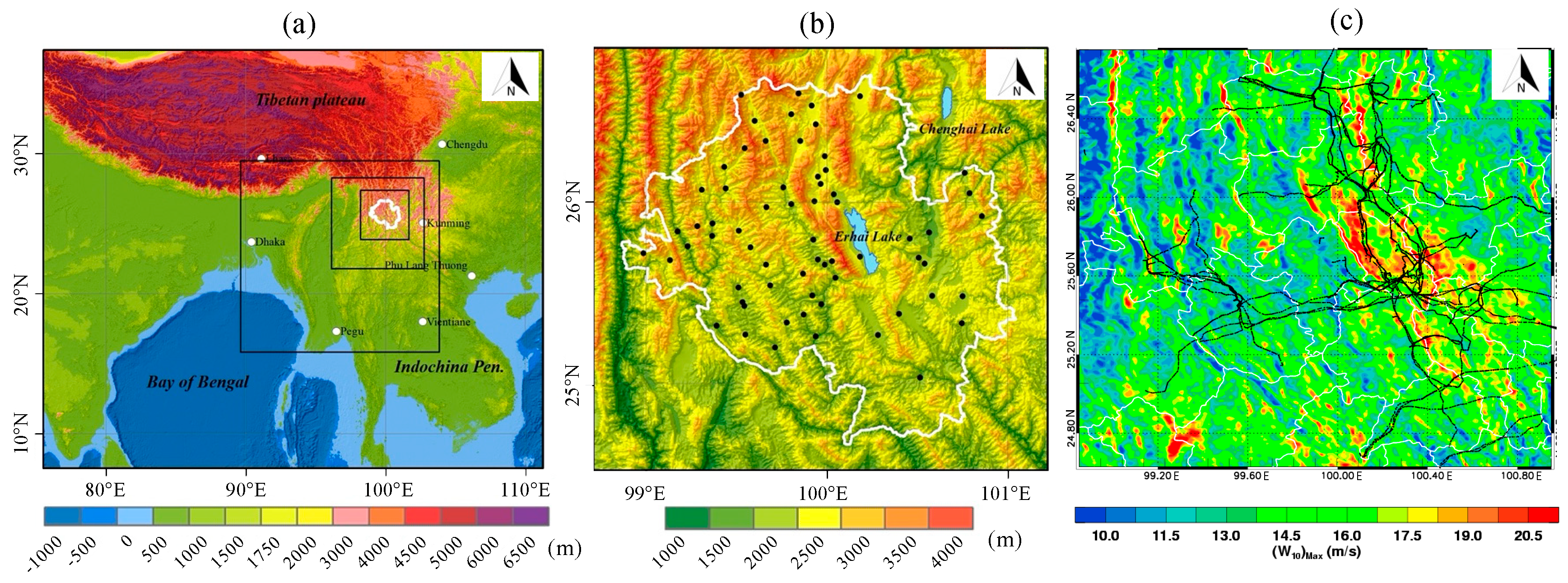
2.1. Data

Data were collected from 65 in situ stations (black dots in Figure 1b) belonging to China Meteorological Administration, from 1 January 2009 to 30 September 2017. This research selected 8 elements, namely, temperature, pressure, humidity, instantaneous wind direction, instantaneous wind velocity, 10 min average wind direction, 10 min average wind velocity, and 1 h precipitation. The distribution pattern of observation stations is inhomogeneous, with more stations in the north and fewer stations in the south, and more stations in the lower altitude region and fewer in the high-altitude region.

The initial and boundary conditions for the simulation were generated from National Centers for Environmental Prediction final analysis datasets (NCEP-FNL). The land-use types/vegetation types are from the Moderate Resolution Imaging Spectroradiometer (MODIS) classifications improved by the International Geosphere-Biosphere Program (IGBP). The terrain elevation data used in the model is the Global Multi-resolution Terrain Elevation Data (GMTED 2010), developed by the United States Geological Survey (USGS) and the National Geospatial-Intelligence Agency (NGA). In this work, 30 s high-resolution terrain data were used.

2.2. Methods

This study provides a preliminary but representative contribution to this topic by focusing on the extreme wind events detected using continuous data spanning a period of nearly 9 years. We also selected an extreme wind event as a case study to analyze the triggering of extreme wind events. First, we performed a 1-month simulation and used the observations to calibrate the parameterization schemes, and used the control model for the extreme wind simulation. Then, a series of sensitivity experiments were performed to investigate the mechanisms of extreme wind triggering, evolution, and variation, according to topography changes, land use type, soil moisture, etc. Details can be seen in the flowchart in Figure 2. Finally, we summarize the main conclusions and provide potential prospects for future research and wind disaster prevention in the context of power line installation.

2.2.1. Wind Scale Standard

The Beaufort wind scale was used in this research because it is an empirical measure that relates wind velocity to observed conditions on land and has been adopted in most areas of the world. Internationally, the World Meteorological Organization (WMO) Manual on Marine Meteorological Services defines the Beaufort wind scale up to force 12 [22]. By comparison with other wind scales, tornadoes on the Fujita and Truro wind scales lie approximately at the Beaufort number of 12 on the Beaufort wind scale [23]. This study used the thresholds method and selected one extreme wind event having a Beaufort number over 10, i.e., the wind velocity is greater than 25 m/s (

Table 1. Parts of the Beaufort Scale [22].

Beaufort Number	Wind Velocity	Land Conditions
8	39–46 mph; 62–74 km/h; 17.2–20.7 m/s	Twigs break off trees, generally impedes progress.
9	47–54 mph; 75–88 km/h; 20.8–24.4 m/s	Slight structural damage (chimney pots and slates removed).
10	55–63 mph; 89–102 km/h; 24.5–28.4 m/s	Seldom experienced inland; trees uprooted; considerable structural damage.
11	64–72 mph; 103–117 km/h; 28.5–32.6 m/s	Very rarely experienced, accompanied by widespread damage.

).

2.2.2. Statistic Methods

Two primary methods are usually used in practice for obtaining extreme wind data from a series of wind measurements: the epochal method and the peaks over thresholds method [24,25]. This research used the peaks over threshold method to define a peak value associated with each rise and fall of the measured data above the threshold.

The root means square error (RMSE) was used as a criterion for evaluating the different parameterization schemes. A smaller RMSE means a higher model performance (Equation (1)).

$$RMSE=\sqrt{\left[\frac{1}{N}{\sum }_{i=1}^N{\left(H_{i-sim}-H_{i-obs}\right)}^2\right]}$$

(1)

where RMSE is in the same units as H_i−obs and H_i−sim; i is the sampling point, H_i−obs is the actual wind velocity, H_i−sim is the simulated wind velocity, and N is the number of sampling points during the analyzed period.

2.2.3. WRF Model Set-Up and Calibrations

For near real-time prediction of the wind velocity, it is necessary to use a dynamic model such as the Weather Research and Forecasting (WRF) model or Atmosphere-Ocean General Circulation Models (AOGCMs) to simulate and to improve the prediction [26,27]. However, the real-time observation data from micro-weather stations is essential to ensure monitoring and simulation evaluation and improvements.

The WRF model is a next-generation mesoscale NWP system that can be used for operational forecasting and atmospheric research. The WRF system includes two dynamics solvers: the Advanced Research WRF (ARW) solver, which was developed primarily at NCAR, and the Nonhydrostatic Mesoscale Model solver, which was developed at NCEP. The ARW system comprises the ARW dynamics solver and additional WRF system components required to generate a simulation. WRF has many dynamical cores, a 3-Dimensional Variational (3DVar) data assimilation system, and a software architecture that enables computing parallelism and system adaptability. WRF is applicable for a wide range of scales, ranging from meters to hundreds of kilometers. Thus, WRF has been widely used in numerical weather prediction, climate downscaling simulations, air quality modeling, atmosphere–ocean interactions, idealized simulations, etc.

WRF-ARW (version 3.8.1) [28] was implemented in the present study, and was used to analyze the triggering mechanism of extreme wind events over the complex mountain area in Dali. First, we ran a simulation from 29 February to 1 April 2016 to calibrate the model configuration and physical parametrization schemes against the observations. We assessed the different initiatives and schemes of the WRF model, including 2 kinds of projections, 4 kinds of nesting domains, 5 kinds of boundary-layer schemes, with or without lake schemes, 7 kinds of microphysics schemes, 5 kinds of cumulus schemes, 4 kinds of land-surface schemes, and with or without WRF-3DVAR.

Figure 1a shows the simulated domain over Dali without and with quadruple nesting in the model configurations. The results show that both configurations can simulate topography influences on the wind distribution (Figure 1c). Overall, the maximum wind velocity is distributed along with the topography disposition, with the maximum wind velocity being concentrated over the surrounding Cangshan mountain and the Erhai lake. Compared with the one-way nesting configuration, the quadruple nesting configuration can reproduce the pattern of the maximum wind occurrences. In addition, the wind velocity from the quadruple nesting configuration is higher than that of the one-way nesting results, indicating the simulated wind velocity from the quadruple nested configuration is more consistent with the actual observations data. Furthermore, in the southwest of Dali, the quadruple nesting results show relatively larger wind velocity, especially on the top of the mountains.

The weather condition of the Dali region is mainly affected by the TP, the Yunnan-Guizhou Plateau, the South China Sea, the Bay of Bengal, and the Arabian Sea. From the observations, the prevailing wind direction in spring is southwest, indicating that the southwest monsoon coming from the Bay of Bengal and the Arabian Sea enhances the wind velocity in the region. In addition, the specific land surface, including the mountains and the Erhai lake, accelerate the wind velocity. The one-way nesting configuration may miss the influences of the large-scale meteorological background, so the simulation results are not as good as those of the quadruple nesting configuration. The outer domain (D01) in the quadruple nesting configuration covers the southwest monsoon region, which can affect the wind of the Dali region. Furthermore, the southwest monsoon can also transfer more water vapor to this area, resulting in more precipitation.

When using one-way nesting, two-way nesting, three-way nesting, and quadruple nesting configurations, the root mean square errors (RMSEs) of the one-way and two-way nesting configurations are relatively more prominent than those of the other two nesting configurations with the model running time. However, the simulation errors in the initial time for the four nesting configurations are more significant. The three-way nesting configurations were used to perform the simulations to save computing time, with the domain’s resolutions set as 1, 3, and 9 km for each domain.

To more accurately represent meteorological processes in mountain regions, the latest topography information in the WRF model derived from the United States Geological Survey/National Geospatial-Intelligence Agency Global Multi-resolution Terrain Elevation Data 2010 (USGS/NGA GMTED2010_30s) was chosen as the lower boundary conditions. In addition, considering the impact of the daily variance of lake temperature on the lake–land wind system in the innermost domain, the lake model was adopted.

We assessed different initial schemes, including different projections, boundary-layer schemes, lake schemes, microphysics schemes, cumulus schemes, land-surface schemes, and with or without WRF-3DVAR. The RMSE in different configurations is shown in Figure 3.

Based on the RMSE, we selected the following options for our control simulation (see Table 2), i.e., a Mercator projection, terrain-following coordinate, and 40 levels vertically with the top at the 50 hPa level.

The domains of control simulations (CTL) were composed of the three-nested domain centered at (23.384° N, 96.790° E), (24.850° N, 99.323° E), and (25.739° N, 100.123° E), respectively. The outermost domain (9 km grid spacing, horizontal dimension 157 × 157 grid points), the inner domain (3 km, horizontal dimension 232 × 232 grid points), and the innermost domain (1 km, horizontal dimension 313 × 313 grid points) are shown in Figure 1a. It is noted that the Betts–Miller–Janjić (BMJ) cumulus parameterization was used for the outermost domain, whereas that of the inner and innermost domains was turned off [29,30]. Other physical schemes were configured identically for all simulations with the following standard options: the Mellor–Yamada–Janjie (MYJ) boundary layer scheme [30], the NOAH land-surface model [31], the Thompson microphysics scheme [32], the Rapid Radiative Transfer Model shortwave, and the Rapid Radiative Transfer Model longwave [33] radiation schemes. In general, compared to the default simulation (Table 2), the CTL simulation can reduce the root mean square error (RMSE) of the surface wind velocity range by 1–50%.

Table 2. WRF settings for default and control simulation.

Options	Default	CTL
Shortwave radiation scheme	Dudhia [34]	RRTM
Longwave radiation scheme	RRTM	RRTM
Cumulus scheme	BMJ	BMJ
Microphysics scheme	Lin	Thompson
Planetary boundary layer scheme	YSU	MYJ
Land surface model	Noah	Noah
Lake model	Off	On
Topography information	USGS_30s	USGS/NGAGMTED2010_30s

Table 2. WRF settings for default and control simulation.

Options	Default	CTL
Shortwave radiation scheme	Dudhia [34]	RRTM
Longwave radiation scheme	RRTM	RRTM
Cumulus scheme	BMJ	BMJ
Microphysics scheme	Lin	Thompson
Planetary boundary layer scheme	YSU	MYJ
Land surface model	Noah	Noah
Lake model	Off	On
Topography information	USGS_30s	USGS/NGAGMTED2010_30s

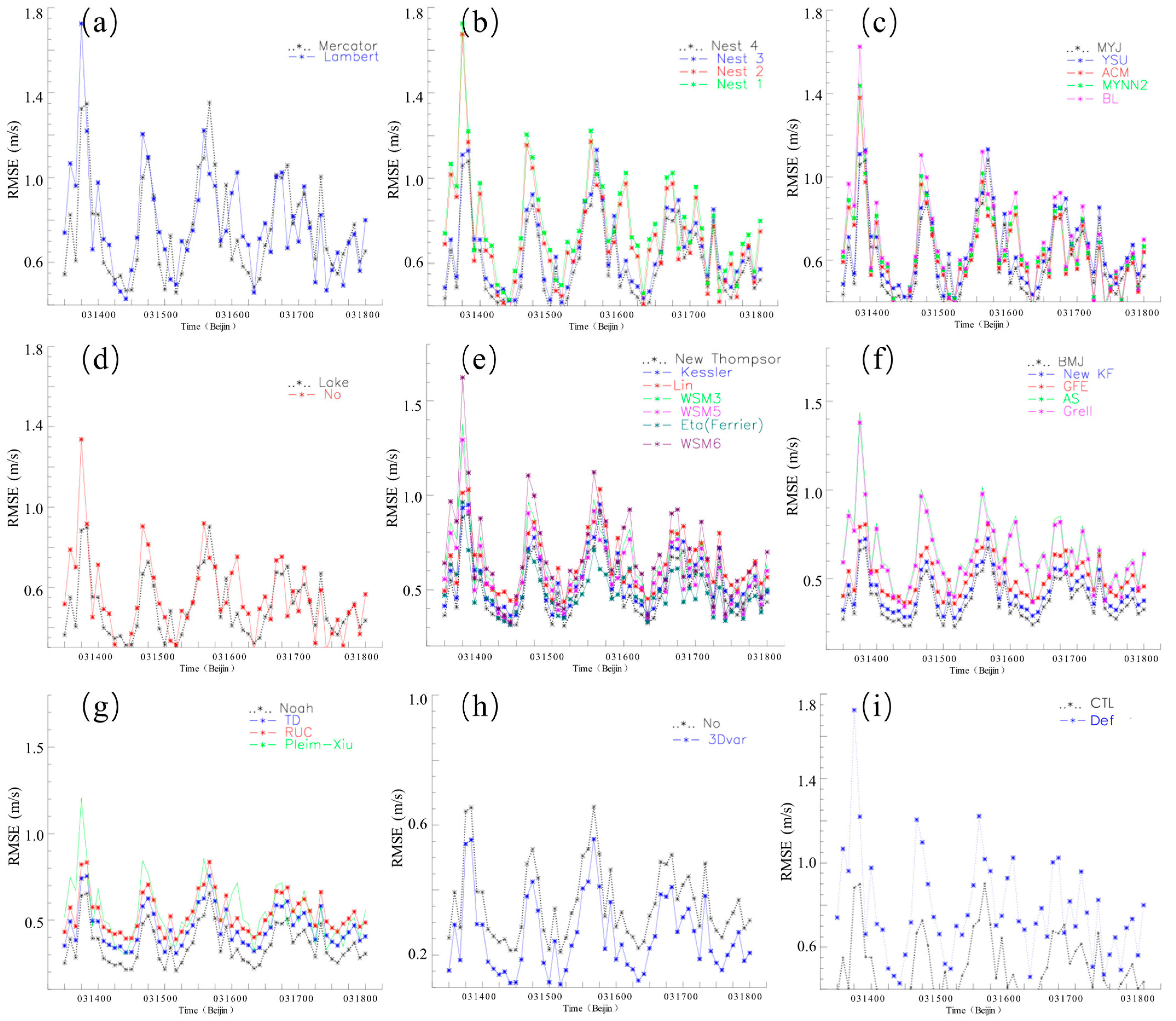
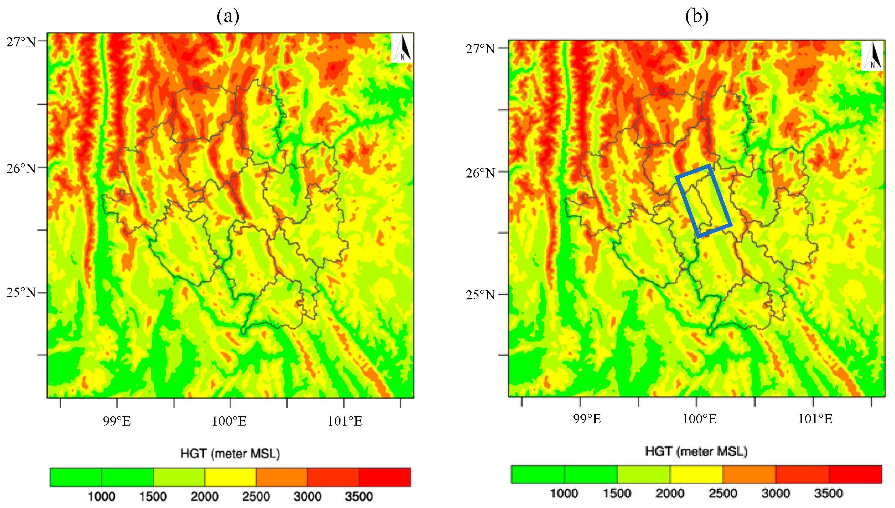
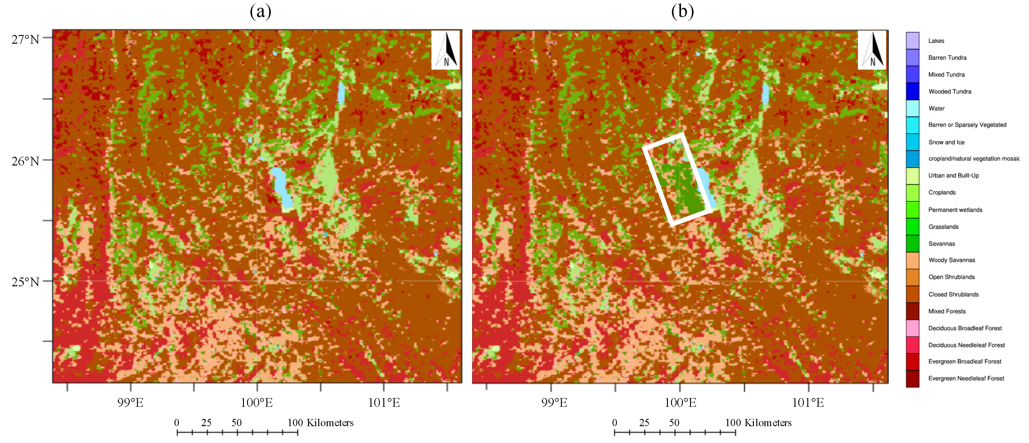
2.3. Sensitivity Experiments

This study analyzed the water–heat exchange process and its seasonal variation characteristics on the complex underlying surface and large-scale atmospheric circulation fields. Further, the formation and evolution mechanisms of near-surface wind were examined. Through the sensitivity experiments of topography, vegetation, soil moisture, and other parameters on the complex underlying surface, the influence of different factors on the extreme wind triggering process under similar surface conditions and the overlay of the large-scale circulation was studied.

Taking the extreme wind event in this region that occurred on 15 March 2016 as an example, the simulations were performed for the period 00:00 of 12 March to 18:00 of 19 March 2016 (UTC). The WRF model used a Mercator projection and terrain-following coordinates, and the model was divided vertically into 40 levels with the top at the 50 hPa level. A spin-up time of 16 h was utilized to obtain realistic initial conditions. The calibrated model simulated this strong wind event’s occurrence, development, and dissipation. A series of sensitivity tests were designed to examine the effects of different factors, such as the large-scale atmospheric circulation, the complex topography, vegetation, soil moisture, and others affecting the extreme wind event formation process (

Table 3. Sensitivity experiments.

Options	Model Default	Experiments
Nesting experiments	Same as CTL	one nested, two nested, and triple nested methods
Removing mountain	Same as CTL, one nest	Altitude over 2400 m in the Cangshan mountain modified as 2400 m
Reducing soil moisture	Same as CTL, one nest, and natural terrain	Reduce 40%
Increasing soil moisture	Same as CTL, one nest, and natural terrain	Increase 40%
Change the type of Land Use Land Cover Change (LUCC)	Same as CTL, one nest, and natural terrain	Change the land use type from forest to savanna

).

(1) Nesting experiments. Three experiments were carried out in the WRF model with one nested, two nested, and triple nested methods. Moreover, the two-way nesting method was adopted in two and triple nested experiments. By comparing the simulation results of the innermost nested region of the three experiments, the effect of the large-scale circulation of solid wind events could be ascertained.

(2) Removing mountain experiment. The high mountains with altitudes over 2400 m in the Cangshan mountains (Figure 4a) were removed and their height was modified to 2400 m (Figure 4b). This experiment was designed to analyze the influence of high mountains on wind velocity, and the initial moment of strong wind velocity formation in the mountain region.

(3) Experiment on reducing soil moisture. In this experiment, the soil moisture was reduced by 40% based on the control experiment.

(4) Experiment on increasing soil moisture. In this experiment, the soil moisture increases by 40% based on the control experiment.

(5) Experiments on the influence of vegetation type. The fractional vegetation coverage of the simulated area is higher, with that of the south being slightly higher than that of the north, and that of the west being slightly higher than that of the east. In addition, the vegetation coverage of urban and construction land areas is less than 20–30%; the fraction of mixed forest, shrubs, and savanna is 40–70%. Two lakes, named Erhai and Chenghai, are also located in the study area. In this experiment, the vegetation type in Cangshan mountain changes from forest to savanna in the WRF model (Figure 5).

3. Results

3.1. Trend of Regional Winds

We examined 9 years of wind velocity data as plotted in Figure 6 for each year. Wind velocity generally shows an annual cycle, with the smallest windspeed in August and the highest wind velocity in March; for example, the maximum wind velocity in this region in the past 9 years was 28 m/s in March. The southerly wind prevails throughout the year, with an average wind direction of 201 degrees southwest; winds below scale 5 prevail throughout the year; the maximum wind velocity is 9 scale; and occasionally 10-scale wind occurs.

By analyzing the observation data, the diurnal variation in wind velocity in this region is in the form of a single peak. The wind velocity is low at night and gradually increases during the day, and the maximum wind velocity is typically reached in the afternoon.

3.2. Local Micro-Meteorological Conditions

Figure 7 shows wind velocity and direction distribution, air temperature, and relative humidity at 2 m at 07:00 UTC on 15 March 2016. The direction of the 10-scale wind is west, with the maximum wind center located at the top of the mountain on the windward slope. Moreover, the 10-scale wind occurred in the minimum air temperature region and the area of maximum relative humidity, which reached more than 75%. This partly demonstrates that the maximum wind may be triggered by both the large-scale circulation and the local micro-meteorological conditions.

3.3. The Triggering Mechanism

Three sensitivity experiments were performed to simulate the wind on 15 March (Figure 8). The 8-scale wind occurred at 06:00 UTC for the one-way nesting configuration and continued for 4 h until 10:00 UTC. The strong wind concentrated over the region with the maximum altitude. Furthermore, the wind directions were mainly west and southwest. For the two-way nesting configuration, as in the one-way nesting, the 8-scale wind occurred at 06:00 UTC, whereas the wind velocity at 07:00 UTC reached 10-scale and 11-scale, and wind stronger than scale 10 continued for 3 h. This indicates that the local conditions can trigger an 8-scale wind, where the scale 10- and 11-level winds are mainly triggered by both the topography and the large-scale circulation. For the three-nesting configurations, the 10-scale wind was generated at 06:00 UTC, which was 1 h earlier than the two-way nesting configuration, and reached scale 11 at 07:00 UTC. Winds of scale 10 and above continued for 2 h. From these sensitivity experiments, we can conclude that local geographic conditions generate winds of scale 8 and below, where 10- and 11-scale winds are triggered by both the local geographic conditions and the large-scale circulations coming from the west and the southwest regions, including the Hengduan mountain, Yunnan-Guizhou Plateau, and the Bay of Bengal. According to the observations of the Dali Meteorological Administration, the 10-scale wind was captured at 14:00 UTC, which is consistent with the simulation of the three-nesting configuration, further demonstrating that wind of scale 10 and above is triggered by the passing of the vital weather processes from the southwest Bay of Bengal. This, the strong wind of scale 10 and above is triggered by the joint influences of local geographic conditions and the large-scale background, resulting in the wind that caused damage to transmission lines. Because the domains of the two-nesting and three-nesting configurations are relatively more extensive than that of the one-way nesting configuration, which introduces the influences of the large-scale circulation, we selected the one-way nesting configuration to perform the sensitivity experiments on local conditions triggering the wind in the case of the impact of the large-scale circulation.

When the mountain was removed in the sensitivity experiment, the wind velocity change to scale 4 compared with the 8- to 9-scale wind in the control experiment. In addition, no wind stronger than scale 4 occurred in the experiment in which the mountain was removed, indicating the mountain topography is a vital factor for triggering the 8- to 9-scale wind. As a result, without considering the influence of the large-scale circulation, wind of scale 8 and below is mainly triggered by local geographic conditions.

When we changed the vegetation of the Cangshan mountain, where the 8- to 9-scale wind occurred, from forest to savanna, it was found that the wind scale was similar to that of the control experiment, but the wind velocity was accelerated and the area was also slightly increased. The existence of the forest may reduce the wind velocity, but only to a small extent.

When soil moisture of the simulated region was increased by 40% compared to the control value, the maximum wind scale was reduced by 1 scale, with the maximum wind velocity occurring at the same time as that of the control experiment. Compared with the sensitivity experiment in which soil moisture was reduced by 40%, the experiment in which soil moisture was increased showed that the maximum wind occurred at 08:00 UTC, which was 2 h earlier than in the experiment in which soil moisture was reduced. This indicates a change in soil moisture of 40% can affect the scale of the wind, and increasing soil moisture can increase the area in which strong wind occurs.

4. Discussion

As noted in the work of Bastine et al. [21], reliable estimates of extreme winds are crucial, and are a challenge for wind energy and power line design. However, local adopted parameters or related schemes are difficult to derive due to a lack of field observations, including observations of the distribution of surface roughness, and thermal and dynamic roughness length. In addition, to ensure numerical stability, smoothing is embedded in mesoscale simulations, which reduces variability in the wind and consequently leads to an underestimation of maximum wind speeds.

In addition, the mechanisms that trigger maximum wind speeds also differ due to the atmospheric background and effective local factors. Based on the results of five sensitivity experiments, the calibrated WRF model suggested that the high mountain is a crucial factor in the formulation of the extreme wind velocity. The increase or decrease in soil moisture can reduce the wind energy scale by 40%. A 40% increase in soil moisture can also advance the appearance of extreme wind areas by 2 h. If the vegetation type is changed from forest to prairie, the wind scale remains the same; however, the wind velocity value increases slightly and the range of the extreme wind area also increases. Although forests can weaken the wind energy, the degree of weakening does not exceed 1 scale.

As shown in Figure 1, a portion of the power lines is distributed in areas experiencing maximum wind speeds, especially in the mountain edges to the west and east of Erhai Lake, which enhances the risk of wind damage to these lines. For the existing power lines, it is essential to establish protection and warning solutions for safe operation. Furthermore, it is necessary to avoid regions in which maximum wind speeds occur when designing new power lines or adding more connectors. In the near future, it will be necessary to integrate the mesoscale WRF model with a microscale model for wind velocity simulation. In particular, the dynamic and thermal processes at the large scale, mesoscale, and microscale can be taken into account. Thus, a better description of the local terrain effect up to the maximum extreme wind extent can be expected to provide improved simulations.

5. Conclusions

By comparing the observations and performing sensitivity experiments using the WRF model of extreme wind over the complex mountain area in the Dali region in the Yunnan-Guizhou Plateau in China, we obtained the following conclusions.

(1)

Using a three-nesting domain with the MODIS land-use type, MYJ boundary layer scheme, the NOAH land-surface model, the Thompson microphysics scheme, and the RRTM shortwave and longwave radiation schemes, with 30 s high-resolution terrain datasets, the RMSE of the simulated wind velocity can be reduced by more than 50%.

(2)

In this study, we identified a powerful wind mechanism in regions having a high altitude and continuous topography, in which the terrain uplift has the most significant impact on the occurrence of local 8–9-scale extreme winds. When a large-scale atmospheric circulation is passing, accompanied with regional terrain lifting, the instantaneous wind velocity can reach the scale of 9 to 10 ( mean wind velocity between 20.8 and 28.4 m/s), causing damage to power lines.

(3)

Lifting due to high and concentrated mountains plays an import role in the triggering of 8- to 9-scale winds. In addition, wind is accelerated due to the passing of large-scale processes, which results in damage to transmission lines. Other factors, such as surface soil moisture and the land surface, including changing the forest to savanna, can affect the velocity and extent of the wind, but these influences can be limited. Both soil moisture and land use type can affect energy and water transfer between the land surface and the atmosphere. Local dry and wet conditions, particularly relating to soil moisture, influence the atmosphere via a feedback mechanism, and thus have a joint effect on the possible destructive effects of the wind on transmission lines. Therefore, when establishing transmission lines, it is vital to avoid sites where these factors may play an influencing role.

References

1. Zhang, S.; Solari, G.; Yang, Q.; Repetto, M.P. Extreme wind speed distribution in a mixed wind climate. J. Wind. Eng. Ind. Aerodyn. 2018, 176, 239–253. [Google Scholar] [CrossRef]
2. Waliser, D.; Guan, B. Extreme winds and precipitation during landfall of atmospheric rivers. Nat. Geosci. 2017, 10, 179–183. [Google Scholar] [CrossRef]
3. Gomes, L.; Vickery, B.J. Extreme wind speeds in mixed climates. J. Ind. Aerod. 1978, 2, 331–344. [Google Scholar] [CrossRef]
4. Marchigiani, R.; Gordy, S.; Cipolla, J.; Adams, R.C.; Evans, D.C.; Stehly, C.; Galwankar, S.; Russell, S.; Marco, A.P.; Kman, N.; et al. Wind disasters: A comprehensive review of current management strategies. Int. J. Crit. Illn. Inj. Sci. 2013, 3, 130–142. [Google Scholar] [PubMed]
5. Zhang, Y.; Lam, J.S.L. Estimating the economic losses of port disruption due to extreme wind events. Ocean. Coast. Manag. 2015, 116, 300–310. [Google Scholar] [CrossRef]
6. Wang, C.-H.; Wang, X.; Khoo, Y.B. Extreme wind gust hazard in Australia and its sensitivity to climate change. Nat. Hazards 2013, 67, 549–567. [Google Scholar] [CrossRef]
7. Britannica, T.E.O.E. Wind. Encyclopedia Britannica, 2020. Available online: https://www.britannica.com/science/wind (accessed on 8 January 2022).
8. Löffler, J.; Anschlag, K.; Baker, B.; Finch, O.-D.; Wundram, D.; Diekkrüger, B.; Schröder, B.; Pape, R.; Lundberg, A. Mountain ecosystem response to global change. Erdkunde 2011, 6, 189–213. [Google Scholar] [CrossRef] [Green Version]
9. Deng, W.; Cheng, G.; Wen, A. The conception of mountain science development in China. Discip. Dev. 2008, 23, 156–161. [Google Scholar]
10. Mo, H.M.; Hong, H.P.; Fan, F. Estimating the extreme wind speed for regions in China using surface wind observations and reanalysis data. J. Wind. Eng. Ind. Aerodyn. 2015, 143, 19–33. [Google Scholar] [CrossRef]
11. Huicong, J.; Pan, D.; Wang, J.-A.; Zhang, W.-C. Risk mapping of integrated natural disasters in China. Nat. Hazards 2016, 80, 2023–2035. [Google Scholar]
12. Dearing, J.A.; Jones, R.T.; Shen, J.; Yang, X.; Boyle, J.F.; Foster, G.C.; Crook, D.S.; Elvin, M.J.D. Using multiple archives to understand past and present climate–human–environment interactions: The lake Erhai catchment, Yunnan Province, China. J. Paleolimnol. 2008, 40, 3–31. [Google Scholar] [CrossRef]
13. Li, B.; Morton, L.C.; Liu, Q. Climate change and mosquito-borne diseases in China: A review. Glob. Health 2013, 9, 10. [Google Scholar]
14. Dai, J.; Tan, Y.; Yang, W.; Wen, L.; Shen, X. Investigation of wind resource characteristics in mountain wind farm using multiple-unit SCADA data in Chenzhou: A case study. Energy Convers. Manag. 2017, 148, 378–393. [Google Scholar] [CrossRef] [Green Version]
15. Ohata, T.; Higuchi, K.; Ikegami, K. Mountain-valley wind system in the Khumbu Himal, East Nepal. J. Meteorol. Soc. Jpn. Ser. II 1981, 59, 753–762. [Google Scholar] [CrossRef] [Green Version]
16. Bert, B.; Hooff, T.v.; Aanen, L.; Bronsema, B. Computational analysis of the performance of a venturi-shaped roof for natural ventilation: Venturi-effect versus wind-blocking effect. Comput. Fluids 2011, 48, 202–213. [Google Scholar]
17. Wei, C.; Zhong, S.; Geng, Y.; Chen, Y.; Cui, X.; Wu, Q.; Pan, H.; Wu, R.; Sun, L.; Tian, X. Emergy based sustainability evaluation for Yunnan Province, China. J. Clean. Prod. 2017, 162, 1388–1397. [Google Scholar]
18. Fu, X.; Wang, J.; Li, H.-N.; Li, J.-X.; Yang, L.-D. Full-scale test and its numerical simulation of a transmission tower under extreme wind loads. J. Wind. Eng. Ind. Aerodyn. 2019, 190, 119–133. [Google Scholar] [CrossRef]
19. Lin, J.; Sun, Y.-Z.; Cheng, L.; Gao, W.-Z. Assessment of the power reduction of wind farms under extreme wind condition by a high resolution simulation model. Appl. Energy 2012, 96, 21–32. [Google Scholar] [CrossRef]
20. Lin, N.; Smith, J.A.; Villarini, G.; Marchok, T.P.; Baeck, M.L. Modeling Extreme Rainfall, Winds, and Surge from Hurricane Isabel (2003). Weather Forecast. 2010, 25, 1342–1361. [Google Scholar] [CrossRef]
21. Bastine, D.; Larsén, X.; Witha, B.; Dörenkämper, M.; Gottschall, J. Extreme Winds in the New European Wind Atlas. J. Phys. Conf. Ser. 2018, 1102, 012006. [Google Scholar] [CrossRef]
22. World Meteorological Organization. Manual on Marine Meteorological Services: Volume I–Global Aspect; World Meteorological Organization: Geneva, Switzerland, 2012. [Google Scholar]
23. Edwards, R.; LaDue, J.G.; Ferree, J.T.; Scharfenberg, K.; Maier, C.; Coulbourne, W.L. Tornado intensity estimation: Past, present, and future. BAMS 2013, 94, 641–653. [Google Scholar] [CrossRef]
24. Vinoth, J.; Young, I.R. Global Estimates of Extreme Wind Speed and Wave Height. J. Clim. 2011, 24, 1647–1665. [Google Scholar] [CrossRef]
25. An, Y.; Pandey, M.D. A comparison of methods of extreme wind speed estimation. J. Wind. Eng. Ind. Aerodyn. 2005, 93, 535–545. [Google Scholar] [CrossRef]
26. Martins, J.; Rocha, A.; Viceto, C.; Pereira, S.C.; Santos, J.A. Future Projections for Wind, Wind Shear and Helicity in the Iberian Peninsula. Atmosphere 2020, 11, 1001. [Google Scholar] [CrossRef]
27. Luca, P.D.; Harpham, C.; Wilby, R.L.; Hillier, J.K.; Franzke, C.L.E.; Leckebusch, G.C. Past and Projected Weather Pattern Persistence with Associated Multi-Hazards in the British Isles. Atmosphere 2019, 10, 577. [Google Scholar] [CrossRef] [Green Version]
28. Skamarock, W.C.; Klemp, J.B. A time-split nonhydrostatic atmospheric model for weather research and forecasting applications. J. Comput. Phys. 2008, 227, 3465–3485. [Google Scholar] [CrossRef]
29. Betts, A.; Miller, M. A new convective adjustment scheme. Part II: Single column tests using GATE wave, BOMEX, ATEX and arctic air-mass data sets. Q. J. R. Meteorol. Soc. 1986, 112, 693–709. [Google Scholar]
30. Janjić, Z.I. The step-mountain eta coordinate model: Further developments of the convection, viscous sublayer, and turbulence closure schemes. Mon. Weather. Rev. 1994, 122, 927–945. [Google Scholar] [CrossRef] [Green Version]
31. Chen, F.; Dudhia, J. Coupling an advanced land surface–hydrology model with the Penn State–NCAR MM5 modeling system. Part I: Model implementation and sensitivity. Mon. Weather. Rev. 2001, 129, 569–585. [Google Scholar] [CrossRef] [Green Version]
32. Thompson, G.; Field, P.R.; Rasmussen, R.M.; Hall, W.D. Explicit forecasts of winter precipitation using an improved bulk microphysics scheme. Part II: Implementation of a new snow parameterization. Mon. Weather. Rev. 2008, 136, 5095–5115. [Google Scholar] [CrossRef]
33. Mlawer, E.J.; Taubman, S.J.; Brown, P.D.; Iacono, M.J.; Clough, S.A. Radiative transfer for inhomogeneous atmospheres: RRTM, a validated correlated-k model for the longwave. J. Geophys. Res. Atmos. 1997, 102, 16663–16682. [Google Scholar] [CrossRef] [Green Version]
34. Dudhia, J. Numerical study of convection observed during the winter monsoon experiment using a mesoscale two-dimensional model. J. Atmos. Sci. 1989, 46, 3077–3107. [Google Scholar] [CrossRef]
Figure 1. Research region and the extreme wind distribution: (a) the three-nested domain (black squares) of simulations overlaid with the topography (shade, m) of the study area (white line); (b) meteorological stations (black dots); (c) distribution of simulated maximum instantaneous wind velocity and locations of power lines (black lines) in the Dali region.
Atmosphere 13 00133 g001
Figure 2. Flowchart of the extreme wind triggering mechanism investigation.
Atmosphere 13 00133 g002
Figure 3. RMSE of simulated wind velocity from different initial and physical parameterization schemes using the WRF model against observations: (a) Lambert (blue star line) and Mercator (black dot line) projection; (b) different nesting; (c) 5 kinds of boundary-layer schemes; (d) with and without lake scheme; (e) 7 kinds of microphysics schemes; (f) 5 kinds of cumulus schemes; (g) 4 kinds of land-surface schemes; (h) with and without WRF-3DVAR; (i) default (star and blue line) and CTL simulation (black dot line).
Atmosphere 13 00133 g003
Figure 4. Altitude distribution of the topography experiments: (a) CTL; (b) with the mountain in the blue rectangle removed.
Atmosphere 13 00133 g004
Figure 5. Land-use type distribution of the sensitive experiments: (a) CTL; (b) with the land use over the surrounding mountain area changed from forest to savanna.
Atmosphere 13 00133 g005
Figure 6. (a) Wind velocity boxplot in each month in the Dali region for 9 years (2009–2017) based on in situ observations from 65 sites (the black stars indicate cases in which wind velocity was over 24 m/s). (b) Daily wind velocity from 13 to 20 March 2016 (black stars show national stations, red circles show local stations).
Atmosphere 13 00133 g006
Figure 7. Wind velocity and direction (left), with shading produced by a digital elevation model (DEM), air temperature (middle), and relative humidity (right) at 2 m at 07:00 UTC on 15 March. The wind barb indicates the wind direction (the top of the staff shows the direction from which the wind is coming) and wind speed (indicated by feathers added to the top of the staff, with a short feather representing a 5 mph average wind speed and a long feather equal to 10 mph).
Atmosphere 13 00133 g007
Figure 8. Simulated wind vector and digital elevation model in the innermost WRF model domain on 15 Marth 2016. Shaded was produced by a digital elevation model (DEM). The wind barb indicates the wind direction (the top of the staff shows the direction from which the wind is coming) and wind speed (indicated by feathers added to the top of the staff, with a short feather representing a 5 mph average wind speed and a long feather equal to 10 mph): (a) atmospheric circulation (nesting experiment), (b) removing the mountain, (c) changing the type of vegetation from forest to savanna.
Atmosphere 13 00133 g008