
Combining vLAPS and Nudging Data Assimilation

 ,
,  ,
,
Abstract
1. Introduction
2. Materials and Methods
2.1. WRF-ARW
2.2. vLAPS
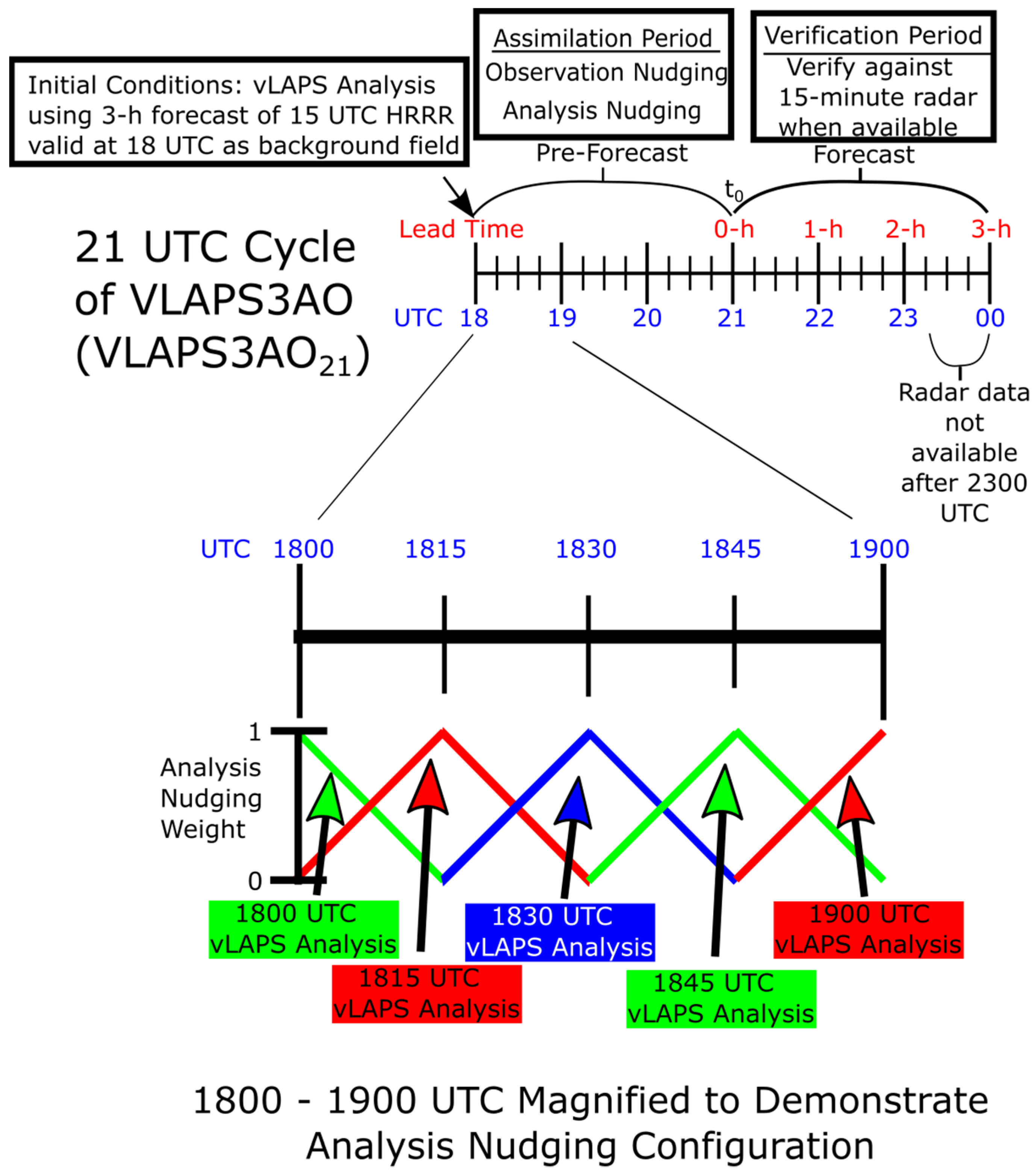
2.3. Nudging
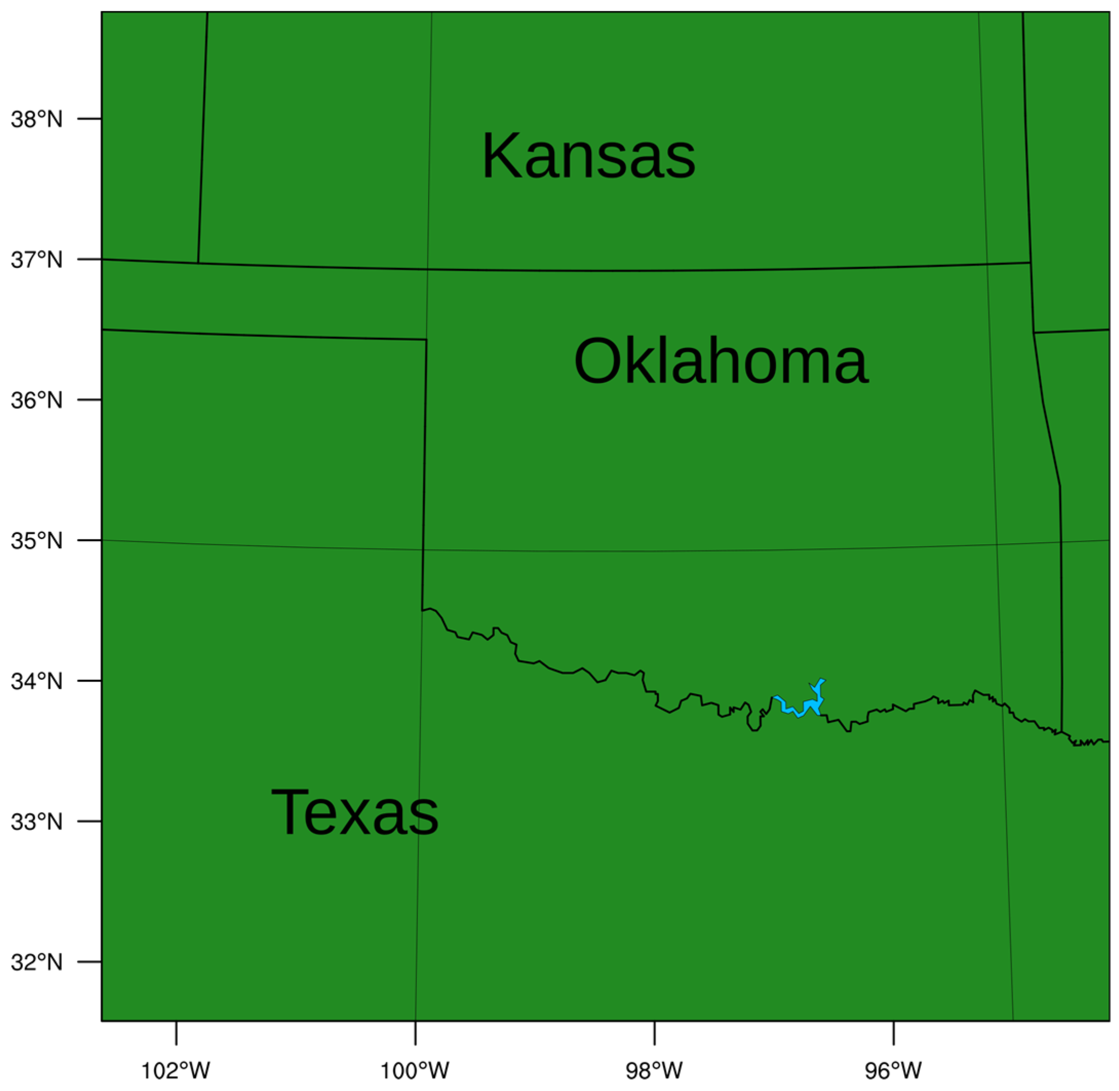
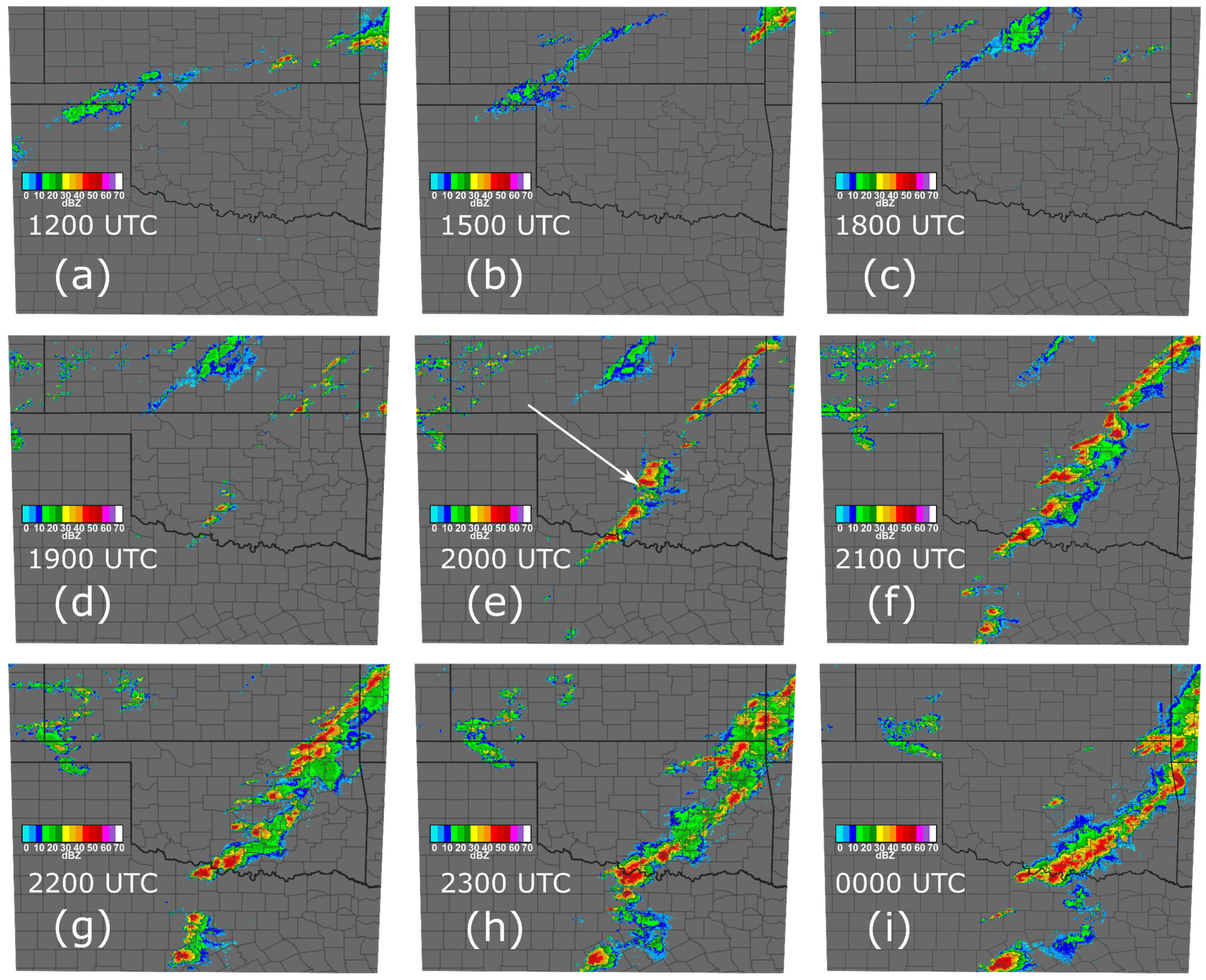
2.4. Case Description
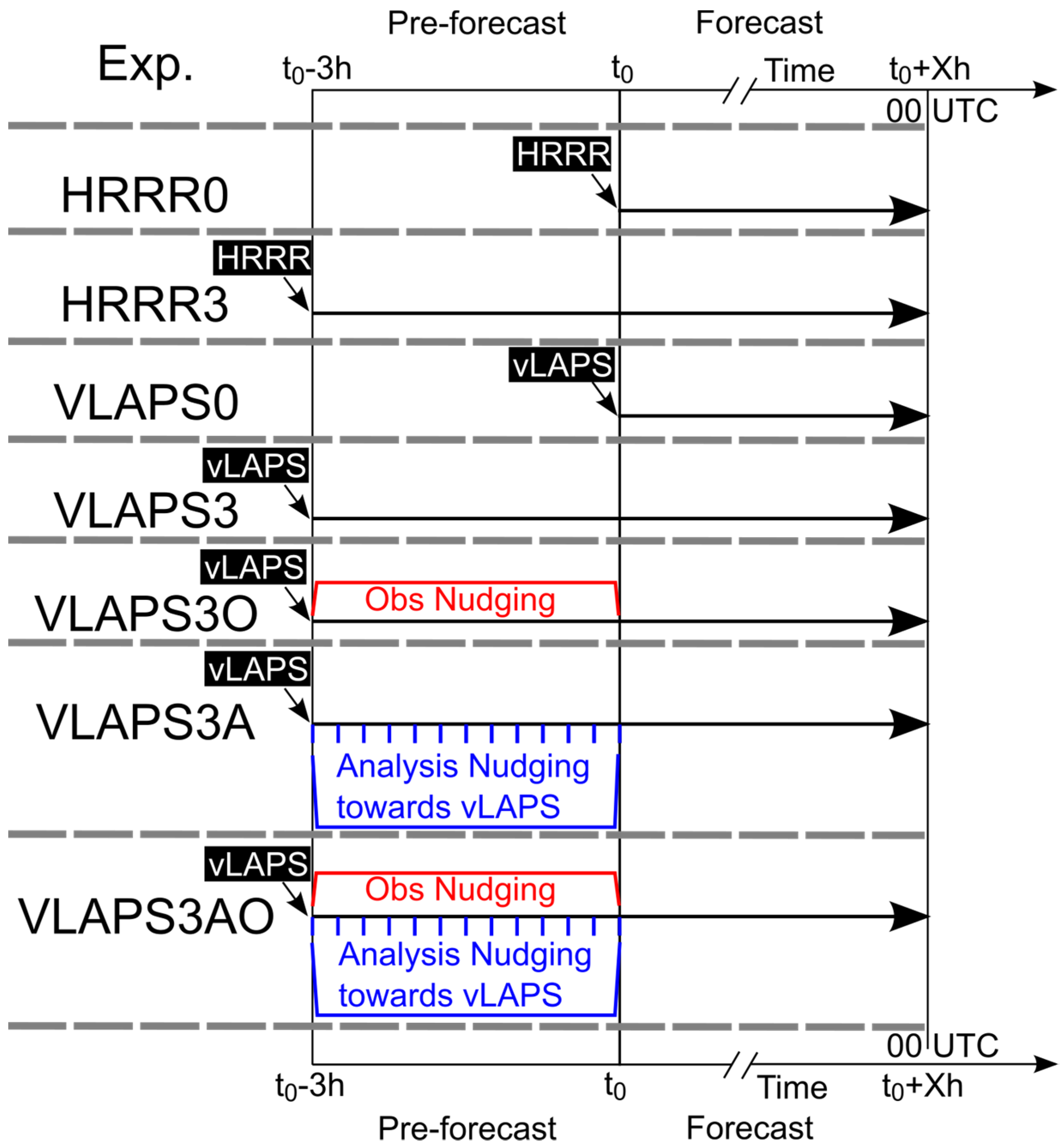
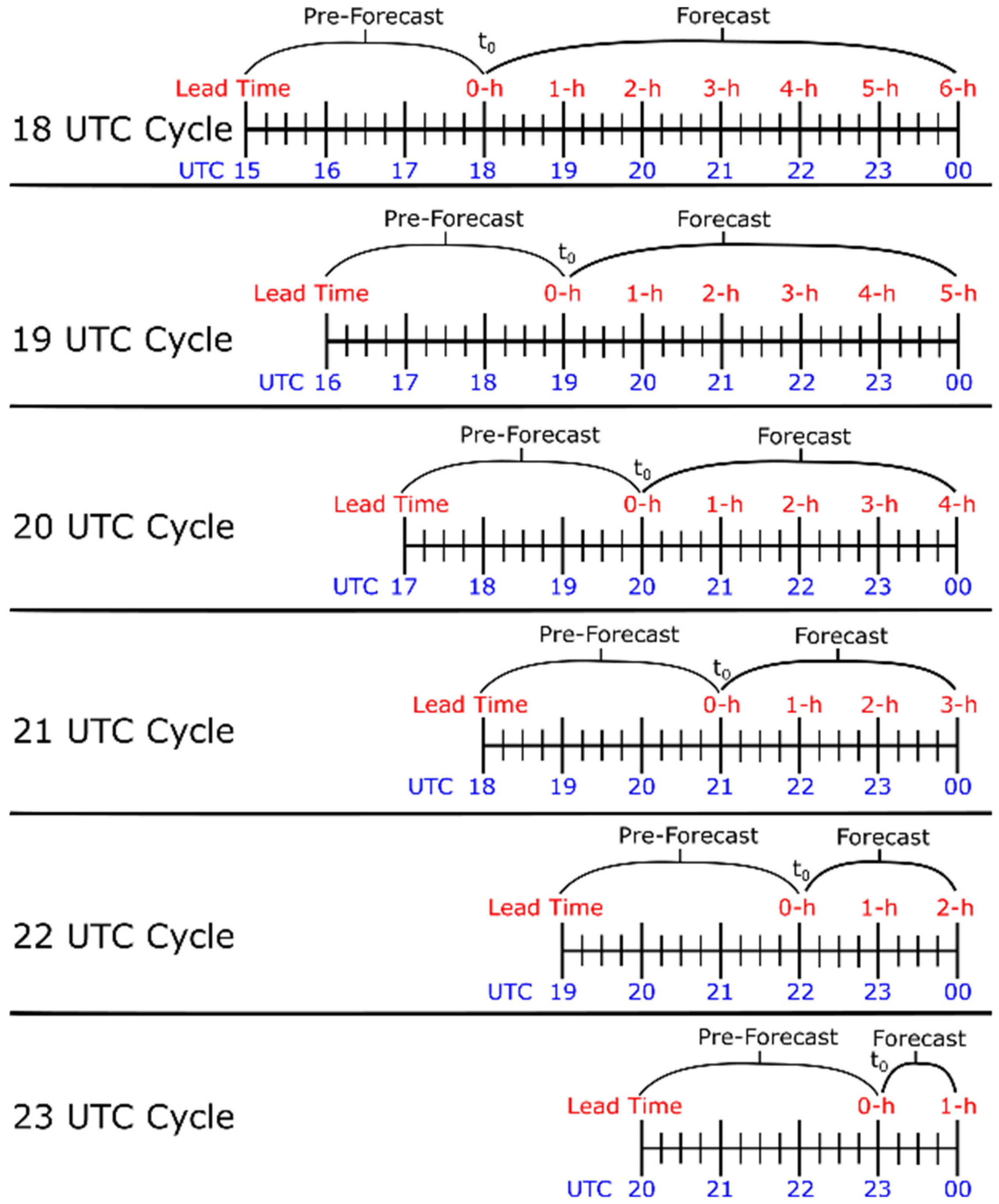
2.5. Experiment Design
3. Results
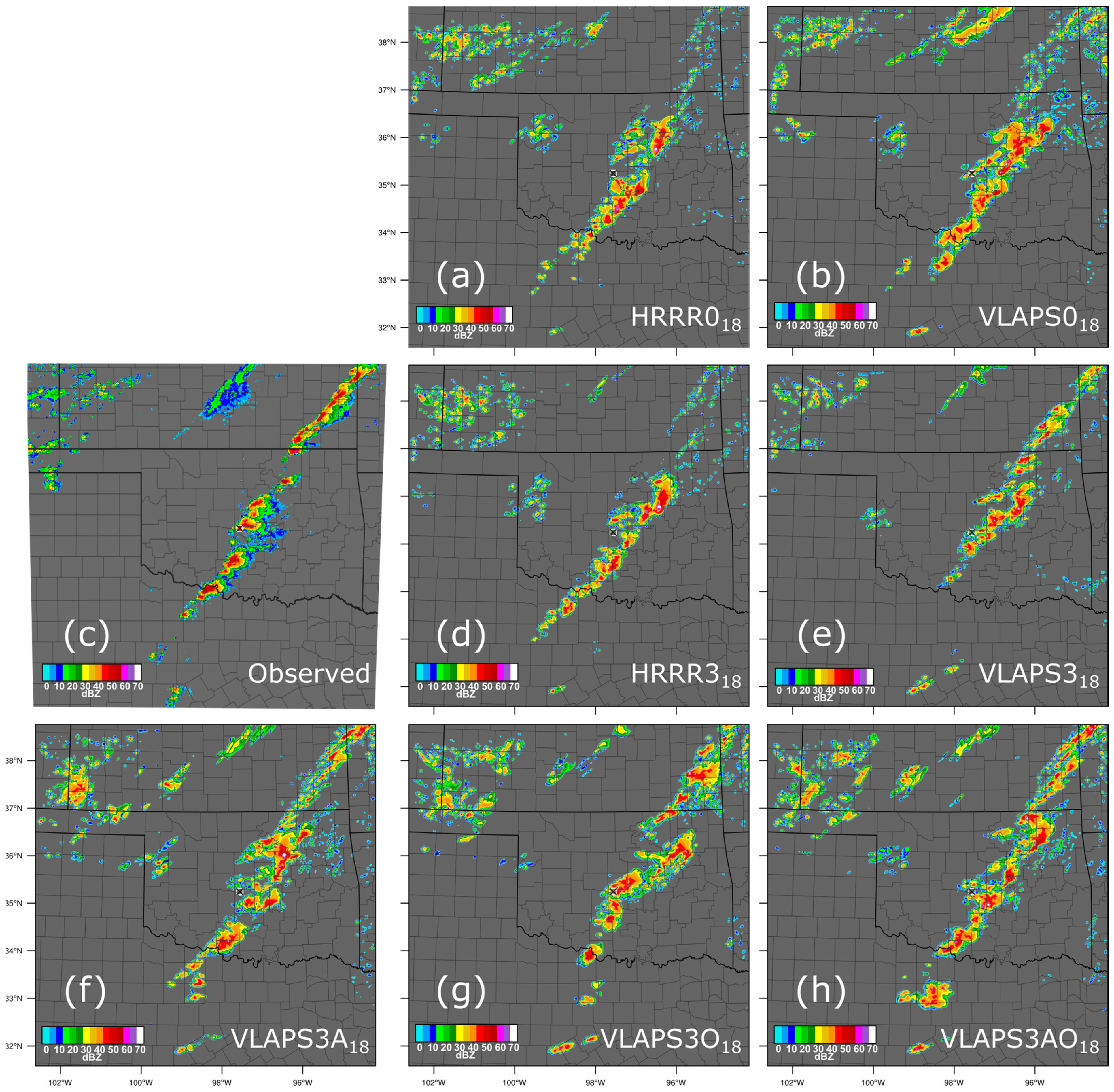
3.1. Subjective Evaluation
3.2. Objective Evaluation
3.2.1. Metrics Used in Objective Evaluation
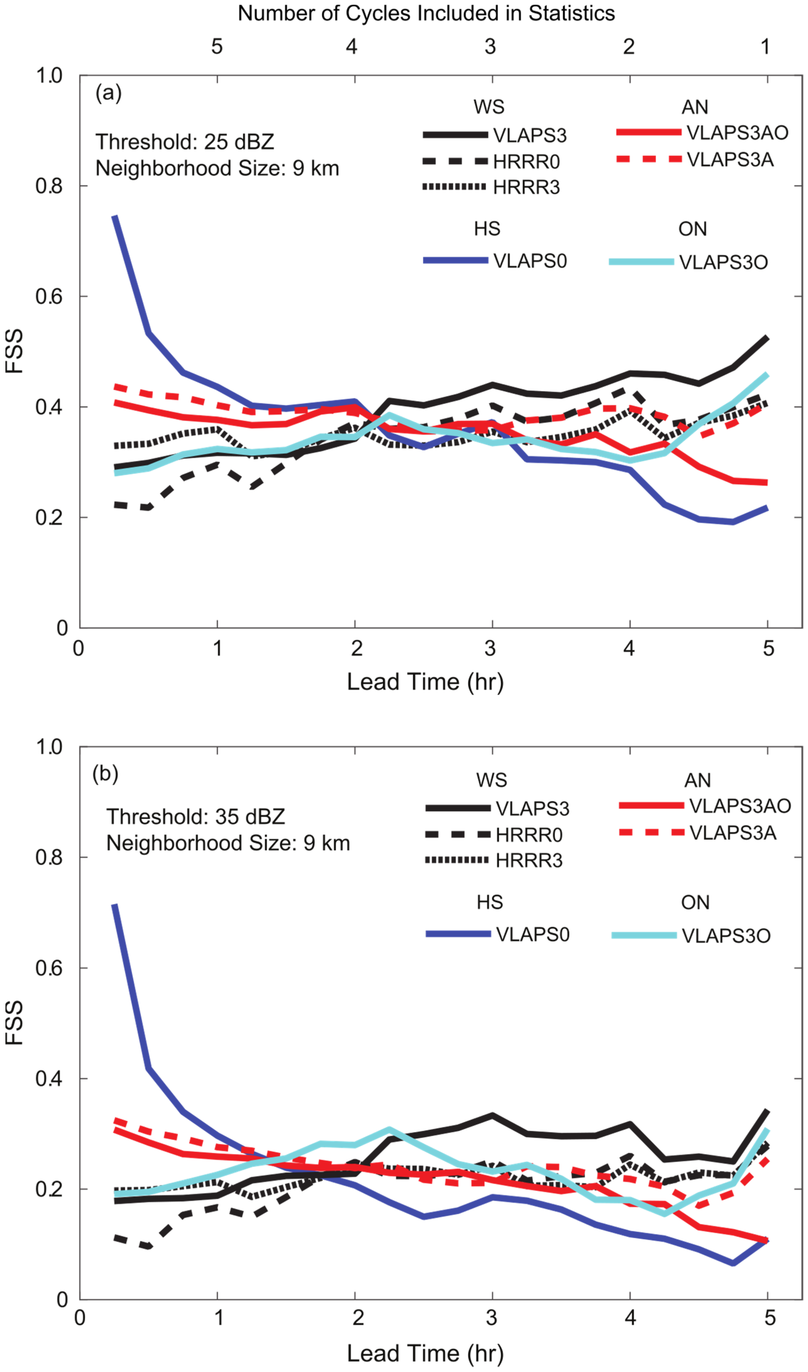
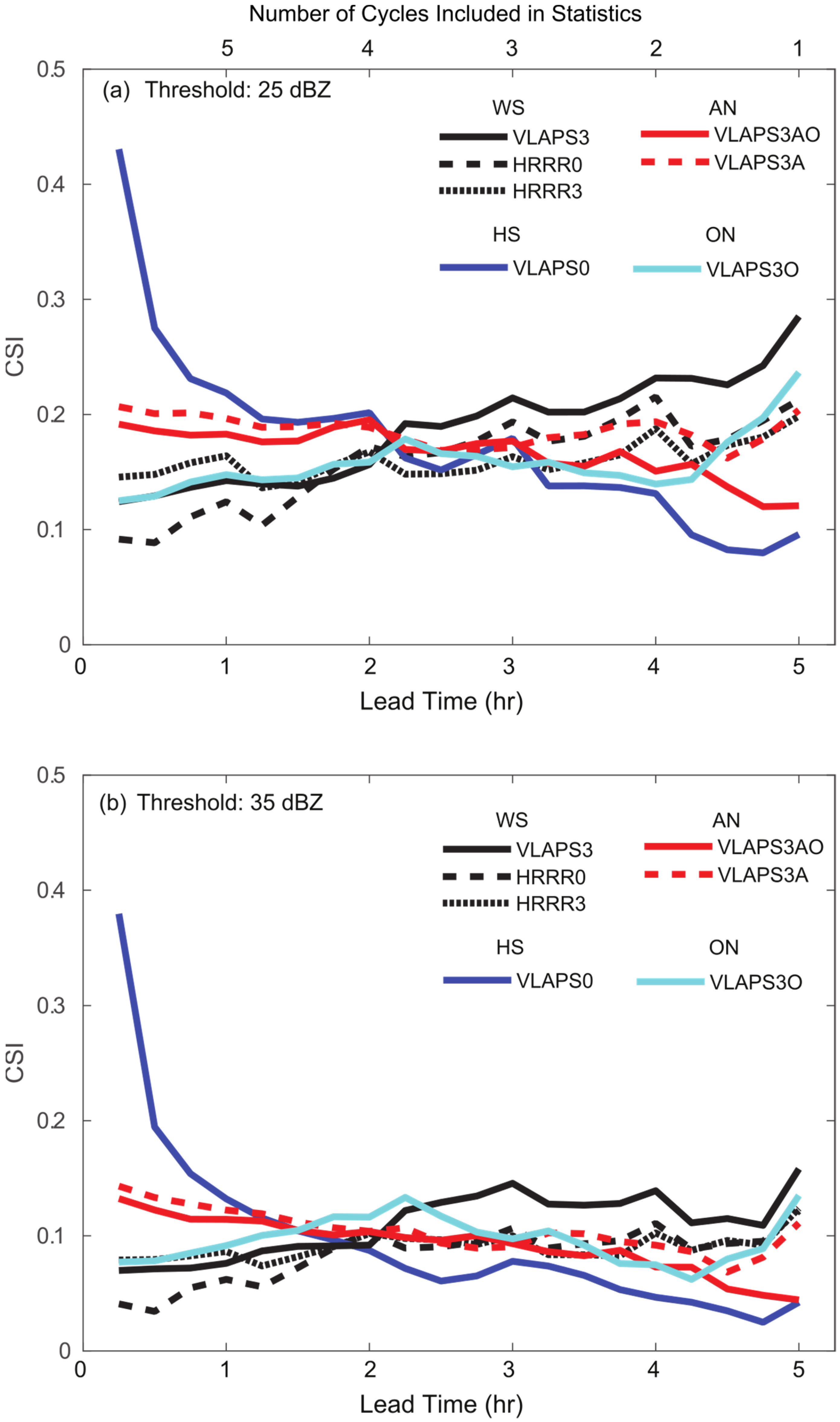
3.2.2. Outcome of Objective Evaluation
4. Discussion
Author Contributions
Funding
Data Availability Statement
Acknowledgments
Conflicts of Interest
References
- Hu, M.; Xue, M.; Brewster, K. 3DVAR and Cloud Analysis with WSR-88D Level-II Data for the Prediction of the Fort Worth, Texas, Tornadic Thunderstorms. Part I: Cloud Analysis and Its Impact. Mon. Weather Rev. 2006, 134, 675–698. [Google Scholar] [CrossRef]
- Xiao, Q.; Sun, J. Multiple-Radar Data Assimilation and Short-Range Quantitative Precipitation Forecasting of a Squall Line Observed during IHOP_2002. Mon. Weather Rev. 2007, 135, 3381–3404. [Google Scholar] [CrossRef]
- Schroeder, A.J.; Stauffer, D.R.; Seaman, N.L.; Deng, A.; Gibbs, A.M.; Hunter, G.K.; Young, G.S. An Automated High-Resolution, Rapidly Relocatable Meteorological Nowcasting and Prediction System. Mon. Weather Rev. 2006, 134, 1237–1265. [Google Scholar] [CrossRef]
- Reen, B.P.; Stauffer, D.R. Data assimilation strategies in the planetary boundary layer. Bound.-Layer Meteorol. 2010, 137, 237–269. [Google Scholar] [CrossRef]
- Hu, M.; Benjamin, S.G.; Ladwig, T.T.; Dowell, D.C.; Weygandt, S.S.; Alexander, C.R.; Whitaker, J.S. GSI Three-Dimensional Ensemble–Variational Hybrid Data Assimilation Using a Global Ensemble for the Regional Rapid Refresh Model. Mon. Weather Rev. 2017, 145, 4205–4225. [Google Scholar] [CrossRef]
- Lee, M.; Kuo, Y.; Barker, D.M.; Lim, E. Incremental Analysis Updates Initialization Technique Applied to 10-km MM5 and MM5 3DVAR. Mon. Weather Rev. 2006, 134, 1389–1404. [Google Scholar] [CrossRef]
- Brewster, K.A.; Stratman, D.R. Tuning an analysis and incremental analysis updating assimilation for an efficient high-resolution forecast system. In Proceedings of the 20th Conference on Integrated Observing and Assimilation Systems for the Atmosphere, Oceans and Land Surface (IAOS-AOLS), New Orleans, LA, USA, 11–14 January 2016; Available online: https://ams.confex.com/ams/96Annual/webprogram/Paper289235.html (accessed on 10 November 2021).
- Lorenc, A.C.; Rawlins, F. Why does 4D-Var beat 3D-Var? Quart. J. Roy. Meteor. Soc. 2005, 131, 3247–3257. [Google Scholar] [CrossRef]
- Stauffer, D.R.; Seaman, N.L. Use of Four-Dimensional Data Assimilation in a Limited-Area Mesoscale Model. Part I: Experiments with Synoptic-Scale Data. Mon. Weather Rev. 1990, 118, 1250–1277. [Google Scholar] [CrossRef]
- Stauffer, D.R.; Seaman, N.L.; Binkowski, F.S. Use of Four-Dimensional Data Assimilation in a Limited-Area Mesoscale Model Part II: Effects of Data Assimilation within the Planetary Boundary Layer. Mon. Weather Rev. 1991, 119, 734–754. [Google Scholar] [CrossRef]
- Shaw, B.L.; Carpenter, R.L.; Spencer, P.L.; DuFran, Z. Commercial Implementation of WRF with Efficient Computing and Advanced Data Assimilation. In Proceedings of the 9th Annual WRF User’s Workshop, Boulder, CO, USA, 23–27 June 2008; Available online: http://www2.mmm.ucar.edu/wrf/users/workshops/WS2008/abstracts/2-05.pdf (accessed on 10 November 2021).
- Liu, Y.; Yu, W.; Warner, T.; Sun, J.; Xiao, Q.; Pace, J. Short-term explicit forecasting and nowcasting of convection systems with WRF using a hybrid radar data assimilation approach. In Proceedings of the 23rd Conference on Weather Analysis and Forecasting/19th Conference on Numerical Weather Prediction, Omaha, NE, USA, 1–5 June 2009; Available online: https://ams.confex.com/ams/23WAF19NWP/webprogram/Paper154264.html (accessed on 10 November 2021).
- Lei, L.; Stauffer, D.R.; Haupt, S.E.; Young, G.S. A hybrid nudging- ensemble Kalman filter approach to data assimilation. Part I: Application in the Lorenz system. Tellus 2012, 64A, 18484. [Google Scholar] [CrossRef]
- Lei, L.; Stauffer, D.R.; Deng, A. A hybrid nudging-ensemble Kalman filter approach to data assimilation. Part II: Application in a shallow-water model. Tellus 2012, 64A, 18485. [Google Scholar] [CrossRef]
- Lei, L.; Stauffer, D.R.; Deng, A. A hybrid nudging-ensemble Kalman filter approach to data assimilation in WRF/DART. Q. J. R. Meteorol. Soc. 2012, 138, 2066–2078. [Google Scholar] [CrossRef]
- Skamarock, W.C.; Coauthors. A Description of the Advanced Research WRF Version 3; NCAR Technical Note NCAR/TN-4751STR; National Center for Atmospheric Research: Boulder, CO, USA, 2008; p. 113. Available online: http://dx.doi.org/10.5065/D68S4MVH (accessed on 10 November 2021).
- Liu, Y.; Wu, Y.; Pan, L.; Bourgeois, A.; Roux, G.; Knievel, J.C.; Hacker, J.; Pace, J.; Gallagher, W.; Halvorson, S.F. Recent developments of NCAR’s 4D-Relaxation Ensemble Kalman Filter system. In Proceedings of the 19th Conference on Integrated Observing and Assimilation Systems for the Atmosphere, Oceans, and Land Surface (IOAS-AOLS), Phoenix, AZ, USA, 5–8 January 2015; Available online: https://ams.confex.com/ams/95Annual/webprogram/Paper269311.html (accessed on 10 November 2021).
- Lei, L.; Hacker, J.P. Nudging, Ensemble, and Nudging Ensembles for Data Assimilation in the Presence of Model Error. Mon. Weather Rev. 2015, 143, 2600–2610. [Google Scholar] [CrossRef]
- Jiang, H.; Albers, S.; Xie, Y.; Toth, Z.; Jankov, I.; Scotten, M.; Picca, J.; Stumpf, G.; Kingfield, D.; Birkenheuer, D.; et al. Real-Time Applications of the Variational Version of the Local Analysis and Prediction System (vLAPS). Bull. Am. Meteorol. Soc. 2015, 96, 2045–2057. [Google Scholar] [CrossRef]
- Reen, B.P.; Xie, Y.; Cai, H.; Albers, S.; Dumais, R.E., Jr.; Jiang, H. Incorporating Variational Local Analysis and Prediction System (vLAPS) Analyses with Nudging Data Assimilation: Methodology and Initial Results; ARL-TR-8145; U.S. Army Research Laboratory: Adelphi, MD, USA, 2017; p. 76. Available online: https://apps.dtic.mil/sti/pdfs/AD1039383.pdf (accessed on 10 November 2021).
- Rogers, R.E.; Deng, A.; Stauffer, D.R.; Gaudet, B.J.; Jia, Y.; Soong, S.; Tanrikulu, S. Application of the Weather Research and Forecasting Model for Air Quality Modeling in the San Francisco Bay Area. J. Appl. Meteorol. Climatol. 2013, 52, 1953–1973. [Google Scholar] [CrossRef]
- Expósito, F.J.; González, A.; Pérez, J.C.; Díaz, J.P.; Taima, D. High-Resolution Future Projections of Temperature and Precipitation in the Canary Islands. J. Clim. 2015, 28, 7846–7856. [Google Scholar] [CrossRef]
- Huo, Z.; Liu, Y.; Wei, M.; Shi, Y.; Fang, C.; Shu, Z.; Li, Y. Hydrometeor and Latent Heating Nudging for Radar Reflectivity Assimilation: Response to the Model States and Uncertainties. Remote Sens. 2021, 13, 3821. [Google Scholar] [CrossRef]
- Janjić, Z.I. Nonsingular Implementation of the Mellor–Yamada Level 2.5 Scheme in the NCEP Meso Model; NCEP Office Note 437; National Centers for Environmental Prediction: Camp Springs, MD, USA, 2001; p. 61. Available online: http://www.lib.ncep.noaa.gov/ncepofficenotes/files/on437.pdf (accessed on 10 November 2021).
- Lee, J.A.; Kolczyinski, W.C.; McCandless, T.C.; Haupt, S.E. An Objective Methodology for Configuring and Down-Selecting an NWP Ensemble for Low-Level Wind Prediction. Mon. Weather Rev. 2012, 140, 2270–2286. [Google Scholar] [CrossRef]
- Reen, B.P.; Schmehl, K.J.; Young, G.S.; Lee, J.A.; Haupt, S.E.; Stauffer, D.R. Uncertainty in Contaminant Concentration Fields Resulting from Atmospheric Boundary Layer Depth Uncertainty. J. Appl. Meteorol. Climatol. 2014, 53, 2610–2626. [Google Scholar] [CrossRef]
- Thompson, G.; Field, P.R.; Rasmussen, R.M.; Hall, W.D. Explicit Forecasts of Winter Precipitation Using an Improved Bulk Microphysics Scheme. Part II: Implementation of a New Snow Parameterization. Mon. Weather Rev. 2008, 136, 5095–5115. [Google Scholar] [CrossRef]
- Mlawer, E.J.; Taubman, S.J.; Brown, P.D.; Iacono, M.J.; Clough, S.A. Radiative transfer for inhomogeneous atmospheres: RRTM, a validated correlated-k model for the longwave. J. Geophys. Res. Atmos. 1997, 102, 16663–16682. [Google Scholar] [CrossRef]
- Dudhia, J. Numerical Study of Convection Observed during the Winter Monsoon Experiment Using a Mesoscale Two-Dimensional Model. J. Atmos. Sci. 1989, 46, 3077–3107. [Google Scholar] [CrossRef]
- Chen, F.; Dudhia, J. Coupling an Advanced Land Surface–Hydrology Model with the Penn State–NCAR MM5 Modeling System. Part I: Model Implementation and Sensitivity. Mon. Weather Rev. 2001, 129, 569–585. [Google Scholar] [CrossRef]
- McGinley, J.A.; Albers, S.C.; Stamus, P.A. Validation of a Composite Convective Index as Defined by a Real-Time Local Analysis System. Weather Forecast. 1991, 6, 337–356. [Google Scholar] [CrossRef]
- Hiemstra, C.A.; Liston, G.E.; Pielke, R.A.; Birkenheuer, D.L.; Albers, S.C. Comparing Local Analysis and Prediction System (LAPS) Assimilations with Independent Observations. Weather Forecast. 2006, 21, 1024–1040. [Google Scholar] [CrossRef]
- Albers, S.C.; McGinley, J.A.; Birkenheuer, D.L.; Smart, J.R. The Local Analysis and Prediction System (LAPS): Analyses of Clouds, Precipitation, and Temperature. Weather Forecast. 1996, 11, 273–287. [Google Scholar] [CrossRef]
- Xie, Y.; Koch, S.; McGinley, J.; Albers, S.; Bieringer, P.E.; Wolfson, M.; Chan, M. A Space–Time Multiscale Analysis System: A Sequential Variational Analysis Approach. Mon. Weather Rev. 2011, 139, 1224–1240. [Google Scholar] [CrossRef]
- Xie, Y.F.; MacDonald, A.E. Selection of momentum variables for a three-dimensional variational analysis. Pure Appl. Geophys. 2012, 169, 335–351. [Google Scholar] [CrossRef]
- Xie, Y.; Lu, C.; Browning, G.L. Impact of Formulation of Cost Function and Constraints on Three-Dimensional Variational Data Assimilation. Mon. Weather Rev. 2002, 130, 2433–2447. [Google Scholar] [CrossRef]
- Alexander, C.; Smirnova, T.; Hu, M.; Weygandt, S.; Dowell, D.; Olson, J.; Benjamin, S.; James, E.; Brown, J.; Hofmann, P.; et al. Recent advancements in convective-scale storm prediction with the coupled Rapid Refresh (RAP)/High-Resolution Rapid Refresh (HRRR) forecast system. In Proceedings of the 14th Annual WRF Users’ Workshop, Boulder, CO, USA, 24–28 June 2013; Available online: http://www2.mmm.ucar.edu/wrf/users/workshops/WS2013/ppts/2.3.pdf (accessed on 10 November 2021).
- Stauffer, D.R.; Seaman, N.L. Multiscale Four-Dimensional Data Assimilation. J. Appl. Meteorol. Climatol. 1994, 33, 416–434. [Google Scholar] [CrossRef]
- Gilliam, R.C.; Godowitch, J.M.; Rao, S.T. Improving the horizontal transport in the lower troposphere with four dimensional data assimilation. Atmos. Environ. 2012, 53, 186–201. [Google Scholar] [CrossRef]
- Reen, B.P. A Brief Guide to Observation Nudging in WRF. 2016. Available online: http://www2.mmm.ucar.edu/wrf/users/docs/ObsNudgingGuide.pdf (accessed on 10 November 2021).
- De Pondeca, M.S.; Manikin, G.S.; DiMego, G.; Benjamin, S.G.; Parrish, D.F.; Purser, R.J.; Wu, W.; Horel, J.D.; Myrick, D.T.; Lin, Y.; et al. The Real-Time Mesoscale Analysis at NOAA’s National Centers for Environmental Prediction: Current Status and Development. Weather Forecast. 2011, 26, 593–612. [Google Scholar] [CrossRef]
- National Center for Atmospheric Research. User’s Guide for the Advanced Research WRF (ARW) Modeling System Version 3.8. 2016. Available online: https://www2.mmm.ucar.edu/wrf/users/docs/user_guide_V3/user_guide_V3.8/contents.html (accessed on 10 November 2021).
- Reen, B.P.; Dumais, R.E.; Passner, J.E. Mitigating Excessive Drying from the Use of Observations in Mesoscale Modeling. J. Appl. Meteorol. Climatol. 2016, 55, 365–388. [Google Scholar] [CrossRef]
- Atkins, N.T.; Butler, K.M.; Flynn, K.R.; Wakimoto, R.M. An Integrated Damage, Visual, and Radar Analysis of the 2013 Moore, Oklahoma, EF5 Tornado. Bull. Am. Meteorol. Soc. 2014, 95, 1549–1561. [Google Scholar] [CrossRef]
- Burgess, D.; Ortega, K.; Stumpf, G.; Garfield, G.; Karstens, C.; Meyer, T.; Smith, B.; Speheger, D.; Ladue, J.; Smith, R.; et al. 20 May 2013 Moore, Oklahoma, Tornado: Damage Survey and Analysis. Weather Forecast. 2014, 29, 1229–1237. [Google Scholar] [CrossRef]
- Kurdzo, J.M.; Bodine, D.J.; Cheong, B.L.; Palmer, R.D. High-Temporal Resolution Polarimetric X-Band Doppler Radar Observations of the 20 May 2013 Moore, Oklahoma, Tornado. Mon. Weather Rev. 2015, 143, 2711–2735. [Google Scholar] [CrossRef][Green Version]
- Hanley, K.E.; Barrett, A.I.; Lean, H.W. Simulating the 20 May 2013 Moore, Oklahoma tornado with a 100-metre grid-length NWP model. Atmos. Sci. Lett. 2016, 17, 453–461. [Google Scholar] [CrossRef]
- Zhang, Y.; Zhang, F.; Stensrud, D.J.; Meng, Z. Practical Predictability of the 20 May 2013 Tornadic Thunderstorm Event in Oklahoma: Sensitivity to Synoptic Timing and Topographical Influence. Mon. Weather Rev. 2015, 143, 2973–2997. [Google Scholar] [CrossRef]
- Zhang, Y.; Zhang, F.; Stensrud, D.J.; Meng, Z. Intrinsic Predictability of the 20 May 2013 Tornadic Thunderstorm Event in Oklahoma at Storm Scales. Mon. Weather Rev. 2016, 144, 1273–1298. [Google Scholar] [CrossRef]
- Snook, N.; Jung, Y.; Brotzge, J.; Putnam, B.; Xue, M. Prediction and Ensemble Forecast Verification of Hail in the Supercell Storms of 20 May 2013. Weather Forecast. 2016, 31, 811–825. [Google Scholar] [CrossRef]
- Skok, G.; Roberts, N. Analysis of fractions skill score properties for random precipitation fields and ECMWF forecasts. Q. J. R. Meteorol. Soc. 2016, 142, 2599–2610. [Google Scholar] [CrossRef]
- Schaefer, J.T. The critical success index as an indicator of warning skill. Weather Forecast. 1990, 5, 570–575. [Google Scholar] [CrossRef]
- Wilks, D.S. Statistical Methods in the Atmospheric Sciences, 2nd ed.; Academic Press: San Diego, CA, USA, 2005; p. 264. [Google Scholar]
- Hong, S.-Y.; Park, H.; Cheong, H.-B.; Kim, J.-E.E.; Koo, M.-S.; Jang, J.; Ham, S.; Hwang, S.-O.; Park, B.-K.; Chang, E.-C.; et al. The global/regional integrated model system (GRIMs). Asia Pac. J. Atmos. Sci. 2013, 49, 219–243. [Google Scholar] [CrossRef]
- Sun, J.; Xue, M.; Wilson, J.W.; Zawadzki, I.; Ballard, S.P.; Onvlee-Hooimeyer, J.; Joe, P.; Barker, D.M.; Li, P.-W.; Golding, B.; et al. Use of NWP for nowcasting convective precipitation: Recent progress and challenges. Bull. Am. Meteorol. Soc. 2014, 95, 409–426. [Google Scholar] [CrossRef]
- Koch, S.; Ferrie, B.; Stoelinga, M.; Szoke, E.; Weiss, J.; Kain, S.J. The use of simulated radar reflectivity fields in the diagnosis of mesoscale phenomena from high-resolution WRF model forecasts. In Proceedings of the 11th Conference on Mesoscale Processes/32nd Conference on Radar Meteorology, Albuquerque, NM, USA, 24–28 October 2005; Available online: https://ams.confex.com/ams/32Rad11Meso/techprogram/paper_97032.htm (accessed on 10 November 2021).
- Skamarock, W.C.; Park, S.-H.; Klemp, J.B.; Snyder, C. Atmospheric kinetic energy spectra from global high-resolution non-hydrostatic simulations. J. Atmos. Sci. 2014, 71, 4369–4381. [Google Scholar] [CrossRef]
- Shaw, B.L.; Albers, S.; Birkenheuer, D.; Brown, J.; McGinley, J.A.; Schultz, P.; Smart, J.R.; Szoke, E. Application of the Local Analysis and Prediction System (LAPS) diabatic initialization of mesoscale numerical weather prediction models for the IHOP—2002 field experiment. In Proceedings of the 20th Conference on Weather Analysis and Forecasting/16th Conference on Numerical Weather Prediction, Seattle, WA, USA, 12–15 January 2004; Available online: https://ams.confex.com/ams/84Annual/techprogram/paper_69700.htm (accessed on 10 November 2021).
- Wapler, K.; Harnisch, F.; Pardowitz, T.; Senf, F. Characterisation and predictability of a strong and a weak forcing severe convective event a multi-data approach. Meteorol. Z. 2015, 24, 393–410. [Google Scholar] [CrossRef]
- Keil, C.; Heinlein, F.; Craig, G.C. The convective adjustment time-scale as indicator of predictability of convective precipitation. Q. J. R. Meteorol. Soc. 2014, 140, 480–490. [Google Scholar] [CrossRef]
- Stensrud, D.J.; Fritsch, J.M. Mesoscale convective systems in weakly forced large-scale environments. Part II: Generation of a mesoscale initial condition. Mon. Weather Rev. 1994, 122, 2068–2083. [Google Scholar] [CrossRef]
- Duda, J.D.; Gallus, W.A. The impact of large-scale forcing on skill of simulated convective initiation and upscale evolution with convection-allowing grid spacings in the WRF. Weather Forecast. 2013, 28, 994–1018. [Google Scholar] [CrossRef]
- Stratman, D.R.; Coniglio, M.C.; Koch, S.E.; Xue, M. Use of Multiple Verification Methods to Evaluate Forecasts of Convection from Hot- and Cold-Start Convection-Allowing Models. Weather Forecast. 2013, 28, 119–138. [Google Scholar] [CrossRef]
- Carlberg, B.R.; Gallus, W.A.; Franz, K.J. A Preliminary Examination of WRF Ensemble Prediction of Convective Mode Evolution. Weather Forecast. 2018, 33, 783–798. [Google Scholar] [CrossRef]
- Pan, L.; Liu, Y.; Lei, Y.; Xu, M.; Child, P.; Jacobs, N. Development of a CONUS radar data assimilation WRF-RTFDDA system for convection-resolvable analysis and prediction. In Proceedings of the 16th WRF Annual User’s Workshop, Boulder, CO, USA, 15–19 June 2015; Available online: https://www2.mmm.ucar.edu/wrf/users/workshops/WS2015/WorkshopPapers.php (accessed on 10 November 2021).
- Zeng, Y.; Janjić, T.; de Lozar, A.; Blahak, U.; Reich, H.; Keil, C.; Seifert, A. Representation of model error in convective-scale data assimilation: Additive noise, relaxation methods, and combinations. J. Adv. Model. Earth Syst. 2018, 10, 2889–2911. [Google Scholar] [CrossRef]
- James, E.P.; Benjamin, S.G. Observation System Experiments with the Hourly Updating Rapid Refresh Model Using GSI Hybrid Ensemble-Variational Data Assimilation. Mon. Weather Rev. 2017, 145, 2897–2918. [Google Scholar] [CrossRef]
- Ban, J.; Liu, Z.; Zhang, X.; Huang, X.-Y.; Wang, H. Precipitation data assimilation in WRFDA 4D-Var: Implementation and application to convection-permitting forecasts over United States. Tellus 2017, 69, 1368310. [Google Scholar] [CrossRef]
- Veillette, M.S.; Iskenderian, H.; Lamey, P.M.; Mattioli, C.J.; Banerjee, A.; Worris, M.; Porschitsky, A.B.; Ferris, R.F.; Manwelyan, A.; Rajogoplalan, S.; et al. Global Synthetic Weather Radar in AWS GovCloud for the U.S. Air Force. In Proceedings of the 19th Conference on Artificial Intelligence for Environmental Science, Boston, MA, USA, 13–16 January 2020; Available online: https://ams.confex.com/ams/2020Annual/meetingapp.cgi/Paper/363150 (accessed on 10 November 2021).
- Bytheway, J.L.; Kummerow, C.D. Toward an object-based assessment of high-resolution forecasts of long-lived convective precipitation in the central U.S. J. Adv. Model. Earth Syst. 2015, 7, 1248–1264. [Google Scholar] [CrossRef]


| Name | Initial Condition Source | Pre-Forecast Length (h) | Nudging | ||
|---|---|---|---|---|---|
| Analysis | Obs | Group | |||
| HRRR0 | HRRR | 0 | N | N | WS |
| HRRR3 | HRRR | 3 | N | N | WS |
| VLAPS0 | vLAPS | 0 | N | N | HS |
| VLAPS3 | vLAPS | 3 | N | N | WS |
| VLAPS3O | vLAPS | 3 | N | Y | ON |
| VLAPS3A | vLAPS | 3 | Y | N | AN |
| VLAPS3AO | vLAPS | 3 | Y | Y | AN |
| Experiment | FSS by Lead Forecast (h) | |||
|---|---|---|---|---|
| 0.25 | 1.75 | 3.50 | 5.00 | |
| HRRR0 | 0.22 | 0.34 | 0.38 | 0.42 |
| HRRR3 | 0.33 | 0.34 | 0.35 | 0.41 |
| VLAPS0 | 0.75 | 0.40 | 0.30 | 0.22 |
| VLAPS3 | 0.29 | 0.33 | 0.42 | 0.53 |
| VLAPS3A | 0.44 | 0.40 | 0.38 | 0.41 |
| VLAPS3AO | 0.41 | 0.39 | 0.33 | 0.26 |
| VLAPS3O | 0.28 | 0.35 | 0.32 | 0.46 |
| Experiment | FSS by Lead Forecast (h) | |||
|---|---|---|---|---|
| 0.25 | 1.75 | 3.50 | 5.00 | |
| HRRR0 | 0.11 | 0.22 | 0.22 | 0.28 |
| HRRR3 | 0.20 | 0.22 | 0.21 | 0.28 |
| VLAPS0 | 0.72 | 0.23 | 0.16 | 0.11 |
| VLAPS3 | 0.18 | 0.23 | 0.30 | 0.34 |
| VLAPS3A | 0.33 | 0.25 | 0.24 | 0.26 |
| VLAPS3AO | 0.31 | 0.24 | 0.20 | 0.11 |
| VLAPS3O | 0.19 | 0.28 | 0.22 | 0.31 |
| Experiment | FBIAS by Lead Forecast (h) | |||
|---|---|---|---|---|
| 0.25 | 1.75 | 3.50 | 5.00 | |
| HRRR0 | 1.23 | 1.36 | 1.46 | 1.16 |
| HRRR3 | 1.53 | 1.33 | 1.18 | 1.08 |
| VLAPS0 | 1.73 | 1.97 | 1.44 | 1.02 |
| VLAPS3 | 1.65 | 1.37 | 1.27 | 1.16 |
| VLAPS3A | 2.02 | 1.98 | 1.49 | 1.25 |
| VLAPS3AO | 2.32 | 2.10 | 1.42 | 1.01 |
| VLAPS3O | 2.37 | 1.55 | 1.10 | 0.91 |
| Experiment | FBIAS by Lead Forecast (h) | |||
|---|---|---|---|---|
| 0.25 | 1.75 | 3.50 | 5.00 | |
| HRRR0 | 1.08 | 1.56 | 1.77 | 1.48 |
| HRRR3 | 1.79 | 1.53 | 1.53 | 1.37 |
| VLAPS0 | 1.86 | 2.40 | 1.66 | 1.20 |
| VLAPS3 | 1.82 | 1.55 | 1.53 | 1.60 |
| VLAPS3A | 2.41 | 2.42 | 1.79 | 1.69 |
| VLAPS3AO | 2.76 | 2.49 | 1.65 | 1.33 |
| VLAPS3O | 2.67 | 1.64 | 1.23 | 1.25 |
| FSS by Neighborhood Size (NS), Threshold (T), and Lead Time (LT) | |||||||
|---|---|---|---|---|---|---|---|
| NS | 1 km | 9 km | 17 km | ||||
| T | 10 dBZ | 10/25/35 dBZ | 10 dBZ | ||||
| Experiment | LT | 0.25 h | 5.00 h | 0.25 h | 5.00 h | 0.25 h | 5.00 h |
| HRRR0 | 0.43 | 0.65 | 0.50/0.22/0.11 | 0.71/0.42/0.28 | 0.54 | 0.74 | |
| HRRR3 | 0.50 | 0.61 | 0.59/0.33/0.20 | 0.67/0.41/0.28 | 0.64 | 0.70 | |
| VLAPS0 | 0.67 | 0.56 | 0.77/0.75/0.72 | 0.62/0.22/0.11 | 0.80 | 0.65 | |
| VLAPS3 | 0.51 | 0.61 | 0.60/0.29/0.18 | 0.67/0.53/0.34 | 0.64 | 0.70 | |
| VLAPS3A | 0.54 | 0.64 | 0.64/0.44/0.33 | 0.70/0.41/0.26 | 0.68 | 0.72 | |
| VLAPS3AO | 0.51 | 0.55 | 0.60/0.41/0.31 | 0.61/0.26/0.11 | 0.64 | 0.64 | |
| VLAPS3O | 0.45 | 0.52 | 0.51/0.28/0.19 | 0.57/0.46/0.31 | 0.55 | 0.59 | |
Publisher’s Note: MDPI stays neutral with regard to jurisdictional claims in published maps and institutional affiliations. |
© 2022 by the authors. Licensee MDPI, Basel, Switzerland. This article is an open access article distributed under the terms and conditions of the Creative Commons Attribution (CC BY) license (https://creativecommons.org/licenses/by/4.0/).
Share and Cite
Reen, B.P.; Cai, H.; Dumais, R.E., Jr.; Xie, Y.; Albers, S.; Raby, J.W. Combining vLAPS and Nudging Data Assimilation. Atmosphere 2022, 13, 127. https://doi.org/10.3390/atmos13010127
Reen BP, Cai H, Dumais RE Jr., Xie Y, Albers S, Raby JW. Combining vLAPS and Nudging Data Assimilation. Atmosphere. 2022; 13(1):127. https://doi.org/10.3390/atmos13010127
Chicago/Turabian StyleReen, Brian P., Huaqing Cai, Robert E. Dumais, Jr., Yuanfu Xie, Steve Albers, and John W. Raby. 2022. "Combining vLAPS and Nudging Data Assimilation" Atmosphere 13, no. 1: 127. https://doi.org/10.3390/atmos13010127
APA StyleReen, B. P., Cai, H., Dumais, R. E., Jr., Xie, Y., Albers, S., & Raby, J. W. (2022). Combining vLAPS and Nudging Data Assimilation. Atmosphere, 13(1), 127. https://doi.org/10.3390/atmos13010127