Article

Spatio-Temporal Characteristics and Variation Pattern of the Atmospheric Particulate Matter Concentration: A Case Study of the Beijing–Tianjin–Hebei Region, China

1
Land Satellite Remote Sensing Application Center, Ministry of Natural Resources, Beijing 100048, China
2
College of Resource Environment and Tourism, Capital Normal University, Beijing 100048, China
3
College of Geomatics, Shandong University of Science and Technology, Qingdao 266590, China
4
School of Environment and Spatial Informatics, China University of Mining and Technology, Xuzhou 221116, China
*
Author to whom correspondence should be addressed.
Atmosphere 2022, 13(1), 120; https://doi.org/10.3390/atmos13010120
Submission received: 22 December 2021 / Revised: 10 January 2022 / Accepted: 11 January 2022 / Published: 12 January 2022
(This article belongs to the Special Issue Air Quality Management)

Abstract

:
Based on measurement data from air quality monitoring stations, the spatio-temporal characteristics of the concentrations of particles with aerodynamic equivalent diameters smaller than 2.5 and 10 μm (PM2.5 and PM10, respectively) in the Beijing–Tianjin–Hebei (BTH) region from 2015 to 2018 were analysed at yearly, seasonal, monthly, daily and hourly scales. The results indicated that (1) from 2015 to 2018, the annual average values of PM2.5 and PM10 concentrations and the PM2.5/PM10 ratio in the study area decreased each year; (2) the particulate matter (PM) concentration in winter was significantly higher than that in summer, and the PM2.5/PM10 ratio was highest in winter and lowest in spring; (3) the PM2.5 and PM10 concentrations exhibited a pattern of double peaks and valleys throughout the day, reaching peak values at night and in the morning and valleys in the morning and afternoon; and (4) with the use of an improved sine function to simulate the change trend of the monthly mean PM concentration, the fitting R2 values for PM2.5 and PM10 in the whole study area were 0.74 and 0.58, respectively. Moreover, the high-value duration was shorter, the low-value duration was longer, and the concentration decrease rate was slower than the increase rate.

1. Introduction

Particulate matter (PM) is a general term for all types of solid or liquid PM in the atmosphere, constituting an important part of the atmosphere. All types of PM are uniformly dispersed in the atmosphere to form a relatively stable and large suspension system, namely, an aerosol system [1]. The aerodynamic equivalent diameters of aerosols generally vary between 0.001 and 100 μm, among which particles with an aerodynamic equivalent diameter smaller than 2.5 μm are referred to as PM2.5, also known as fine particles or lung-accessible particles. Particles with an aerodynamic equivalent diameter smaller than 10 μm are denoted as PM10, also referred to as inhalable particles. If the concentration of a given substance in the atmosphere exceeds the normal grade, air pollution can occur, which can adversely affect the environment, social activities and human health [2,3]. Air pollution is not only a worldwide public health concern but also an environmental problem of great concern in academic circles and among the public. Air pollution directly or indirectly causes changes in ecosystem structure, diversity and stability, and greatly impacts human health, crop growth, road traffic and other aspects, seriously endangering normal social life activities [4,5].
China’s economic development is ahead of global development and, simultaneously, China’s ecological environment is facing notable pressure. With rapid urbanization, the contribution of human activities to particulate emissions has increased, and rapid urbanization has become the main reason for frequent air pollution [6]. Coal energy consumption is rising sharply, the number of motor vehicles is constantly increasing, and a large number of harmful substances are being discharged into the atmosphere, seriously affecting the air quality in cities and greatly deteriorating production, activities and human health [7,8]. In recent years, China has become one of the most polluted countries worldwide, and the concentrations of PM2.5, PM10 and other particles in many cities have seriously exceeded the relevant standards provided by the World Health Organization (WHO) [9,10]. Due to frequent, large-scale hazy weather conditions, air quality and air pollution have received increasing attention from the public.
To effectively control and gradually resolve air pollution, the Chinese government has successively issued a series of policies and measures [5]. In 2013, the Action Plan for Air Pollution Prevention and Control issued by the State Council proposed specific targets: by 2017, the concentration of respirable PM in prefecture-level cities that are above nationwide standards should be reduced by more than 10% below the 2012 level, and the number of excellent air quality days should be improved every year. The concentration of fine particles in the Beijing–Tianjin–Hebei (BTH), Yangtze River Delta and Pearl River Delta regions decreased by approximately 25%, 20% and 15%, respectively, and the average annual PM2.5 concentration in Beijing was controlled at approximately 60 μg∙m−3. The 12th Five-Year Comprehensive Work Plan for Energy Conservation and Emission Reduction proposed that by 2015, the national total chemical oxygen demand and sulphur dioxide emissions should be reduced to 8% below the 2010 level. The total emissions of ammonia nitrogen and nitrogen oxides in China should be reduced to 10% below the 2010 level. The 13th Five-Year Comprehensive Work Plan for Energy Conservation and Emission Reduction clearly stated that by 2020, the total emissions of the chemical oxygen demand, ammonia nitrogen, sulphur dioxide and nitrogen oxides in China should be reduced to 10%, 10%, 15% and 15%, respectively, below 2015 levels. Due to the joint efforts of various groups of people across China in recent years, the air quality in China has improved to a certain extent, heavily polluted weather has gradually decreased, and the air quality has obviously improved. However, China’s air pollution problem remains severe, its governance is arduous, and more effective measures are needed to further prevent and control air pollution.
The monitoring and analysis of the spatial and temporal characteristics of atmospheric PM comprises the premise of environmental protection and governance. The influence of PM2.5 and PM10 on the climate and environment has received increasing attention from researchers worldwide and has become a hot topic in global environmental change research. In recent years, deterioration of the atmospheric environment and frequent pollution have not occurred, and the temporal variation and spatial distribution of PM exhibit obvious downwards trends. Studies have demonstrated that in recent years, the PM2.5 and PM10 concentrations in the BTH region have followed a downwards trend, and the proportion of highly polluted areas has decreased [11,12,13]. The monitoring and analysis of the spatial and temporal distribution characteristics of atmospheric PM, determination of the inherent mechanisms of dynamic change, provision of theoretical and data support for pollution prevention and control, and establishment of a compelling guarantee for sustainable development of the environment are highly important for regional and even global climatic and environmental research.

2. Data and Methods

2.1. Overview of the Study Area and Data

The BTH region is located between 113°27′~119°51′ E and 36°05′~42°40′ N. The terrain has an incline high in the northwest and low in the southeast, with complex and changeable landforms, including plateaus, mountains, hills, basins and plains. From northwest to southeast, this region is roughly divided into the Bashang Plateau, Yanshan-Taihang Mountains and Haihe Plain. The BTH region exhibits a temperate semi-humid continental monsoon climate, with distinct winter and summer seasons and notable differences between mornings and evenings. In addition, more than 67% of the annual precipitation is concentrated in the summer season. The BTH region covers an area of approximately 217,200 square kilometres, which accounts for 2.3% of the total area of China. This area hosts a dynamic economy, the highest degree of openness, the strongest innovation ability and the highest absorption of the foreign population in China. However, many PM indicators seriously exceed air quality standards due to the dense population and notable industrial agglomerations, while smog and other air pollution phenomena frequently occur in the BTH region with its rapid economic development. Air pollution seriously threatens the environment and human health and affects the quality of life of the residents. The BTH region is one of the serious air pollution situation areas in China, and even in the world.

2.2. Air Quality Monitoring Data

According to the “Ambient Air Quality Standards” (GB3095-2012), “Technical Provisions on Ambient Air Quality Index” (HJ633-2012), and “Technical Specification for Ambient Air Quality Monitoring Point Placement” (HJ664-2013) issued by the Chinese Ministry of Ecology and Environment, many air quality monitoring stations have been placed nationwide by environmental protection departments at national and local levels. The types of air quality monitoring stations include urban stations, regional stations, background stations, pollution monitoring stations, roadside traffic stations, and many other types. The stations are deployed with good representativeness, comparability and integrity. The air quality data employed in this experiment are real-time monitoring data from monitoring stations. The China National Environmental Monitoring Centre releases automatic monitoring results for hourly air quality from all monitoring stations and cities in China to the public through the National Urban Air Quality Real-Time Publishing Platform (http://106.37.208.233:20035/, accessed on 21 December 2021). In this experiment, 215 stations distributed across the BTH region (Figure 1) and surrounding cities were selected. From 0:00 on 1 December 2014, to 23:00 on 31 December 2018, 35,808 h of hourly PM2.5 and PM10 concentration data were available. First, the data were calculated and integrated. To substitute for the small amount of missing data, hourly average values of the same month have been applied to obtain PM2.5 and PM10 data at each point. Then, the kriging interpolation method was employed to obtain the spatial distribution of the PM concentration at each time interval within the study area with a spatial resolution of 500 m, and the PM2.5/PM10 ratio at each location and region was determined via mathematical operation. Finally, the spatial mean PM concentrations in the whole study area, each region and each land use type were obtained at different time scales with the statistical partitioning method, and the PM2.5/PM10 ratio was calculated.
The Environmental Air Quality Index (AQI) Technical Regulations (HJ633-2012) stipulate that the air quality can be divided into six levels according to the AQI value: 0–50 indicates excellent conditions, 50–100 indicates good conditions, 100–150 indicates light pollution, 150–200 indicates moderate pollution, 200–300 indicates heavy pollution, and above 300 indicates severe pollution. When the AQI thresholds are 0, 50, 100, 150, 200, and 300, the corresponding PM2.5 concentration thresholds are 0, 35, 75, 115, 150, and 250 μg·m−3, respectively, and the corresponding PM10 concentration thresholds are 0, 50, 150, 250, 350, and 420 μg·m−3, respectively. To reveal the particle concentration distribution more clearly, this article reclassified these PM concentration levels and specified the PM2.5/PM10 ratio (Table 1).

2.3. Spatial Centre of Gravity Calculation

The physical concept of the centre of gravity refers to the point of action of the resultant gravitational force on all the parts of an object. The gravity centre in geography generally refers to the point where a given geographical element in a certain region reaches a balance on the spatial plane. By comparing and analysing the spatial position migration tracks of gravity centres at different times, the difference in the degree of variation of PM concentration over different regions can be analysed [14,15,16]. The calculation equation of the barycentric coordinates is:
x ¯ t = i = 1 n M i , t x i i = 1 n M i , t ,     y ¯ t = i = 1 n M i , t y i i = 1 n M i , t
where xt and yt denote the horizontal and vertical coordinates, respectively, of the centre of gravity at time T, xi and yi denote the horizontal and vertical coordinates, respectively, of the ith element, n is the number of elements, and Mi,t denote the attribute values of the ith element at time T. For example, when analysing the spatial centre of gravity of the mean concentration of particles, the mean concentration at each monitoring station at time T is mi. By connecting the barycentric results obtained at each time according to the time sequence, the obtained polyline constitutes the barycentric migration trajectory, which is an intuitive reflection of the temporal change in the element attributes in space.

2.4. Optimization of the Atmospheric Particle Concentration Periodic Model

We improved the traditional sine function to better fit the temporal variation in particle concentration. The improved sine function model is as follows:
y = ( A t x 2 + B t x + C t ) × ( 1 + D t × y o s c F t )
y o s c = 1 2 { 1 + sin [ 2 π E t ( x + y o f f + G t ) ] }
y o f f = H t × sin [ 2 π E t ( x + G t ) ]
where y is the particle concentration, and the right side of the equal sign comprises a quadratic function and an improved sine function capturing irregular fluctuation. At is a quadratic coefficient determining the opening direction and size of the parabola. Bt is the first-order coefficient, and combined with the second-order coefficient At, these coefficients determine the position of the axis of symmetry, i.e., −Bt/2At. Ct is a constant term determining the intersection of the parabola and Y-axis and represents the overall concentration grade of the particles at the research start time. Dt (Dt ≥ 0) is the amplitude, which represents the difference between the peak and valley values and determines the amplitude of the oscillation. The larger the value is, the stronger the oscillation. Et is the period, which represents the length of the fluctuation period. Because particle fluctuation considers the year as the period, a fixed value of 12 is employed in this paper. Ft (Ft > 0) is the deformation factor, which indicates the duration of high or low values during a cycle: for Ft = 1, the sine function oscillates uniformly, but for Ft > 1, the function exhibits a shape with narrow peaks and wide valleys. In addition, the larger the Ft value is, the stronger the deformation. Gt (0 ≤ Gt < 12) is the phase that determines the peak occurrence position. During a given period, the larger the value is, the later the peak and valley values occur. Ht is the offset factor, which indicates the relative position of the peak and valley values: for Ht = 0, the left and right positions of the valley values are located at the centre of two adjacent peak values, i.e., the time when a peak value decreases to the next valley value is equal to the time when a valley value increases to the next peak value. For Ht > 0, the valley moves to the right, i.e., the time required for a peak value to reach the next valley value increases, and the time required for a valley value to rise to reach the next peak value decreases. For Ht < 0, the valley moves to the left, i.e., the time required for a peak value to decrease to the next valley value decreases, and the time for a valley value to rise to the next peak value increases. The larger the absolute value of Ht is, the larger the offset.

3. Experiment and Discussion

3.1. Data Analysis Method and Preprocessing

(1) Time series analysis
In this paper, time series analysis is mainly carried out on five scales: year, season, month and hour. The basic data analysed include the hourly average PM concentration at each monitoring station. According to the definition of terms in the Environmental Air Quality Standards, the hourly average value in this paper is the arithmetic average concentration within any one-hour interval. The monthly average is the arithmetic average of the daily average concentration within a calendar month, starting from the first day to the last day of the month. The seasonal average is the arithmetic average of the daily average concentration during a calendar season, in which the period from December of the previous year to February of the current year is denoted as winter, the period from March to May is denoted as spring, the period from June to August is denoted as summer, and the period from September to November is denoted as autumn. The annual average value is the arithmetic average of the daily average concentration over a calendar year, from 1 January to 31 December of a given year.
(2) Spatial interpolation
After obtaining mean values at air quality monitoring stations at various time scales, the spatial distribution of the PM concentration was obtained through spatial interpolation, namely, with the ordinary kriging method. The ordinary kriging method is a local spatial interpolation method that relies on a statistical model using autocorrelation. Ordinary kriging not only considers the positional relationship between the observed and estimated points but also considers the relative positional relationship between the observation points, and the method is effective even when the number of points is relatively small. Due to the uneven spatial distribution of air quality monitoring stations in various cities, the kriging method can generate good spatial interpolation results [17].
A total of 162 air quality monitoring stations with relatively complete data during each time period from 2015 to 2018 were selected, and spatial interpolation of the mean PM concentration of each year and season was conducted. Moreover, the obtained interpolation results were subjected to cross validation (CV) via the leaving-one-out method. The chosen interpolation method was evaluated based on four indexes: mean error (ME), root mean squared error (RMSE), standard deviation (SD) and mean error rate (MER). The results (Table 2) indicated that the ordinary kriging method was suitable for interpolating the data and could highlight spatial differences in the particle concentrations.

3.2. Spatio-Temporal Characteristics of the Atmospheric Particulate Matter Concentration

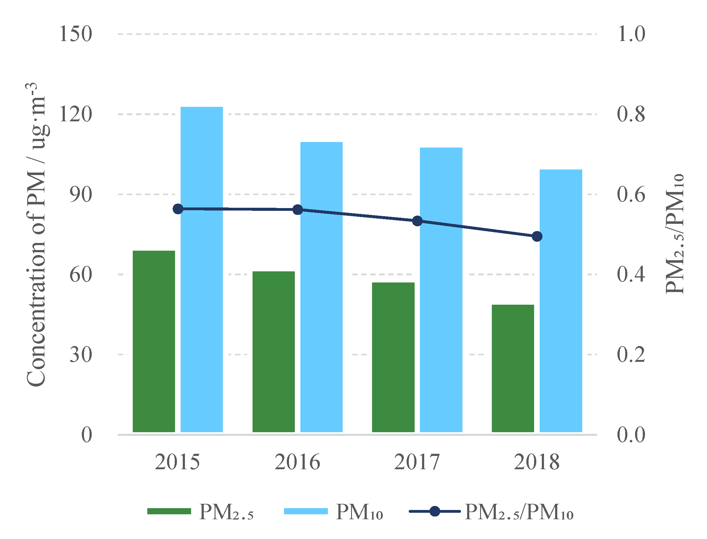
3.2.1. Characteristics at the Annual Scale

The annual average PM2.5 and PM10 concentrations in the study area from 2015 to 2018 were statistically analysed, and the results are shown in Figure 2. Overall, the PM2.5 and PM10 concentrations in the study area decreased each year from 2015 to 2018, with annual average PM2.5 concentrations of 69.9, 62.2, 58.0 and 49.7 μg·m−3, respectively. The annual mean PM10 concentrations were 123.8, 110.6, 108.5 and 100.4 μg·m−3, respectively. The concentration decreased by 23.5 μg·m−3 over four years, with an average annual change of approximately 7.8 μg·m−3. The overall PM2.5/PM10 ratio in the study area reached approximately 0.53, which indicated that PM2.5 was the main component of PM10 in the study area. Moreover, the PM2.5/PM10 ratio decreased each year from 2015 to 2018, with values of 0.56, 0.56, 0.53 and 0.49, respectively, indicating that while the overall PM concentration decreased, and the proportion of PM2.5 to PM10 therefore decreased.
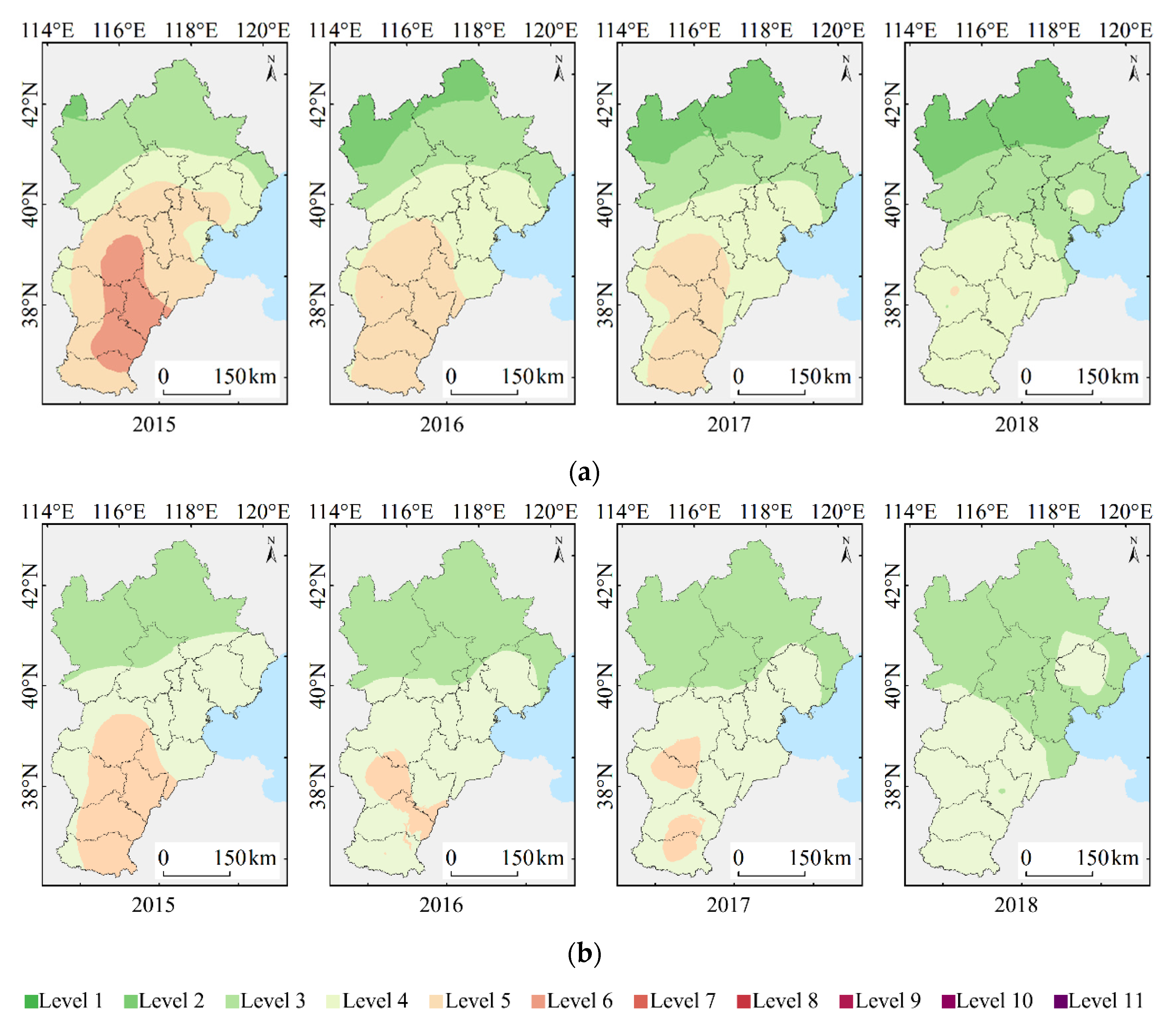
The spatial distribution of the annual mean particle concentration was obtained with the spatial interpolation method, and the results are shown in 
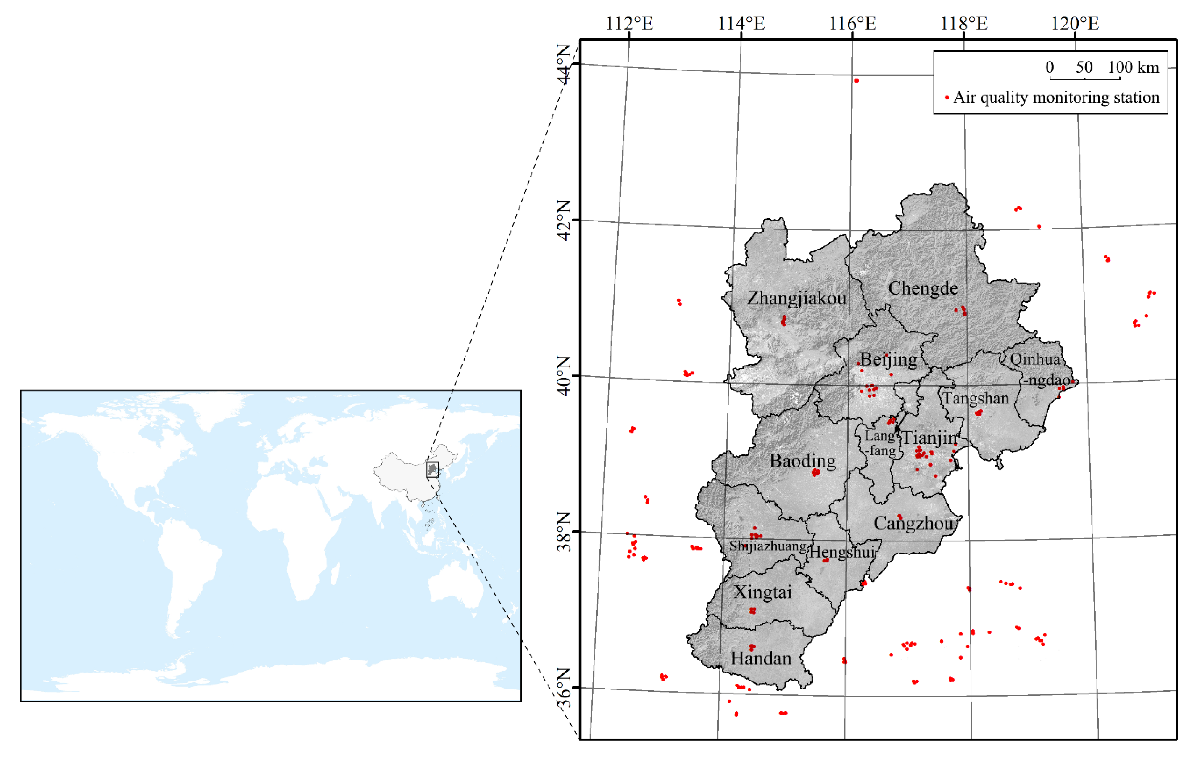
Figure 3. Overall, the trend of PM concentration in the study area was high in the southeast and low in the northwest. The overall concentrations in Chengde, Zhangjiakou and other cities in the north were low, while those in Beijing, Tianjin and other central cities were slightly higher. Relatively high values were mostly concentrated in Xingtai, Hengshui, Handan, Shijiazhuang, Baoding and other cities in the south.
In 2015, the highest annual average PM2.5 concentration reached Level 6 and was mainly distributed in southern cities of the BTH region, accounting for 14.7% of the total area. Nearly half of the experimental region had concentrations exceeding the Level 2 limit, and regions with Level 4, 3 and 2 concentrations accounted for 20.7%, 30.2% and 1.1%, respectively, of the total area. Compared to 2015, the annual average concentration decreased significantly in 2016; the areas with Grade 5 and 6 concentrations in the south shrank rapidly. In addition, areas with annual average concentrations exceeding the Grade 2 limit decreased to 31.9%, while the areas with Grade 4, 3 and 2 concentrations sequentially expanded towards the south, accounting for 30.0%, 26.0% and 12.1%, respectively, of the total area. In 2017, the Level 5 concentration range contracted slightly, with an annual average concentration of 23.5% in the area, exceeding the Level 2 limit, and the areas of Level 4, 3 and 2 concentrations continued to expand southwards, accounting for 32.0%, 26.2% and 18.3%, respectively, of the area. In 2018, the annual average concentration declined considerably, and the areas of Grade 4, 3 and 2 concentrations continued to expand from north to south, with the corresponding areas accounting for 41.8%, 33.6% and 24.4%, respectively, of the total area. However, most of these areas exhibited excellent and good air quality conditions.
In 2015, the highest annual average PM10 concentration reached Level 5, which exceeded the secondary limit of the national standard and was concentrated in the south, accounting for 24.0% of the total area. The lowest level was Level 3, which was largely distributed in the northern part of the study area, accounting for 33.1% of the area. The remaining areas, accounting for 42.9% of the total area, had Level 4 concentrations. In 2016, the Level 5 concentration range contracted, and the Level 2 limit was exceeded in only 6.7% of the whole region. The Level 3 range expanded towards the south, accounting for 43.6% of the total area. The remaining areas, accounting for 49.7% of the total area, all had Level 3 concentrations. In 2017, the areas at each concentration level remained the same as those in 2016, among which the Level 5 concentration range slightly expanded, with Shijiazhuang–Baoding and Handan–Xingtai forming two Level 5 concentration centres, while Level 3 still dominated in the north. In 2018, the concentration declined greatly, Level 5 areas disappeared, and the annual average concentration in the whole region reached below the Level 2 limit. Among the various cities, the southern cities and the northern part of Tangshan, accounting for 44.2% of the total area, mostly had Level 4 concentrations, while the remaining areas reached Level 3 concentrations and accounted for 55.8% of the total area.
It is generally acknowledged that PM2.5 and PM10 are produced by a combination of natural and human activities. Of these components, PM2.5 originates from industrial waste gas, automobile exhaust, fuel combustion and secondary PM formed through a series of reactions, while PM10 originates from natural dust and dust generated by traffic and urban construction [18,19,20,21]. The higher the PM2.5/PM10 ratio is (which may be attributed to automobile exhaust and straw burning), the higher the mass concentration of fine particles in the air, and the more serious the fine particulate pollution and threat to human health. The lower the PM2.5/PM10 ratio is (which may be caused by natural factors such as dust and sandstorms), the higher the mass concentration of inhalable particles in the air [22,23,24,25].
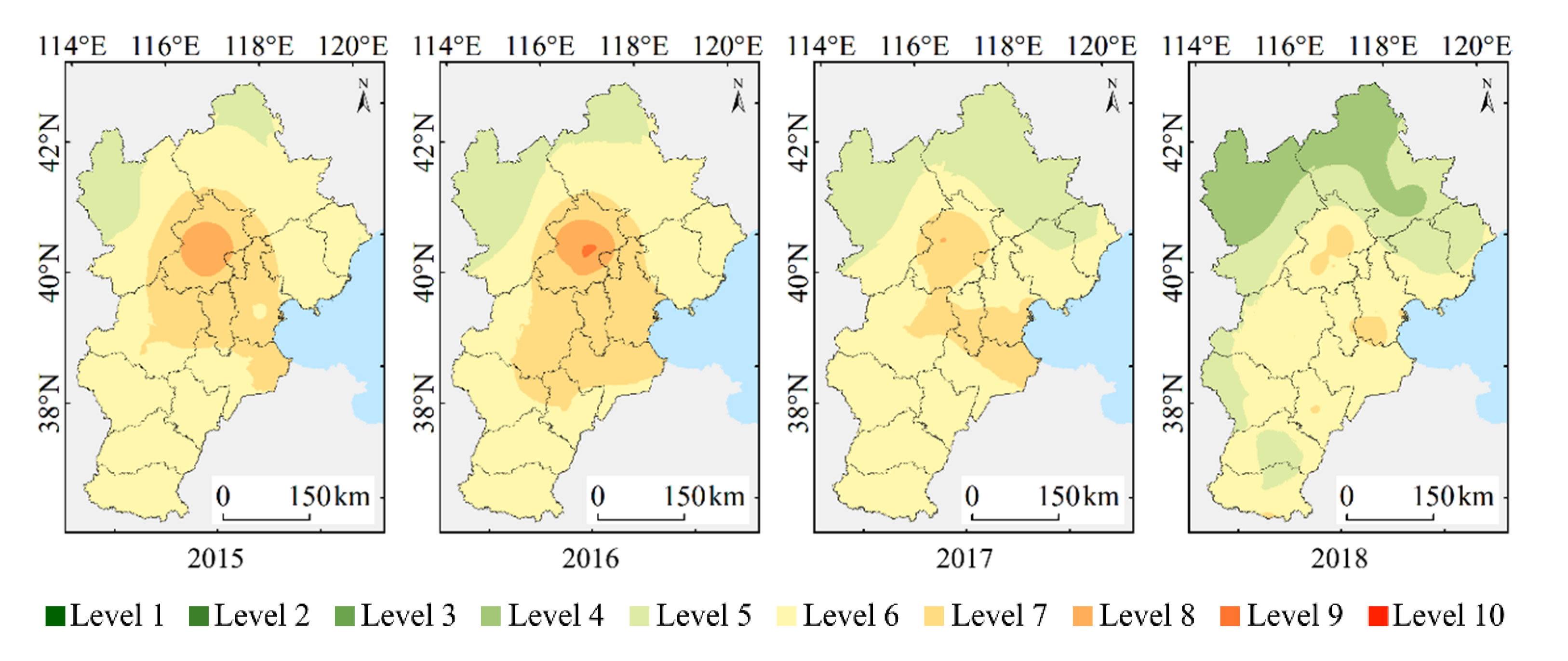
Figure 4 shows the spatial distribution of the annual mean value of the PM2.5/PM10 ratio. The highest value of the PM2.5/PM10 ratio each year was centred in Beijing, followed by Tianjin, Baoding, Langfang and other areas south of Beijing, while the ratio in the mountainous areas and grasslands in the north was lower. The spatial distribution of the ratio displayed a positive relationship with the degree of economic development and intensity of human activities. The road density and traffic volume in Beijing are both large. Motor vehicle exhaust emissions constitute an important source of PM in the atmosphere, which more notably contributes to PM2.5. Human activities in the northern mountains and grasslands are limited, and the proportion of natural emissions of PM sources is high. Especially in seasons with a low vegetation coverage, the proportion of dust, particularly dust particles with larger diameters, in PM sources increases, resulting in a relatively low PM2.5/PM10 ratio. In 2015, the ratio in downtown Beijing reached Level 8, the ratio in Tianjin, Langfang, Baoding and other cities mostly reached Level 7, the ratio in other areas mostly reached Level 6, and the ratio in some northern areas reached Level 5. In 2016, a high value exceeding Level 9 was observed at the centre of Beijing, and the range of areas with Level 8 values expanded south. In 2017, the ratio decreased, and the range of areas with values above Level 7 contracted sharply, while those at Levels 8 and 9 nearly disappeared. In 2018, the ratio further decreased, with only Level 7 values observed in downtown Beijing, Tianjin and Hengshui and Level 3 occurring in the north.
The analysis above indicated that from 2015 to 2018, the PM2.5 and PM10 concentrations and the PM2.5/PM10 ratio all exhibited a declining trend, and the regions with relatively high values contracted or even disappeared, which demonstrated the achievements of emission reduction efforts across the study area. This achievement was closely related to policies and measures such as industrial transformation and upgrading, energy structure reform, strict control of mobile source emissions, and forestland area expansion.

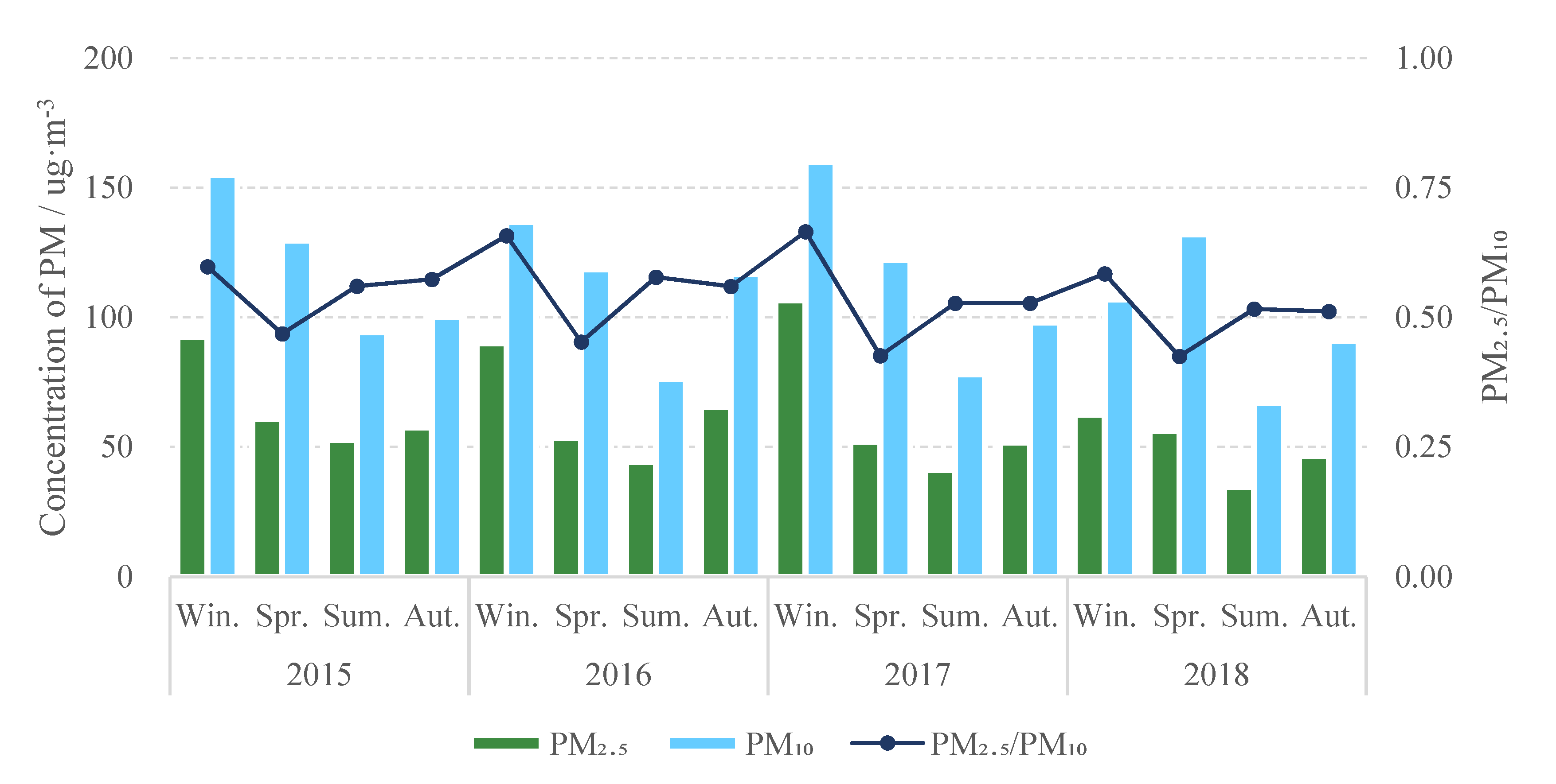
3.2.2. Characteristics at the Seasonal Scale

Statistics of the average seasonal PM2.5 and PM10 concentrations in the study area from 2015 to 2018 were calculated. The results are shown in Figure 5. Overall, there were already stated seasonal differences between the PM2.5 and PM10 concentrations in the study area. The average PM2.5 concentrations in winter, spring, summer and autumn reached 87.8, 55.6, 43.1 and 55.3 μg·m−3, respectively. The average concentrations in winter were approximately twice as high as those in summer, and the average concentrations in spring and autumn were similar to those in winter and summer. The maximum concentration was 106.5 μg·m−3 in the winter of 2017, and the minimum concentration was 34.6 μg·m−3 in the summer of 2018. Hence, the maximum value was approximately 3.1 times the minimum value. The average PM10 concentrations in the four seasons were 139.6, 125.6, 78.9 and 101.5 μg·m−3, respectively. Generally, the concentration in winter was 1.8 times that in summer. The maximum value was 160.0 μg·m−3 in the winter of 2017, and the minimum value reached 67.0 μg·m−3 in the summer of 2018. Thus, the maximum concentration was approximately 2.4 times the minimum concentration. Heating activities in the winter greatly increase the combustion of coal and other energy sources. Moreover, the surface inversion layer often occurs in winter, acting as a lid to block the upward vertical turbulence of air, which prevents the diffusion of particles and retains it in the atmosphere for a longer time [26,27]. In addition, due to the withering of vegetation, the particle adsorption and blocking ability of the vegetation is greatly reduced, and the particle concentration is therefore highest in the winter [13]. In summer, the temperature rises, air convection is strong, and the horizontal and vertical transport capacities of the atmosphere are notable, which enhances its particle dilution and diffusion capacities. Furthermore, the lush vegetation during the growing period strongly affects particle sedimentation. In addition, increases in precipitation play a notable role in scouring and inhibiting particles, thus the particle concentration in summer is generally low [28,29]. Meteorological conditions such as temperature, humidity, precipitation and wind speed, and natural conditions such as vegetation cover in spring and autumn vary from those in winter and summer. In addition, frequent dust weather conditions and large-scale straw burning are the main sources of PM in spring and autumn, respectively. The PM2.5/PM10 ratio also exhibits an obvious seasonal regularity, with the average values in the four seasons reaching 0.63, 0.44, 0.55 and 0.54, respectively. The PM2.5/PM10 ratio is the highest in winter, lowest in spring and moderate in summer and autumn. This is mainly attributable to the dry air and scarce precipitation in spring, which results in a dry and unconsolidated surface. Furthermore, the vegetation coverage is relatively low, and the high average wind speed is attributed to stronger winds. These conditions jointly promote the easy entry of surface dust into the atmosphere [12,23,30]. However, PM10 have a larger diameter, and the contribution rate of dust to PM10 is higher than that to PM2.5, which is one of the reasons for the relatively low PM2.5/PM10 ratio in spring [31]. In winter, the temperature is low, people in the study area start to use heating sources more, and coal-based energy consumption increases [32,33,34]. Moreover, incomplete motor vehicle fuel combustion occurs due to the low temperature and air pressure, all of which contribute to higher PM2.5 levels, resulting in an increased PM2.5/PM10 ratio in winter [12,34].
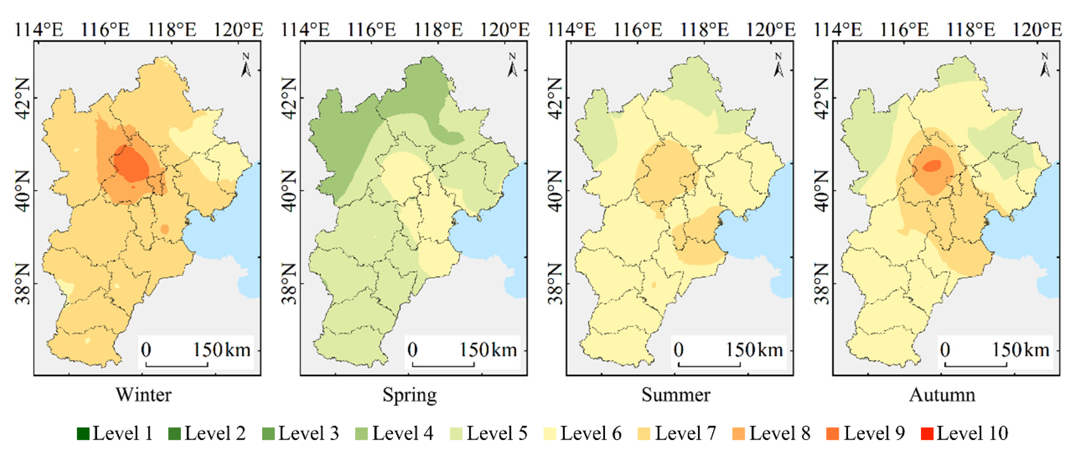
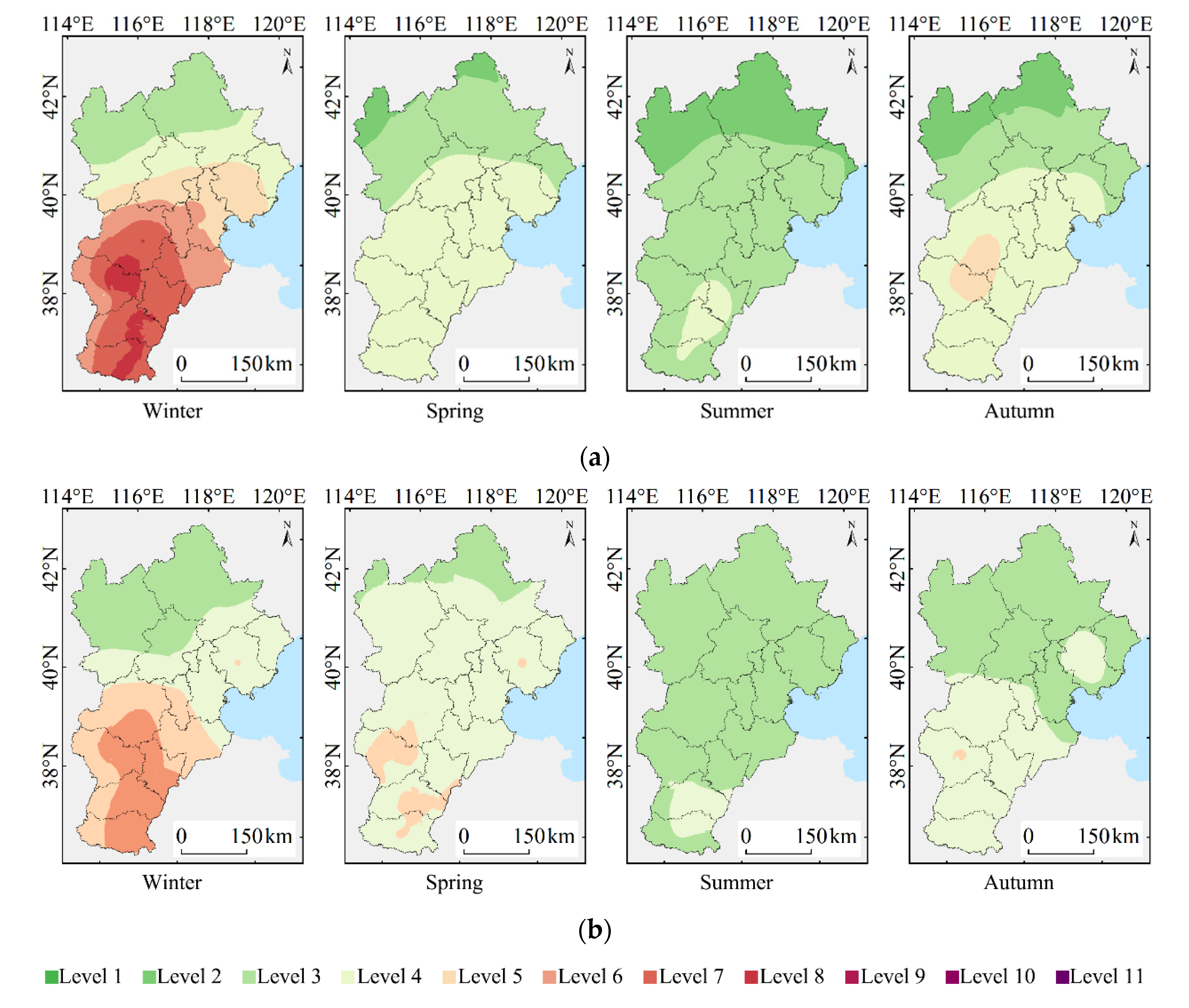
The spatial distribution of the seasonal mean PM concentration was determined with the spatial interpolation method, and the results are shown in Figure 6. In winter, the average seasonal PM2.5 concentration was the highest among the four seasons, with the highest value reaching Level 8, which is moderate pollution. Shijiazhuang–Baoding and Xingtai–Handan formed two centres, accounting for 5.5% of the total area. The concentration gradually decreased from these high-value centres to the surrounding areas, of which the southern areas mostly had concentrations of Level 5 and above, and areas with Level 5, 6 and 7 ratios reached 16.2%, 16.6% and 21.0%, respectively. In addition, 59.3% of the area experienced light or moderate pollution. Most of the concentrations in the north reached Levels 3 and 4, accounting for 22.6% and 18.1%, respectively, of the total area. The concentration in spring was notably lower than that in winter, and the whole area did not meet the pollution standard. In the south, Level 4 concentrations were observed, accounting for 61.4% of the total area. Most of the concentrations in the north reached Levels 2 and 3, accounting for 5.6% and 33.1%, respectively, of the total area. In summer, the concentration was the lowest of the year, and in the south, the concentrations mostly reached Levels 3 and 4, with areas of 67.2% and 6.1%, respectively. The range of areas with Level 2 concentrations expanded southward, accounting for 26.7% of the total area, and their air quality was excellent. The concentration in autumn slightly increased, approaching the average regional concentration in spring, but there were differences in its spatial distribution: the concentration in the south was slightly higher than that in spring, and the concentration in the north was slightly lower than that in spring. Moreover, Level 5 concentrations were observed in the south, accounting for 5.7% of the area, and the areas with Level 2, 3 and 4 concentrations reached 15.6%, 28.6% and 50.1%, respectively.
The average seasonal PM10 concentration was also highest in winter, and the ranges of areas with Level 5 and 6 concentrations, accounting for 21.0% and 17.4%, respectively, of the regional area, were concentrated in the southern region, which was mildly polluted. Areas with Level 3 and 4 concentrations occupied most of the north, accounting for 32.1% and 29.4%, respectively, of the regional area. In the spring, the relatively high-value area in the south contracted, and the change in the PM10 concentration distribution in the north exhibited a different trend from that of the PM2.5 concentration distribution. The concentration increased slightly, but the relatively low-value area contracted northwards, which was related to the frequent dusty weather conditions in spring. Level 5 concentrations were observed in southern cities, accounting for 7.8% of the total area. The range of areas with Level 4 concentrations was reduced to 10.8%, while the rest of the area exhibited Level 3 concentrations, accounting for 81.4% of the regional area. In summer, the concentration was the lowest and the concentration in the whole region remained below Level 4. Except for areas with Level 4 concentrations, which accounted for 6.4% of southern cities such as Xingtai and Handan, the remaining area (93.6%) exhibited Level 3 conditions. In autumn, the concentration rose slightly. Except for the Level 5 concentrations in Shijiazhuang, which accounted for 0.3% of the area, all other areas failed to meet the pollution standard, with the ranges of areas with Level 3 and 4 concentrations accounting for 55.4% and 44.4%, respectively, of the total area.
Figure 7 shows the spatial distribution of the seasonal mean value of the PM2.5/PM10 ratio. The PM2.5/PM10 ratio varied greatly between different seasons. In winter, the ratio was the highest, with a Level 9 value observed at the centre of Beijing, Level 8 values occurring in the surrounding areas and Level 7 values distributed in the other areas. PM2.5 was the main component of PM10. The spring ratio was the lowest of the whole year, with Level 6 values observed in Beijing, Tianjin, Langfang and Cangzhou, Level 4 values only occurring in certain areas of Zhangjiakou and Chengde in the north, and Level 5 values distributed in the other areas. In summer, two Level 7 centres were formed in Beijing and Tianjin, whereas most of the other regions reached Level 6. In autumn, the ratio in Beijing increased, exhibiting Level 8 and 9 values, while the range of areas with Level 7 values slightly expanded, and other areas exhibited similar levels to those in summer.
The analysis above indicated that the PM2.5 and PM10 concentrations and PM2.5/PM10 ratio in the study area exhibited significant seasonal regularity. In the different seasons, meteorological conditions such as temperature, humidity, precipitation, wind speed and air pressure were quite different and imposed varying influences on the processes of particle generation, emission, diffusion and transmission. Moreover, vegetation growth exhibited obvious seasonal regularity, and PM inhibition or promotion differed between the various seasons. The types and intensities of human activities were also closely related to season, especially in the study area in North China, where heating in winter requires a large amount of energy from sources such as coal, which notably impacts the PM concentration and is one of the main reasons for the frequent occurrence of winter smog in the study area in recent years.

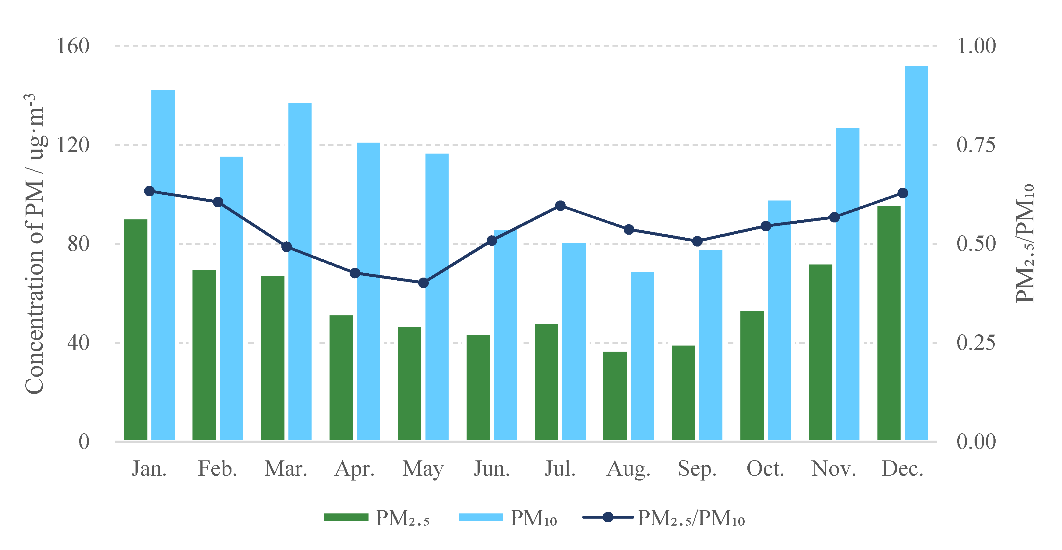
3.2.3. Characteristics at the Monthly Scale

Statistics of the monthly mean values of the PM2.5 and PM10 concentrations in the study area from 2015 to 2018 were computed. The results are shown in Figure 8. In general, the PM2.5 and PM10 concentrations in the study area exhibited obvious periodicity with the annual cycle. Generally, peak and valley values occurred each year. Every year, the peak PM2.5 concentration mostly occurred in December and January, when the average monthly concentration reached 96.1 and 90.7 μg·m−3, respectively. The valley value mostly occurred in August and September, when the average monthly concentration reached 37.2 and 39.7 μg·m−3, respectively. The highest value was 135.7 μg·m−3 in December 2015, and the lowest value was 27.9 μg·m−3 in September 2018. Hence, the highest value was 4.9 times the lowest value. The monthly mean PM2.5 concentration demonstrated a decreasing trend from January to June. After a slight increase in July, the concentration reached its lowest value in August and then increased from August to December. The main reason for the slight increase in concentration in July could be that higher temperatures and increased precipitation promote the occurrence of photochemical reactions and, thus, facilitate the formation of secondary particles. Each year, the peak PM10 concentration mostly occurred in December, January and March, and the average monthly concentration reached 152.9, 143.1 and 137.6 μg·m−3, respectively. The valley values mostly occurred in August and September, and the average monthly concentrations reached 69.3 and 78.4 μg·m−3, respectively. The highest value was 199.3 μg·m−3 in December 2015, and the lowest value was 57.6 μg·m−3 in August 2018. Hence, the highest concentration was 3.5 times the lowest concentration. After the average monthly PM10 concentration decreased from January to February, it rose slightly in March and exhibited a gradual downwards trend from March to August. After reaching the lowest value in August, the concentration increased from August to December. The main reason that the concentration in March was slightly higher than that in February could include the melting of snow and ice due to the rising temperature in spring, and since most vegetation had not yet entered the growing season, this led to surface dust exposure to air, which easily generated dusty weather under windy conditions and promoted the entry of larger-sized particles into the atmosphere. The PM2.5/PM10 ratio also revealed a periodic trend, which usually formed double peaks and double valleys in a given year: the PM2.5 and PM10 levels were high in December or January of the following year, and the first peak value was formed due to the increase in PM2.5 concentration facilitated by coal combustion and the ground inversion layer phenomenon. Frequent dusty weather in spring gradually enhanced the ratio, and the first valley value was reached in May. Subsequently, the rapid increase in temperature and humidity promoted the chemical transformation of secondary organic aerosols and accelerated the PM2.5 formation process. In addition, because the scouring effect of precipitation on PM10 was greater than that on PM2.5, the ratio reached its second peak value in July. A decrease in precipitation, temperature, humidity and wind speed caused a slight reduction in the ratio after July and formed the second valley in September. Subsequently, with the rapid drop in temperature and arrival of the heating period, the amount of burning of coal and other energy sources rapidly increased, a large amount of PM2.5 was discharged into the air, and the ratio reached a peak value again.
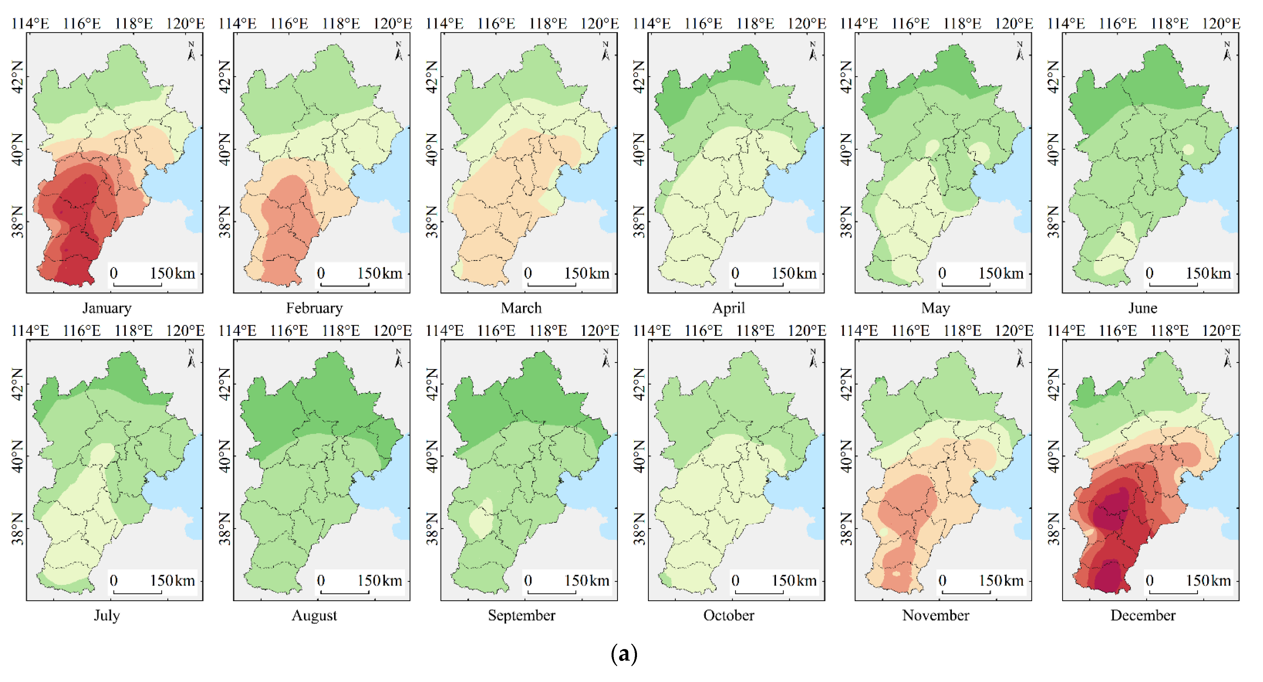
The spatial distribution of the monthly mean particle concentration was calculated with the spatial interpolation method, and the results are shown in Figure 9. The monthly mean PM2.5 concentration exhibited a large spatial difference, where the concentration in the northern region was low and constant, and most of the concentrations reached Levels 2, 3 and 4 throughout the year. There was a large fluctuation in the south, with Level 9 concentrations were observed in December when the concentration was the highest and Level 3 concentrations observed in August when the concentration was the lowest. In January, 58.6% of the whole area was slightly or moderately polluted, and high values were concentrated in the south, of which areas with Level 7 and 8 concentrations accounted for 15.5% and 16.0%, respectively, of the total area. From February to April, the high-concentration range contracted rapidly, areas with Level 7 and 8 concentrations disappeared in February, those with Level 6 concentrations disappeared in March, those with Level 5 and above concentrations all disappeared after April, and the concentration across the whole region declined to match the national secondary standard. From May to August, the concentration dropped further, and by August, areas with Level 4 concentrations completely disappeared and the range of areas with excellent air quality reached 41.8%, the highest of the whole year. From September to November, the concentration began to rise rapidly, and in September, Level 4 concentrations reappeared. In November, Level 5 and 6 concentrations reoccurred in the southern region, covering 53.5% of the total area. In December, the concentration was the highest of the whole year. The Shijiazhuang–Baoding and Xingtai–Handan areas contained two heavily polluted areas with concentrations reaching Level 9, accounting for 8.1% of the total area. Areas with concentrations at Levels 7 and 8 accounted for 27.7% of the total area, and those with concentrations at Levels 5 and 6 accounted for 26.4% of the total area. Of the whole region, 62.1% of the area was lightly, moderately or heavily polluted, which was the highest pollution level of the whole year.
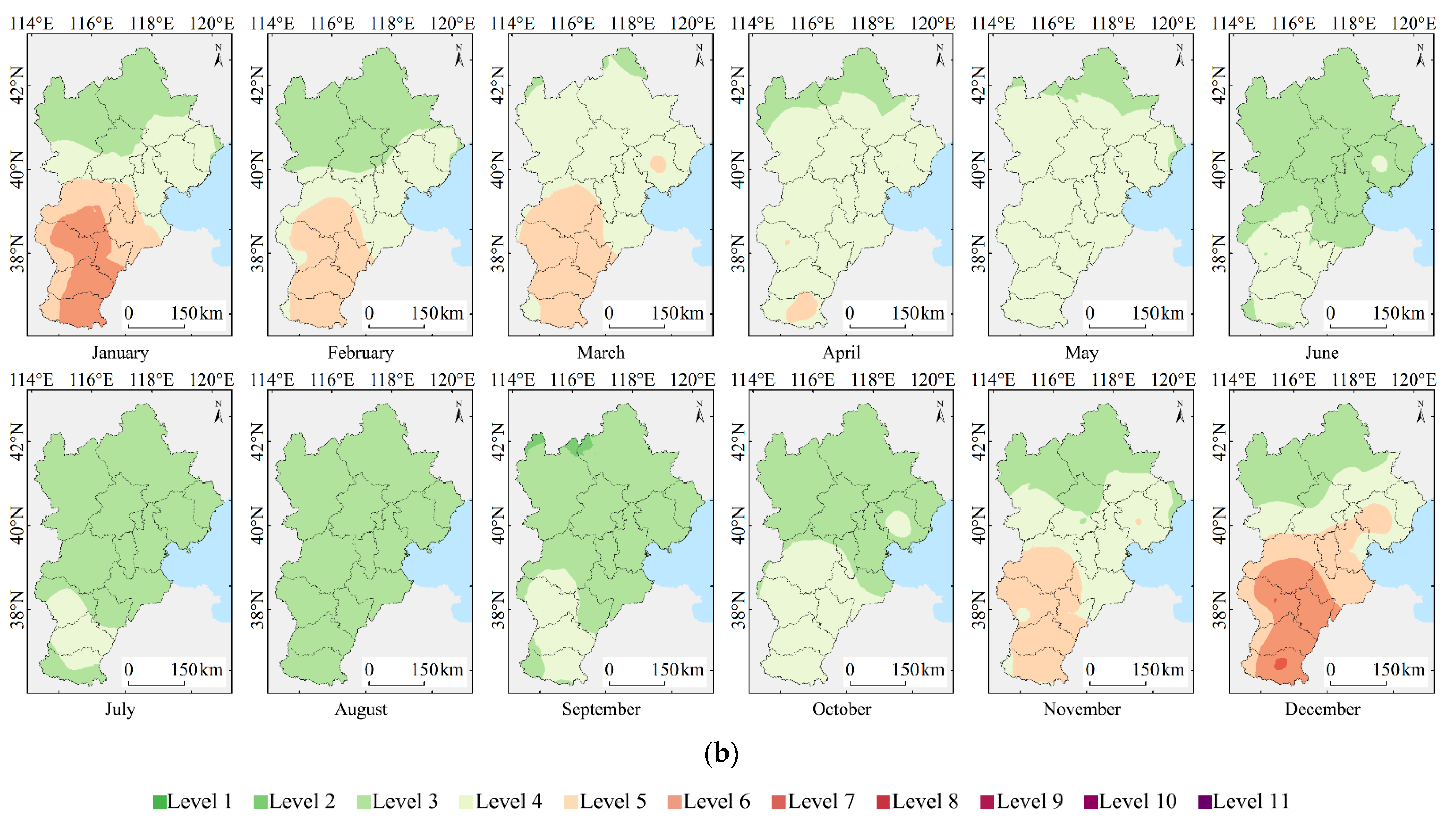
Compared to PM2.5, the spatial difference and temporal fluctuation in the monthly mean PM10 concentration were relatively limited. In January, the ranges of areas with Level 3–6 concentrations gradually transitioned from north to south, and 38.9% of the southern area exhibited light pollution levels. In February, the concentration decreased, and Level 6 concentrations disappeared. In March, the monthly concentration increased, especially in the northern region, with the Level 4 concentration range expanding greatly from south to north, while a Level 5 concentration was observed in Tangshan. From April to August, the concentration dropped rapidly. In May, Level 5 concentrations disappeared, and the concentration across the whole region declined below the national Level 2 standard. In August, Level 4 concentrations disappeared, and the whole region had Level 3 concentrations. In September, Level 4 concentrations were observed again and remained through the rest of the year. From October to December, the concentration increased rapidly. In November, Level 5 concentrations reoccurred, and in December, Level 6 concentrations were observed again. In Shijiazhuang and Handan, even Level 7 concentrations were reached. The moderately polluted area accounted for 0.5% of the total area, and 48.1% of the whole area was slightly or moderately polluted.
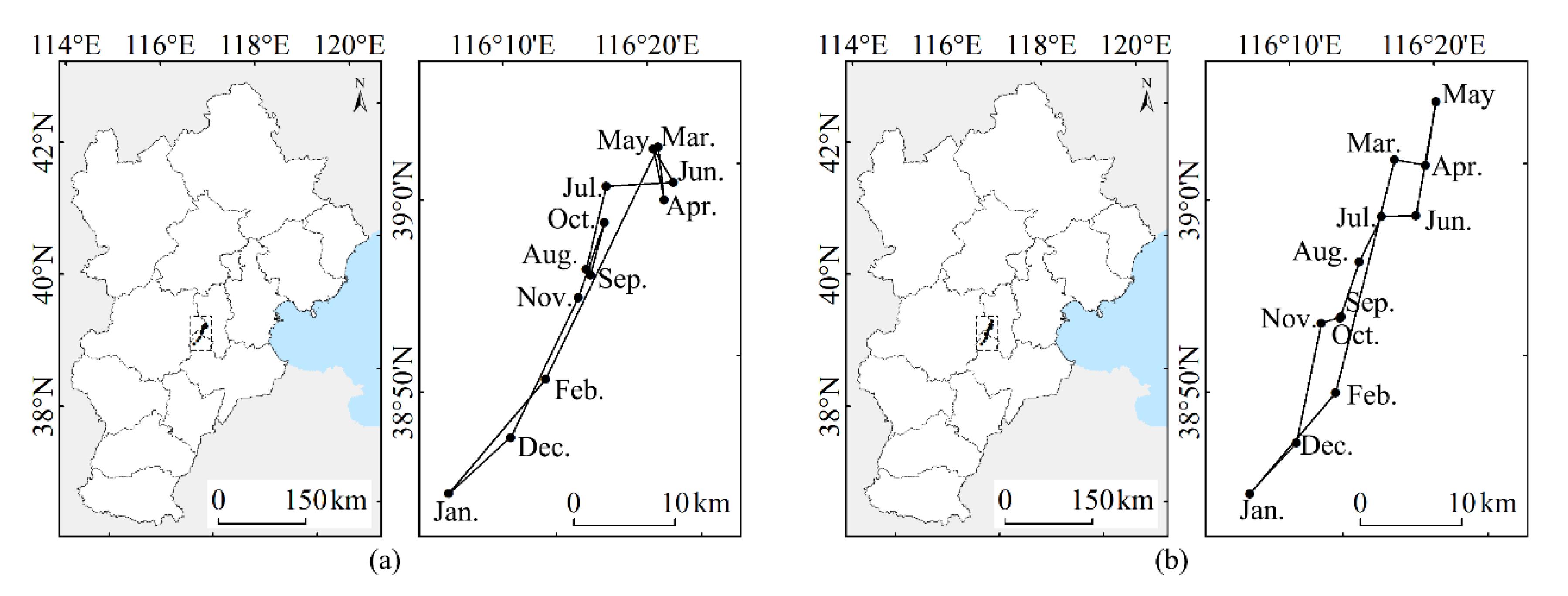
The spatial centre of gravity was calculated for the average monthly PM2.5 and PM10 concentrations each month, and the migration trajectory of the centre of gravity in each month was determined. The results are shown in Figure 10. The results indicated that the average monthly centre of gravity of the PM2.5 and PM10 concentrations in the BTH region was concentrated along the borders of Langfang, Cangzhou and Baoding, and the migration trajectory exhibited a certain regularity. Generally, the migration trend of the centre of gravity throughout the year demonstrated that the centre moved rapidly from southwest to northeast and then gradually moved back to the southwest from the northeast. In January, the centre of gravity was located in the southwest. From February to March, the centre of gravity moved sharply to the northeast, remained in the northeast from March to June, moved slightly towards the west in July, remained west of Central China from August to November, moved sharply towards the southwest in December, and returned to the southwest in January of the following year. In winter (December, January, and February), the centre of gravity was located in the southwest, which indicated that although the overall concentration in the area in winter increased, the southwestern part of the study area had a concentrated, high pollution level. In spring (March, April, and May), the centre of gravity was located in the northeast, which indicated that there was a greater decrease in concentration in high-value areas in the south from winter to spring than in the north, which may be related to the frequent occurrence of dusty weather conditions in the north. In summer (June, July, and August) and autumn (September, October and November), the centre of gravity remained at the centre of the region, which indicated that the degree of concentration change at each location across the region remained relatively stable and that the overall change was similar.

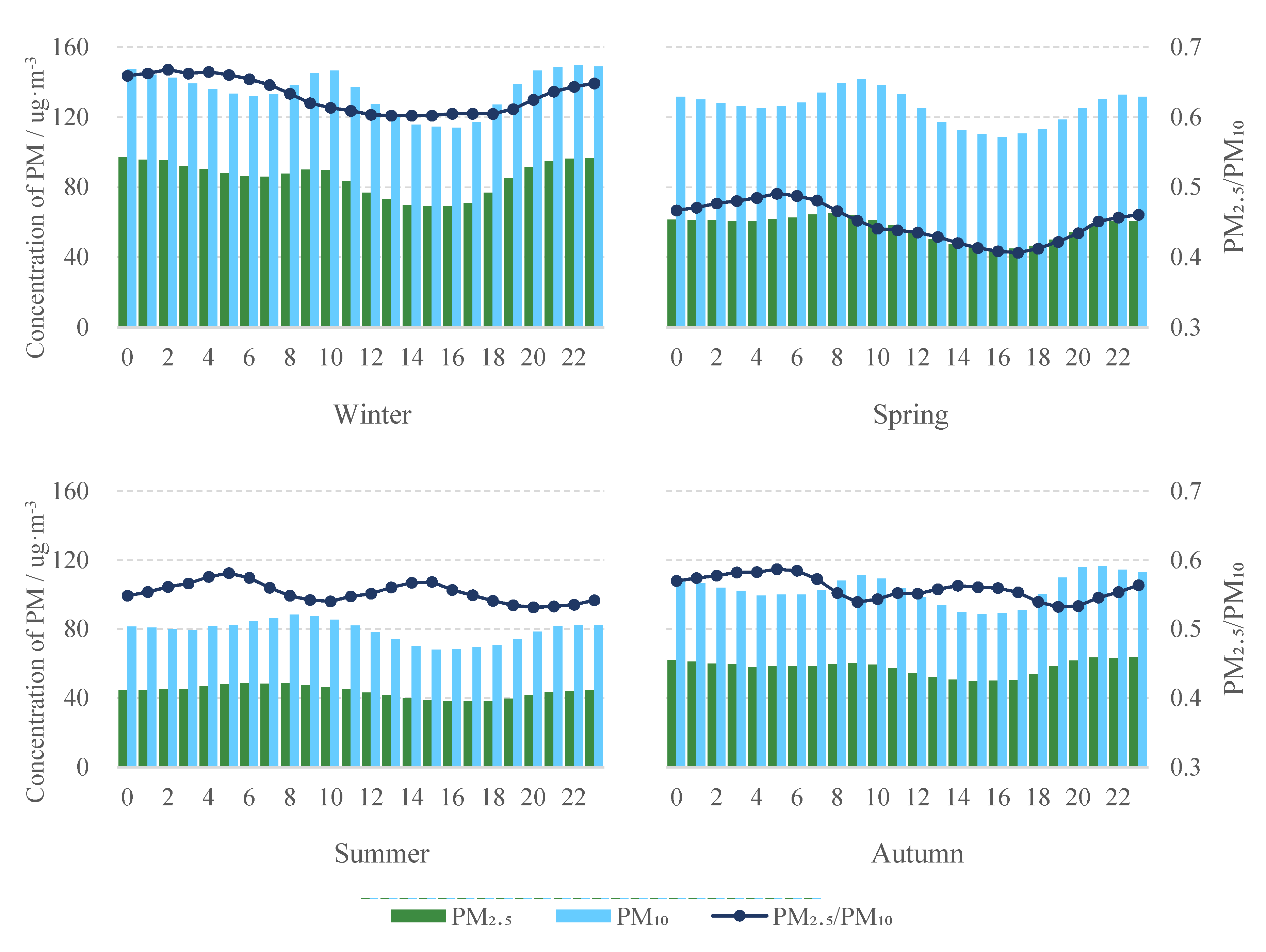
3.2.4. Characteristics at the Hourly Scale

Hourly mean values of the PM2.5 and PM10 concentrations in the study area from 2015 to 2018 were calculated for each season, and the results are shown in Figure 11. The average PM concentration scale indicated a diurnal cycle, mostly revealing a trend of double peaks and double valleys. At night, the temperature was relatively low, the boundary layer height decreased, and the atmospheric turbulence activity weakened, which did not facilitate PM diffusion. Hence, the PM concentration was higher at night or in the early morning, and the first peak was reached. Human activities greatly decreased at night, as most of the population was sleeping, and the PM concentration gradually dropped at night, reaching the first valley in the early morning. With the sun rising in the morning, the temperature gradually increased, human activities increased, and the speed of secondary particle generation increased. Moreover, during the morning rush hour period, motor vehicles discharged a large amount of tail gas into the atmosphere and dislodged road dust, and the particle concentration reached its second peak in the morning [27]. Subsequently, with the increasing boundary layer height, the atmospheric turbulence activity was enhanced, and these conditions facilitated PM diffusion. Furthermore, after the morning peak, the traffic volume on the roads decreased slightly, so the PM concentration was reduced to a certain extent and declined further until it reached the second valley in the afternoon. In the evening, as the sun went down, the temperature rapidly dropped, and with the traffic peak at night and the sharp increase in kitchen oil smoke emissions at dinner time, PM continuously accumulated in the atmosphere and the concentration rose again and reached a peak value in the evening or early morning [28,29,35].
The timing of peak and valley PM concentrations during the four seasons and their corresponding concentrations are listed in Table 3. The peak value at night mostly occurred from 22:00 to 0:00 the next day, the valley during the morning mostly occurred from 4:00 to 7:00, the peak value in the morning mostly occurred from 8:00 to 10:00, and the valley in the afternoon mostly occurred from 15:00 to 17:00. Usually, the morning peak occurred between ~7:00 and 9:00 and the evening peak occurred between 17:00 and 19:00. The morning and evening peaks imposed a certain delayed effect on the PM concentration variation [13,36,37,38]. Comparing the two peaks and valleys during the same season, the results indicated that during each season, the valley in the afternoon was obviously lower than that in the morning, which was the lowest value throughout the whole day. This finding verified that the favourable meteorological conditions for PM diffusion in the afternoon obviously affected the PM concentration reduction. There were seasonal differences between the heights of the two peaks. The night peak in autumn and winter was higher than the morning peak, but the opposite was true in spring and summer. The atmosphere in autumn and winter was more stable than that in summer, and relatively calm weather occurred, which resulted in PM sedimentation and diffusion taking more time than in summer. Moreover, the temperature in winter was low and the night lasted longer. The heating demand at night greatly increased the amount of burning of coal and other energy sources, resulting in the highest concentration at night. Comparing the occurrence times of the peaks and valleys among the four seasons, we observed that the peaks in the morning occurred the earliest in summer and the latest in winter, while the occurrence times of the valleys in the afternoons were the opposite, which was directly related to sunrise, sunset and sunshine duration. The morning temperature rise occurred later than in summer, and the afternoon temperature drop occurred earlier. In addition, the PM2.5 concentration at night in summer remained relatively stable, increasing slowly from 17:00 to 8:00 the next day, with no obvious night peak or early morning valley. A single peak and a single valley were observed throughout the whole day, which may be related to factors such as higher summer temperatures, longer sunshine durations, shorter night periods, and more persistent human activities. In addition, in summer, construction and earth excavation activities occurred in more cities at night, and popular evening dining activities could also promote higher concentrations on summer nights [39].
The PM2.5/PM10 ratio exhibited a single peak and a single valley in winter and spring, and the ratio slowly decreased during the day after reaching the full-day peak in the morning. The PM2.5/PM10 ratio then gradually increased after reaching a valley in the evening. In summer and autumn, a pattern with double peaks and double valleys was observed, which differed from that in winter and spring in that the ratio increased from approximately 9:00 to 15:00, which may be attributed to the relatively high temperature and humidity during the day in summer and autumn, thus intensifying the occurrence of secondary reactions and increasing the PM2.5 concentration. The surface temperature is generally low at night, and inversion occurs when the surface temperature is lower than the air temperature. Consequently, stable atmospheric conditions limit vertical airflow, which is conducive to the dry settlement of coarse particles and accumulation of fine particles, resulting in a gradual increase in the night-time ratio. With increasing human activity intensity during the day, rough road dust becomes resuspended in the air. In addition, a large amount of construction dust greatly influences the PM10 concentration, which gradually reduces the PM2.5/PM10 ratio. In summer and autumn, the afternoon valley occurred slightly later than in winter and spring, which was caused by the slightly later inversion occurrence time in summer and autumn than in winter and spring [30,40,41].

3.3. Variation Patterns of the Atmospheric Particulate Matter Concentration

The optimized function models in Section 2.4 were employed to fit the monthly mean values of the PM2.5 and PM10 concentrations in the whole study area and in individual cities. The results are shown in Figure S1. The fitting parameters in the whole study area and each city were statistically analysed, and the results are listed in Table S1.
According to the goodness-of-fit R2 value, the fitting R2 values of PM2.5 and PM10 in the study area were 0.74 and 0.58, respectively, which verified that the improved model could better reflect the variation pattern of the monthly mean concentration. Comparing the fitting results for the different cities, the fitting effect was obviously better in areas with higher overall PM concentrations than in areas with lower concentrations, which was attributed to the larger difference between the peak and valley values in areas with higher concentrations, thereby revealing a more obvious periodic fluctuation trend. However, in areas with low concentrations, the concentration difference in each month was small, so the influence of random factors on the concentration was obviously greater than that in areas with high concentrations that exhibit high randomness, which slightly reduced the fitting effect. For example, the monthly mean value of the PM2.5 concentration in Zhangjiakou fluctuated slightly at a low grade, with a monthly mean value of only 32.26 μg·m−3 and the highest value of only 55.42 μg·m−3. The influence of season on concentration fluctuation was not obvious, resulting in a low fitting accuracy. Errors occurred in the expressions of Dt, Ft and other parameters in the fitting equation, which could not be compared with the fitting parameters between different regions.
The fitting R2 value of PM2.5 in most cities was higher than that of PM10, which demonstrated that PM2.5 exhibited a more notable periodic variation pattern than that of PM10. This may be attributed to the close relationship between PM2.5 and human activities, and the obvious difference in concentration between the four seasons was caused by various human factors, such as coal burning for heating in winter and increased motor vehicle emissions. In contrast, PM10 is typically more susceptible to natural conditions, with irregular fluctuations to a certain extent and a relatively low periodicity, which resulted in a slightly lower fitting accuracy than that for PM2.5 Among the cities, only Zhangjiakou and Qinhuangdao attained a higher fitting R2 value of PM10 than that of PM2.5, which may have occurred because the intensity of human activities in these two cities was lower than in the other cities and the relationship between PM sources and natural emissions was closer, especially in the spring, when frequent dusty weather greatly influenced the PM level. Hence, the change in the PM10 concentration exhibited a greater regularity than that in the PM2.5 concentration.
From an average concentration perspective, the average PM2.5 and PM10 values in the study area were 59.93 and 110.82 μg·m−3, respectively, which were still higher than the standard limits of 35 and 70 μg·m−3, respectively, stipulated in the Environmental Air Quality Standard. The order of PM2.5 and PM10 concentrations in the various cities were basically consistent. The PM10 concentration was generally higher in areas with higher PM2.5 concentrations, and the areas with higher average concentrations were mostly concentrated in the south of the study area. The relatively well-developed industries in the southern cities provided more sources of PM emissions, and the topographical features of the Taihang Mountains in the west did not promote PM diffusion, resulting in relatively high concentrations. The population density in the northern cities is low, and the proportion of anthropogenic emissions relative to other PM sources is small. In addition, forests and grasslands can inhibit ground PM suspension, which facilitates dry deposition of PM from the air, and results in a relatively low PM concentration.
The PM2.5 and PM10 concentrations in the study area exhibited an accelerated downwards trend overall. Among the cities, the PM2.5 concentration in all parts of the study area revealed downward trends to varying degrees, among which the concentration in all cities declined from 2017 to 2018 and the rate of decline accelerated. The PM10 concentration remained stable at a low grade in the northern cities, while that in the other cities rapidly decreased. The fitting results once again verified that PM pollution in the study area was greatly mitigated from 2015 to 2018.
Considering the amplitude Dt, the amplitude of PM2.5 in most cities was larger than that of PM10, which demonstrated that the relative fluctuation in PM2.5 was slightly stronger than that in PM10. In addition, the amplitude exhibited an obvious north–south pattern. Southern cities such as Cangzhou, Hengshui, Baoding, Shijiazhuang, Xingtai and Handan attained larger amplitudes, while northern cities such as Beijing, Tianjin, Tangshan, Qinhuangdao and Chengde attained smaller amplitudes, which indicated that the fluctuation amplitude in the southern region was generally larger than that in the northern region.
Considering the deformation factor Ft, the fitted Ft value of PM2.5 in most cities was larger than that of PM10, which indicated that the PM10 concentration in these cities increased and decreased more gently than did the PM2.5 concentration during a given period. In regard to PM2.5, the Ft value in most cities was greater than 1, which indicated that these cities exhibited longer durations of low values and shorter durations of high values. Moreover, the Ft value in the southern cities was generally greater than that in the northern cities, which indicated that the difference between the durations of high and low values in the southern cities was larger than that in the northern cities. Regarding PM10, the Ft values in Beijing, Tangshan, Qinhuangdao, Chengde and other northern cities were all less than 1, which indicated that the duration of high values in these cities was longer than that of low values, which occurred due to the frequent dusty weather conditions in spring extending the duration of high PM10 values. However, the Ft values in Handan, Hengshui, Xingtai, Baoding, Shijiazhuang and other southern cities were all greater than 1, indicating that low values lasted longer than high values.
From the point of view of the Gt phase, the Gt value in each city ranged from 0 to ~2.5, indicating that the peak value occurred in winter or spring. Comparing the Gt values between the different regions, the Gt values of PM2.5 in the different cities were similar, but the Gt values of PM10 were relatively different. The Gt values in the northern cities, such as Zhangjiakou, Chengde and Qinhuangdao, were significantly higher than those in the other cities, which was affected by the frequent dusty weather conditions in spring. Comparing the Gt values of the fitting results for PM2.5 and PM10 between the different cities, little differences occurred between these values among all cities, and the Gt values of PM2.5 were all larger than those of PM10, which indicated that the PM2.5 peak in all the cities occurred slightly earlier than that of PM10, which occurred because both the PM2.5 and PM10 levels were higher in winter, but the decline in PM2.5 was obviously larger than that in PM10 in spring. Consequently, the PM10 concentration was relatively high in spring, which caused the average peak value to occur slightly later than that of PM2.5, which differed from that of PM2.5.
Considering the offset factor Ht, the Ht values of the fitting results for PM2.5 in each city were all positive, which indicated that the PM2.5 valley in each city occurred far from the last peak and closer to the next peak, i.e., the concentration decreased slowly and increased rapidly. Among the Ht values of the PM10 fitting results in each city, the values in Zhangjiakou, Chengde and Qinhuangdao were all negative, which indicated that their valleys occurred closer to the last peak and farther from the next peak. In particular, the concentration decreased rapidly and increased slowly, while the trend in the other cities was the opposite.

4. Conclusions

In this manuscript, based on air pollutant concentration data from ground air quality monitoring stations, we analysed the spatio-temporal distribution changes in atmospheric PM concentration across the BTH region in China from 2015 to 2018 at yearly, seasonal, monthly and hourly scales. Then, based on an optimized model, the periodic variation in the atmospheric particle concentration was fitted, and the variation trend of the atmospheric particle concentration was analysed considering the key coefficients of the fitting results. Overall, from 2015 to 2018, the annual average PM2.5 and PM10 concentrations in the study area decreased each year, and the number of days with excellent and good air quality grades increased. Moreover, the PM2.5/PM10 ratio decreased every year, which demonstrated that the series of air pollution prevention and control measures implemented in the BTH region in recent years were quite effective and the PM pollution situation has greatly improved. In most cities, the PM concentration generally revealed a downwards trend. In each cycle, the duration of high values was shorter than that of low values, and the concentration decline rate was lower than the increase rate. There were significant differences in the concentration variation patterns between northern and southern cities. The concentration in southern cities was higher and the fluctuation range was larger. The difference between the durations of high and low values was larger than that in the northern cities, and the peak and valley values occurred slightly earlier. Other conclusions were as follows:
(1) At a monthly or seasonal scale, the PM2.5 and PM10 concentrations exhibited a significant periodic pattern, which was characterized by highest values in winter and lowest values in summer. The highest average monthly concentrations were mostly observed in December and January, and the lowest values mostly occurred in August and September. The PM2.5/PM10 ratio was generally highest in winter and lowest in spring. Climate, vegetation cover, coal combustion, etc. constituted the main reasons for concentration differences between the various seasons.
(2) The hourly mean PM2.5 and PM10 concentrations throughout the day mostly indicated a pattern of double peaks and double valleys, in which peak values were reached at night and in the morning, and valleys occurred in the morning and afternoon. The PM2.5/PM10 ratio exhibited a single peak and a single valley in winter and spring and double peaks and double valleys in summer and autumn. The diurnal fluctuation trend was closely related to weather conditions and human activities.
(3) Spatially, the PM2.5 and PM10 concentrations were mostly high in the southeast and low in the northwest. High values were largely concentrated in the southern cities of the BTH region, while values in the northern cities were relatively low. The PM2.5/PM10 ratio was highest in Beijing and decreased in the surrounding areas. The distribution of low and high values was related to the difference in formation conditions between PM2.5 and PM10.
(4) The traditional function model was improved, and the average R2 value of the monthly mean fitted PM2.5 and PM10 concentrations in each city was enhanced from 0.49 to 0.65. Compared to the traditional model, the fitting accuracy and effect were greatly improved and useful information on the change trend could be obtained. The experimental results indicate that the overall PM2.5 fitting effect was better than that of PM10, and the trend of the former was more periodic than that of the latter. This may have occurred because PM2.5 is closely related to human activities, while PM10 is more notably influenced by natural factors.

Supplementary Materials

The following supporting information can be downloaded at: https://www.mdpi.com/article/10.3390/atmos13010120/s1, Figure S1: Fitting results of monthly PM2.5 (a) and PM10 (b) concentration; Table S1: Fitting parameters of PM2.5 and PM10 concentration.

Author Contributions

J.Y. is the corresponding author. H.Z. contributed to improving the methodology and wrote the manuscript. X.T. helped edit and improve the manuscript. G.W. contributed to evaluating the methodology. All authors have read and agreed to the published version of the manuscript.

Funding

This work was supported by grants received from the Chinese postdoctoral science foundation (project No. 2021M693782).

Conflicts of Interest

The authors declare no conflict of interest.

Abbreviations

BTHthe Beijing–Tianjin–Hebei region
PMParticulate matter
PM2.5Particulate matter with aerodynamic equivalent diameters smaller than 2.5
PM10Particulate matter with aerodynamic equivalent diameters smaller than 2.5
WHOthe World Health Organization
AQIAir Quality Index
CVcross validation
MEmean error
RMSEroot mean squared error
SDstandard deviation
MERmean error rate

References

  1. Zhang, X. Aerosol over China and their climate effect. Adv. Eearth Sci. 2007, 22, 12–16. [Google Scholar]
  2. Tang, X.; Zhang, Y.; Shao, M. Atmospheric Environmental Chemistry; Higher Education Press: Beijing, China, 2006. [Google Scholar]
  3. Wang, Y.; Yao, L.; Liu, Z.; Ji, D.; Wang, L.; Zhang, J. Formation of haze pollution in Beijing-Tianjin-Hebei region and their control strategies. Bull. Chin. Acad. Sci. 2013, 28, 353–363. [Google Scholar]
  4. Butlin, R.N.; Coote, A.T.; Devenish, M.; Hughes, I.S.C.; Hutchens, C.M.; Irwin, J.G.; Lloyd, G.O.; Massey, S.W.; Webb, A.H.; Yates, T.J.S. Preliminary results from the analysis of metal samples from the National Materials Exposure Programme (NMEP). Atmos. Environ. Part B Urban Atmos. 1992, 26, 199–206. [Google Scholar] [CrossRef]
  5. Hao, J.; Cheng, Z.; Wang, S. Study on the present situation and prevention measures of atmospheric environmental pollution in China. Environ. Prot. 2012, 9, 17–20. [Google Scholar]
  6. Ge, Q.; Chen, P.; Fang, X.; Lin, H.; Ye, Q. Adaptation to global change:challenge and research strategy. Adv. Earth Sci. 2004, 19, 516–523. [Google Scholar]
  7. Hao, J.; Wu, Y.; Fu, L.; He, K.; He, D. Motor vehicle source contributions to air pollutants in Beijing. Environ. Sci. 2001, 22, 1–6. [Google Scholar]
  8. Li, J.; Wang, H.; Wang, G.; Zhai, H.; Wang, G. Monitoring and environmental analysis of important cities in China-Indochina Peninsula based on remote sensing data. Remote Sens. Inf. 2018, 33, 71–78. [Google Scholar]
  9. Cao, J. Major causes and control strategies of the PM2.5 pollution in China. Sci. Technol. Rev. 2016, 34, 74–80. [Google Scholar]
  10. Wang, Z.; Li, J.; Wang, Z.; Yang, W.; Tang, X.; Ge, B.; Yan, Z.; Zhu, L.; Chen, X.; Chen, H. Modeling study of regional severe hazes over Mid-Eastern China in January 2013 and its implications on pollution prevention and control. Sci. Sin. 2014, 44, 3–14. [Google Scholar] [CrossRef]
  11. Chen, H.; Li, Q.; Li, Y.; Zhang, L.; Mao, H.; Zhou, W.; Liu, W. Monitoring and analysis of the spatio-temporal change characteristics of the PM2.5 concentration over Beijing-Tianjin-Hebei and its surrounding regions based on remote sensing. Environ. Sci. 2019, 40, 33–43. [Google Scholar]
  12. Sang, H.; Li, S.; Wei, Y.; Zhai, L. Monitoring and analysis of PM2.5/PM10 concentration in Beijing-Tianjin-Hebei region. Sci. Surv. Mapp. 2019, 44, 317–323. [Google Scholar]
  13. Yang, X.; Zhao, W.; Xiong, Q.; Wang, L.; Zhao, W. Spatio-temporal distribution of PM2.5 in Beijing-Tianjin-Hebei (BTH) Area in 2016 and its relationship with meteorological factors. Ecol. Environ. Sci. 2017, 26, 1747–1754. [Google Scholar]
  14. Song, P.; Ji, M.; Liu, Z.; Zhang, Z.; Zhang, G.; Fang, Z. Correlation analysis of vegetation coverage change and climatic factors in Shandong Province. Bull. Surv. Mapp. 2018, 501, 117–121. [Google Scholar]
  15. Xu, J.; Yue, W. Evolvement and comparative analysis of the population center gravity and the economy gravity center in recent twenty years in China. Sci. Geogr. Sin. 2001, 21, 385–389. [Google Scholar]
  16. Xu, Y.; Li, S. Dynamic evolvement of the population and the social economy gravitycenter in China. Hum. Geogr. 2005, 20, 117–120. [Google Scholar]
  17. Mo, L.; Zhang, Q. Application of artificial neural network in the spatial interpolation of rainfall. Comput. Eng. Inst. 2007, 35, 9–12. [Google Scholar]
  18. Aldabe, J.; Elustondo, D.; Santamaría, C.; Lasheras, E.; Pandolfi, M.; Alastuey, A.; Querol, X.; Santamaría, J.M. Chemical characterisation and source apportionment of PM2.5 and PM10 at rural, urban and traffic sites in Navarra (North of Spain). Atmos. Res. 2011, 102, 191–205. [Google Scholar] [CrossRef]
  19. Lou, C.; Liu, H.; Li, Y.; Li, Y. Research on the response of air particles (PM2.5, PM10) to landscape structure:A review. Acta Ecol. Sin. 2016, 36, 6719–6729. [Google Scholar]
  20. Masiol, M.; Squizzato, S.; Rampazzo, G.; Pavoni, B. Source apportionment of PM2.5 at multiple sites in Venice (Italy): Spatial variability and the role of weather. Atmos. Environ. 2014, 98, 78–88. [Google Scholar] [CrossRef]
  21. Mooibroek, D.; Schaap, M.; Weijers, E.P.; Hoogerbrugge, R. Source apportionment and spatial variability of PM2.5 using measurements at five sites in the Netherlands. Atmos. Environ. 2011, 45, 4180–4191. [Google Scholar] [CrossRef] [Green Version]
  22. Li, Z.; Sun, Z.; Shao, X.; Liao, X.; Zhang, X.; Xiong, Y.; Ma, X. Using Morlet wavelet analysis to analyze multiple time scale periodically in PM2.5 in Beijing. China Environ. Sci. 2017, 37, 407–415. [Google Scholar]
  23. Pan, C.; Chen, G.; Yang, Q.; Wang, D.; Zhao, Q.; Zhou, X.; Zhang, Y. study on the concentration distribution of PM10/PM2.5 related to traffic-busy road in Chongqing downtown area. J. Southwest Univ. (Nat. Sci.) 2004, 26, 576–579. [Google Scholar]
  24. Wang, Q.; Ma, L. Discussions on characteristics of PM2.5/PM10 in atmospheric environment of Guiyang City. Environ. Prot. Technol. 2015, 21, 28–31. [Google Scholar]
  25. Xiao, R.; Chen, G.; Wang, T.; Pan, C.; Yang, Q. Mass concentration and water soluble species of PM10 in ambient air of Chongqing downtown area. J. Southwest Univ. (Nat. Sci.) 2006, 28, 624–626. [Google Scholar]
  26. Li, M.-S.; Ren, X.-X.; Yu, Y.; Zhou, L. Spatiotemporal pattern of ground-level fine particulate matter (PM2.5) pollution in mainland China. China Environ. Sci. 2016, 36, 641–650. [Google Scholar] [CrossRef]
  27. Liu, Y.; Sun, Q.; Zhong, M.; Zhong, B.; Luo, K. Temporal and spatial distribution characteristics of PM2.5 in Chongqing urban areas. Environ. Sci. 2016, 37, 1219–1229. [Google Scholar]
  28. Lu, S.; Liu, X.; Liu, B.; Chen, J.; Li, S.; Chen, B. Spatial and temporal variations of PM10 concentration in forest vegetation area of Beijing City in 2015. Acta Sci. Circumstantiae 2017, 37, 469–476. [Google Scholar]
  29. Lu, S.; Liu, X.; Liu, B.; Lu, X.; Chen, B.; Li, S. Spatial and temporal variations of PM10 concentration in urban forest vegetation region. Environ. Sci. Technol. 2017, 40, 119–125. [Google Scholar]
  30. Munir, S. Analysing temporal trends in the ratios of PM2.5/PM10 in the UK. Aerosol Air Qual. Res. 2017, 17, 34–48. [Google Scholar] [CrossRef]
  31. Zang, X.; Lu, Y.; Yao, H.; Li, F.; Zhang, S. The temporal and spatial distribution characteristics of main air pollutants in China. Ecol. Environ. Sci. 2015, 24, 1322–1329. [Google Scholar]
  32. Evagelopoulos, V.; Zoras, S.; Triantafyllou, A.G. PM10-PM2.5 time series and fractal analysis. In Proceedings of the 9th International Conference on Environmental Science and Technology (With CD-Rom), Rhodes Island, Greece, 1–3 September 2005; pp. 169–174. [Google Scholar]
  33. Guo, T.; Ma, Y.; He, K. Study on spatial distributions of PM2.5/PM10 in regional atomospheric environment. Chin. J. Environ. Eng. 2009, 3, 147–150. [Google Scholar]
  34. Xu, G.; Jiao, L.; Zhang, B.; Zhao, S.; Yuan, M.; Gu, Y.; Liu, J.; Tang, X. Spatial and Temporal Variability of the PM2.5/PM10 Ratio in Wuhan, Central China. Aerosol Air Qual. Res. 2017, 17, 741–751. [Google Scholar] [CrossRef] [Green Version]
  35. Wang, H. Study on Spatial and Temporal Variation Characteristics and Source of Atmospheric Fine Particulate Matter PM2.5 in Beijing-Tianjin Region. Ph.D. Thesis, Tianjin University, Tianjin, China, May 2016. [Google Scholar]
  36. Guo, J.; Zhang, Y.; Zheng, H.; Wang, Z.; Sun, Y. Characteristics of spatial distribution and variations of atmospheric fine particles in Beijing in 2015. Acta Sci. Circumstantiae 2017, 37, 2409–2419. [Google Scholar]
  37. Qi, M.; Zhao, W.; Sun, S.; Liu, Y.; Guo, X.; Zhao, W. Temporal and spatial distribution characteristics of PM2.5 pollution in Beijing from 2014 to 2016. Ecol. Environ. Sci. 2019, 28, 97–105. [Google Scholar]
  38. Yang, J. Study on the Variation of Background Concentration of Atmospheric Polutants in North China. Master’s Thesis, Nanjing University of Information Science and Technology, Nanjing, China, August 2012. [Google Scholar]
  39. Zhang, H.; Cheng, X.; Chen, R. Analysis on the spatial-temporal distribution characteristics and key influencing factors of PM2.5 in Anhui Province. Acta Sci. Circumstantiae 2018, 38, 1080–1089. [Google Scholar]
  40. Querol, X.; Alastuey, A.; Rodriguez, S.; Plana, F.; Puig, O. PM10 and PM2.5 source apportionment in the Barcelona Metropolitan Area, Catalonia, Spain. Atmos. Environ. 2001, 35, 6407–6419. [Google Scholar] [CrossRef]
  41. Xu, G.; Jiao, L.; Zhao, S.; Cheng, J. Spatial and temporal variability of PM2.5 concentration in China. Wuhan Univ. J. Nat. Sci. 2016, 21, 358–368. [Google Scholar] [CrossRef]
Figure 1. Geographical location of the study area and air quality monitoring stations.
Atmosphere 13 00120 g001
Figure 2. Temporal variation in the annual mean values of atmospheric particulate matter concentration.
Atmosphere 13 00120 g002
Figure 3. Spatial distribution of the annual mean values of PM2.5 (a) and PM10 (b) concentrations.
Atmosphere 13 00120 g003
Figure 4. Spatial distribution of the annual mean value of the PM2.5/PM10 ratio.
Atmosphere 13 00120 g004
Figure 5. Temporal variation in the seasonal mean value of atmospheric particulate matter concentration.
Atmosphere 13 00120 g005
Figure 6. Spatial distribution of the seasonal mean values of PM2.5 (a) and PM10 (b) concentrations.
Atmosphere 13 00120 g006
Figure 7. Spatial distribution of the seasonal mean value of the PM2.5/PM10 ratio.
Atmosphere 13 00120 g007
Figure 8. Temporal variation in the monthly mean value of atmospheric particulate matter concentration.
Atmosphere 13 00120 g008
Figure 9. Spatial distribution of the monthly mean values of PM2.5 (a) and PM10 (b) concentrations.
Atmosphere 13 00120 g009aAtmosphere 13 00120 g009b
Figure 10. Movement trajectory of the centres of gravity of the monthly mean values of PM2.5 (a) and PM10 (b) concentrations.
Atmosphere 13 00120 g010
Figure 11. Temporal variation in the hourly mean value of atmospheric particulate matter concentration.
Atmosphere 13 00120 g011
Table 1. Grade divisions of the PM concentration and PM2.5/PM10 ratio introducing intermediate thresholds.
PM2.5 Concentration (μg·m−3)GradePM10 Concentration (μg·m3)GradePM2.5/PM10 RatioGrade
0–20Grade 10–25Grade 10–0.1Grade 1
20–35Grade 225–50Grade 20.1–0.2Grade 2
35–55Grade 350–100Grade 30.2–0.3Grade 3
55–75Grade 4100–150Grade 40.3–0.4Grade 4
75–95Grade 5150–200Grade 50.4–0.5Grade 5
95–115Grade 6200–250Grade 60.5–0.6Grade 6
115–135Grade 7250–300Grade 70.6–0.7Grade 7
135–150Grade 8300–350Grade 80.7–0.8Grade 8
150–200Grade 9350–385Grade 90.8–0.9Grade 9
200–250Grade 10385–420Grade 100.9–1Grade 10
>250Grade 11>420Grade 11
Table 2. Accuracy analysis of the selected spatial interpolation method.
PM2.5PM10
MERMSESDMERMERMSESDMER
20150.1116.0626.0610.0720.35611.64411.6380.080
20160.1076.2586.2570.0850.17511.94711.9460.086
20170.2695.4865.4800.0750.38012.10712.1010.090
2018 0.2024.2064.2020.0640.03210.47310.4730.082
Winter0.2828.6398.6350.0790.37612.50812.5030.076
Spring0.1234.4574.4560.064−0.00311.08611.0860.078
Summer0.0544.1344.1340.0760.2078.3268.3240.090
Autumn0.2604.7324.7250.0680.54112.39012.3780.084
(units: μg·m−3).
Table 3. Time (hour) and concentration (μg·m−3) of peak and valley concentrations of PM2.5 and PM10.
WinterSpringSummerAutumn
TimeConcentrationTimeConcentrationTimeConcentrationTimeConcentration
PM2.5Evening peak097.2061.4--2363.6
Morning valley786.0460.6--457.9
Morning peak990.1865.0848.6960.1
Afternoon valley1569.01644.41738.11549.8
PM10Evening peak22149.622132.82282.321116.5
Morning valley6132.04125.1379.6499.4
Morning peak10146.59141.5888.49111.4
Afternoon valley16114.016108.51568.11588.8
Publisher’s Note: MDPI stays neutral with regard to jurisdictional claims in published maps and institutional affiliations.

