
Interpolation-Based Fusion of Sentinel-5P, SRTM, and Regulatory-Grade Ground Stations Data for Producing Spatially Continuous Maps of PM2.5 Concentrations Nationwide over Thailand

 ,
,
Abstract
:1. Introduction
2. Materials and Methods
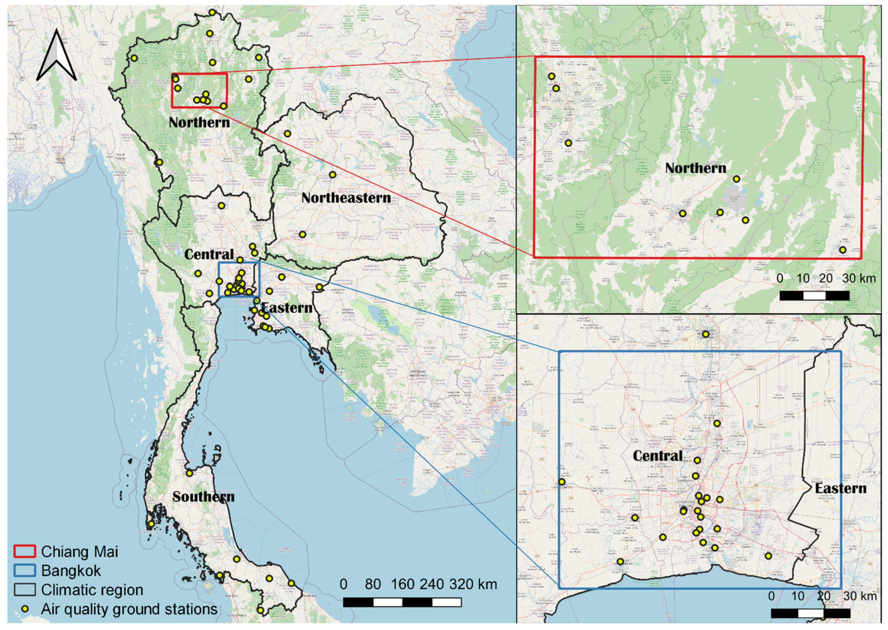
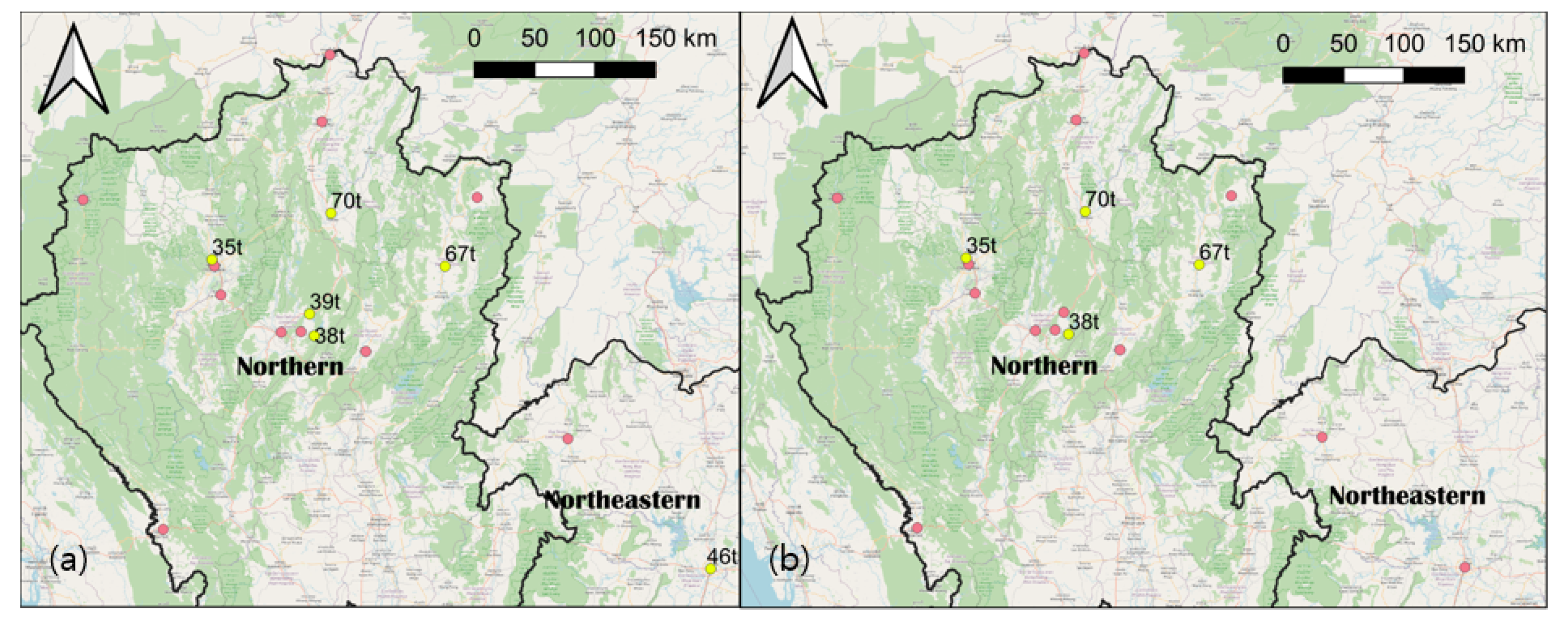
2.1. Study Area
2.2. Data
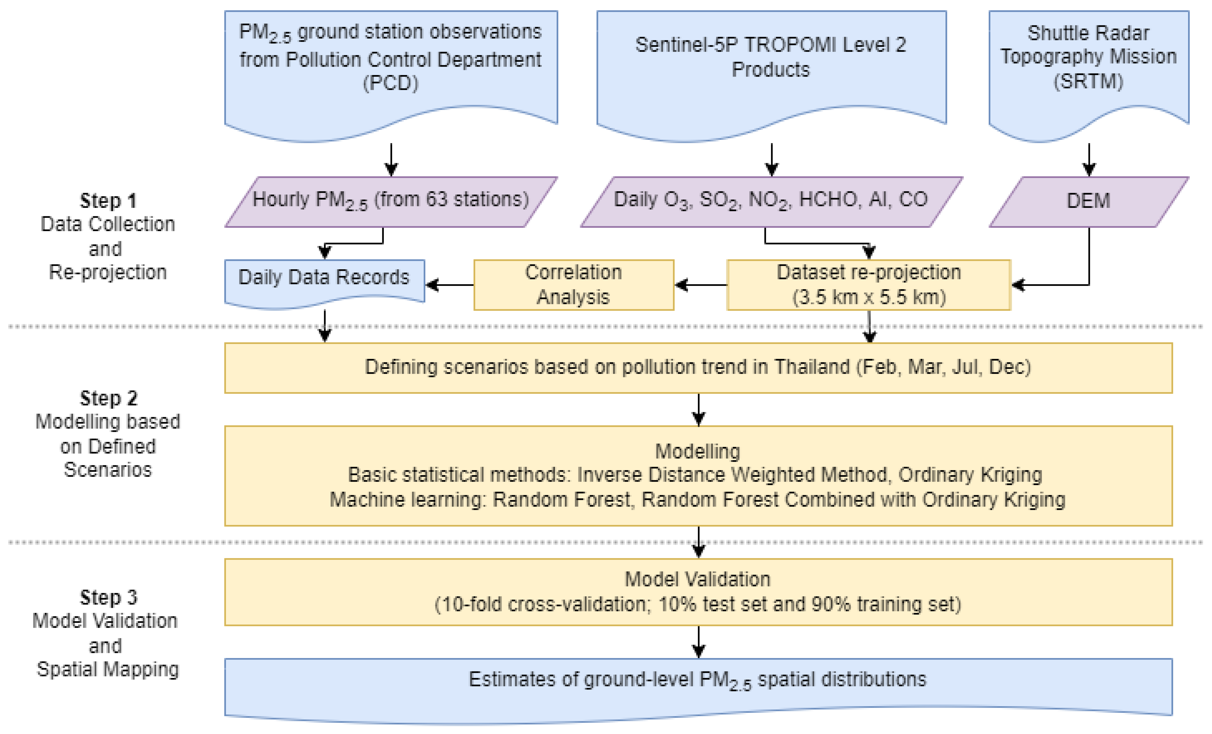
2.3. Methodology
2.3.1. Data Collection and Reprojection
2.3.2. Spatial Interpolation Modeling
2.3.3. Model Validation
3. Results
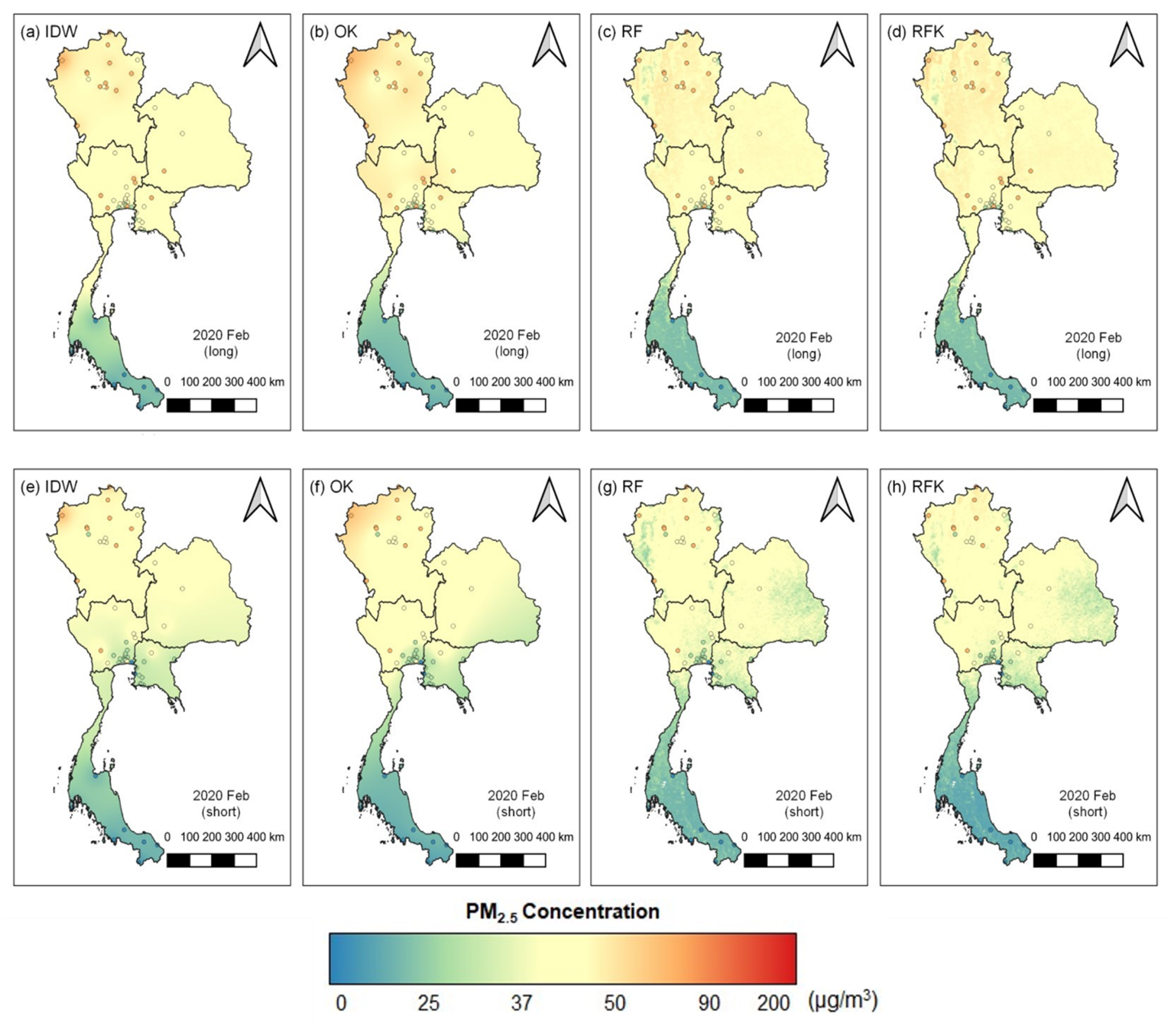
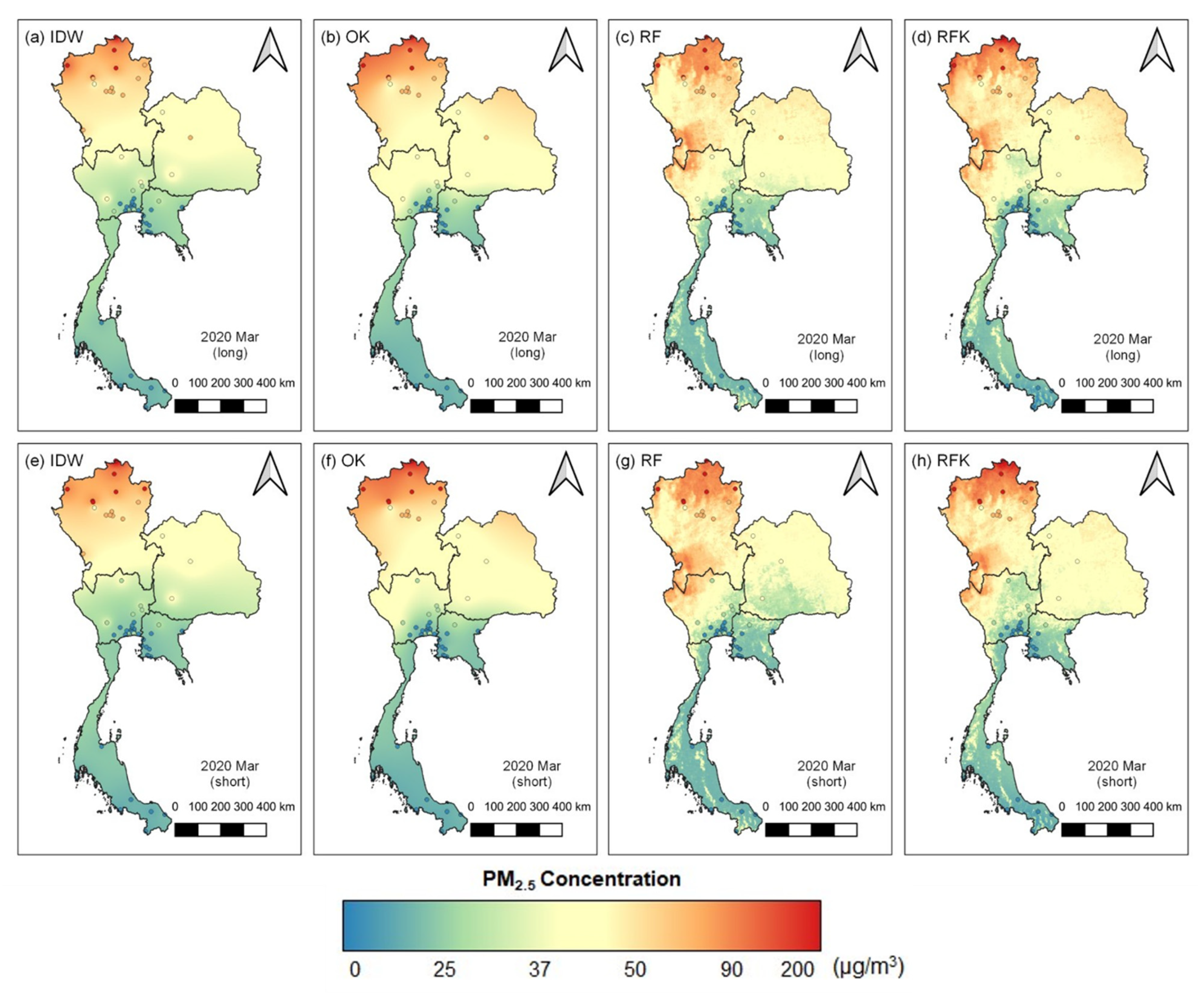
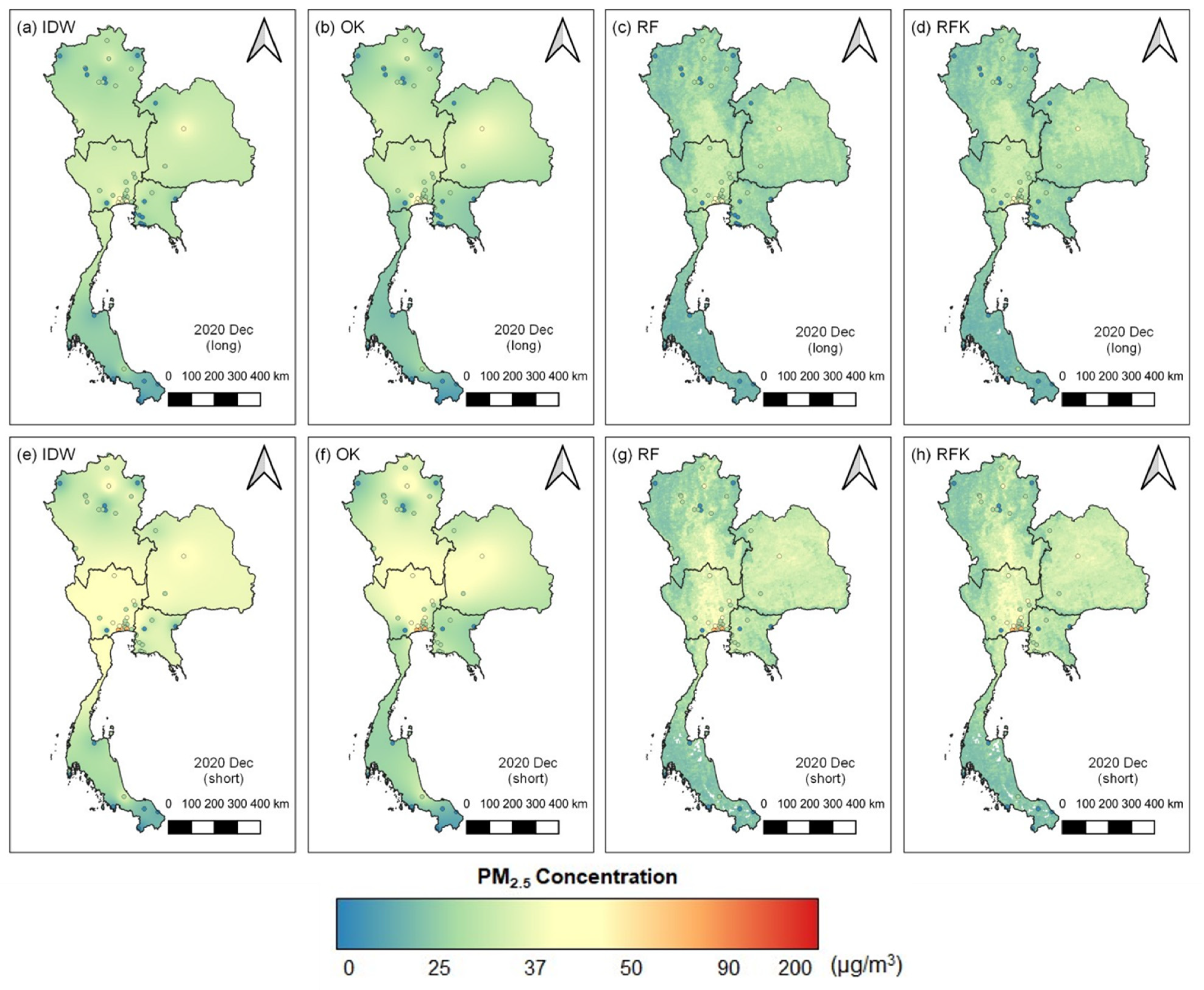
3.1. Spatial Distribution Maps of PM2.5 over Thailand
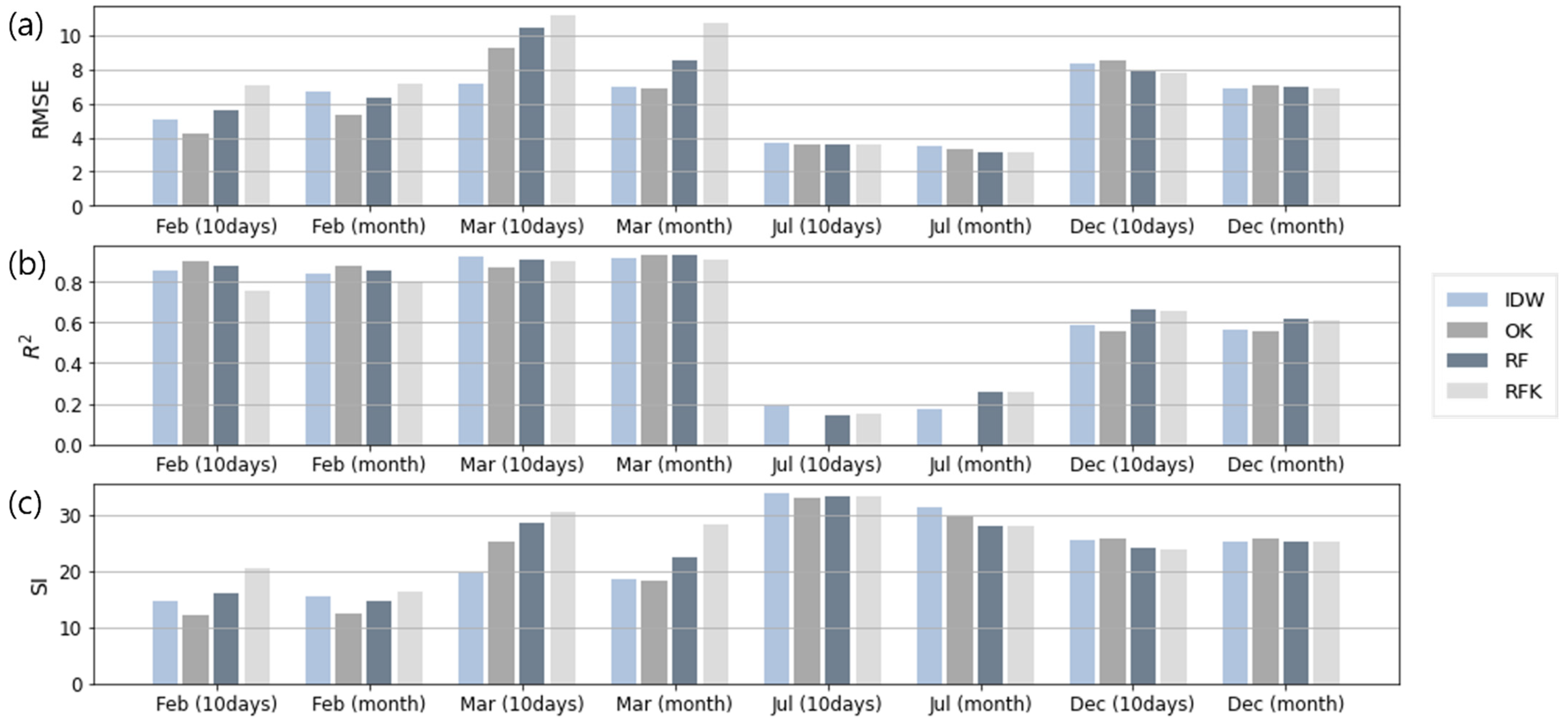
3.2. Ten-Fold Cross-Validation
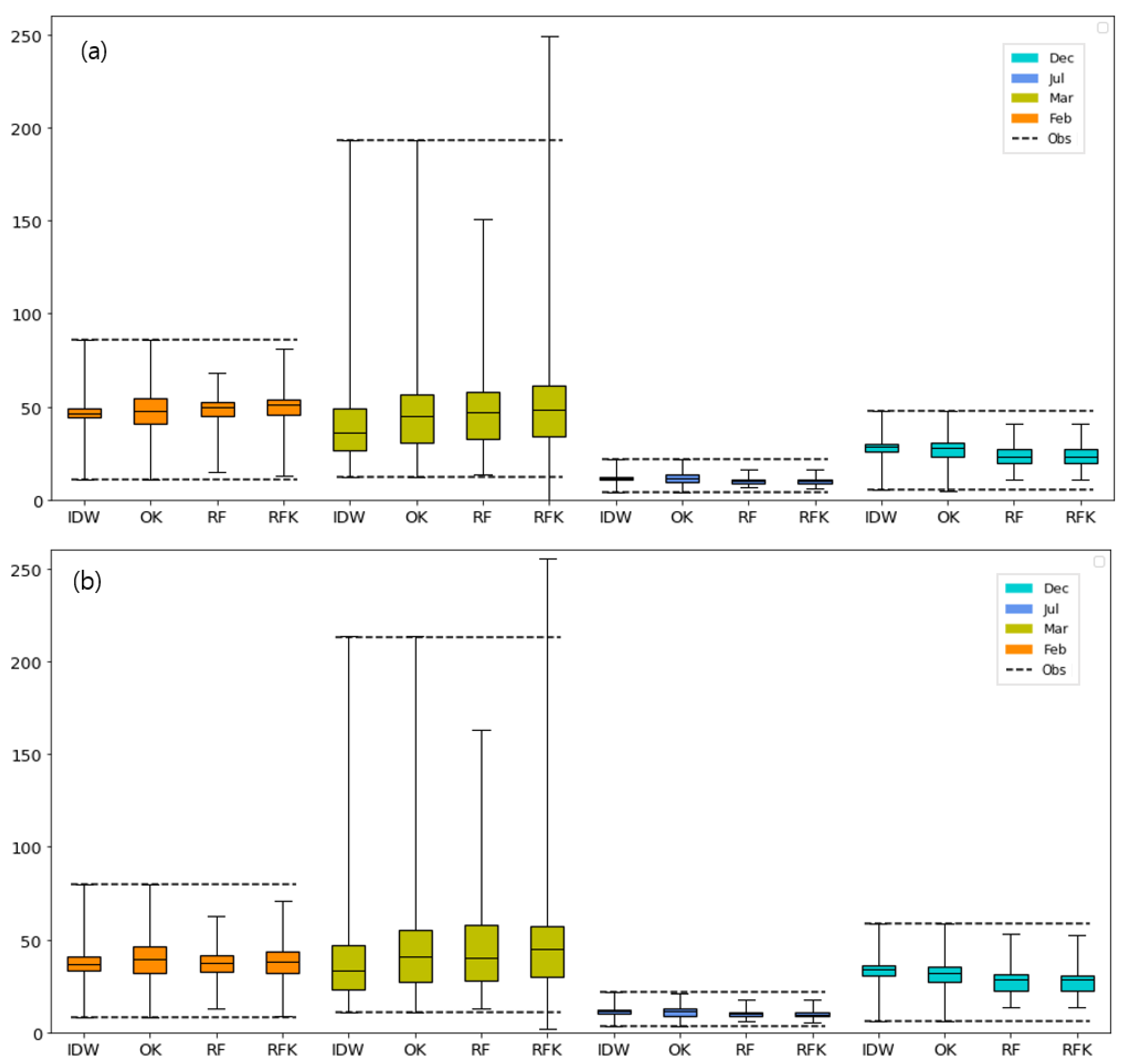
3.3. Data Range of Interpolated Estimates
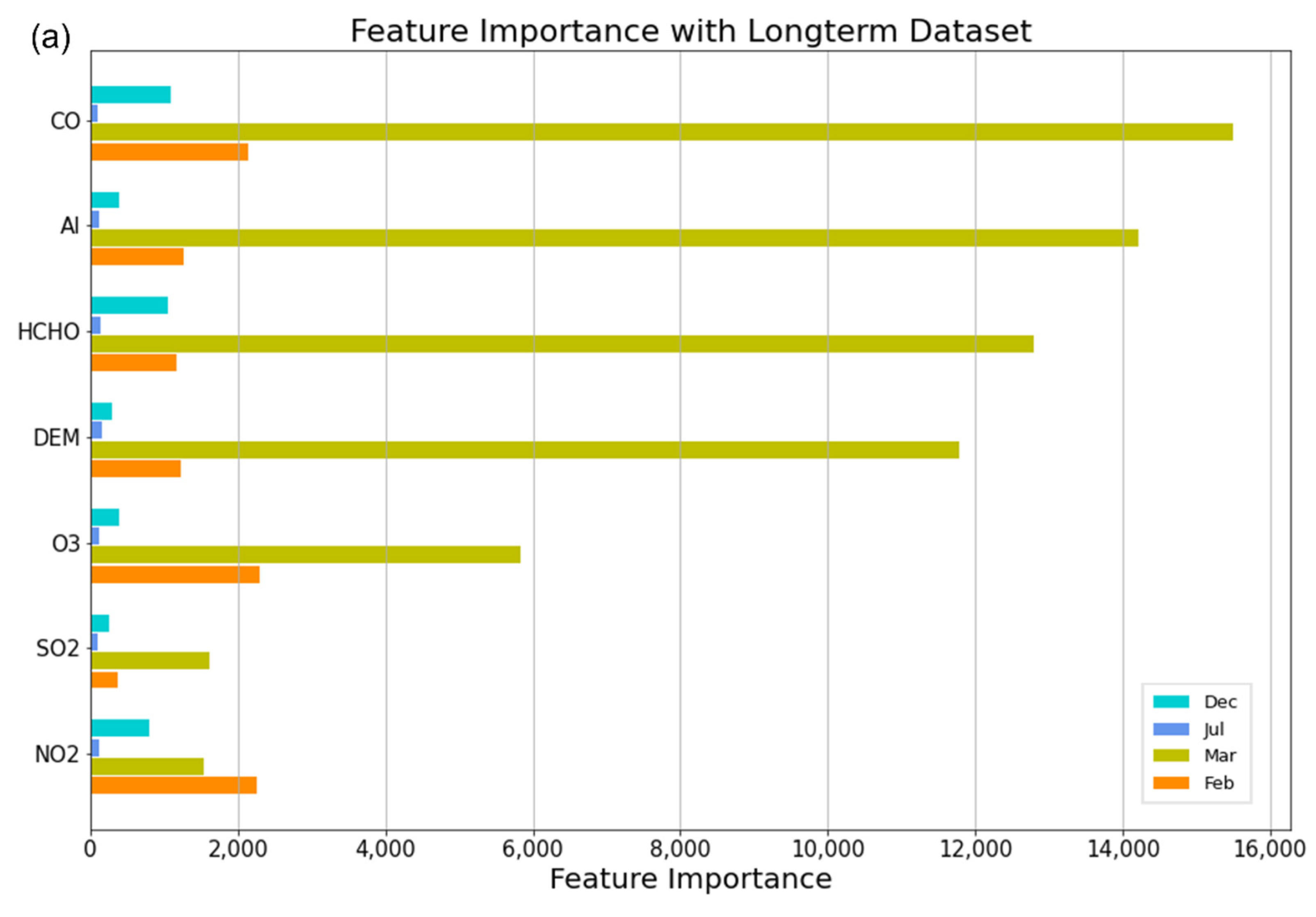
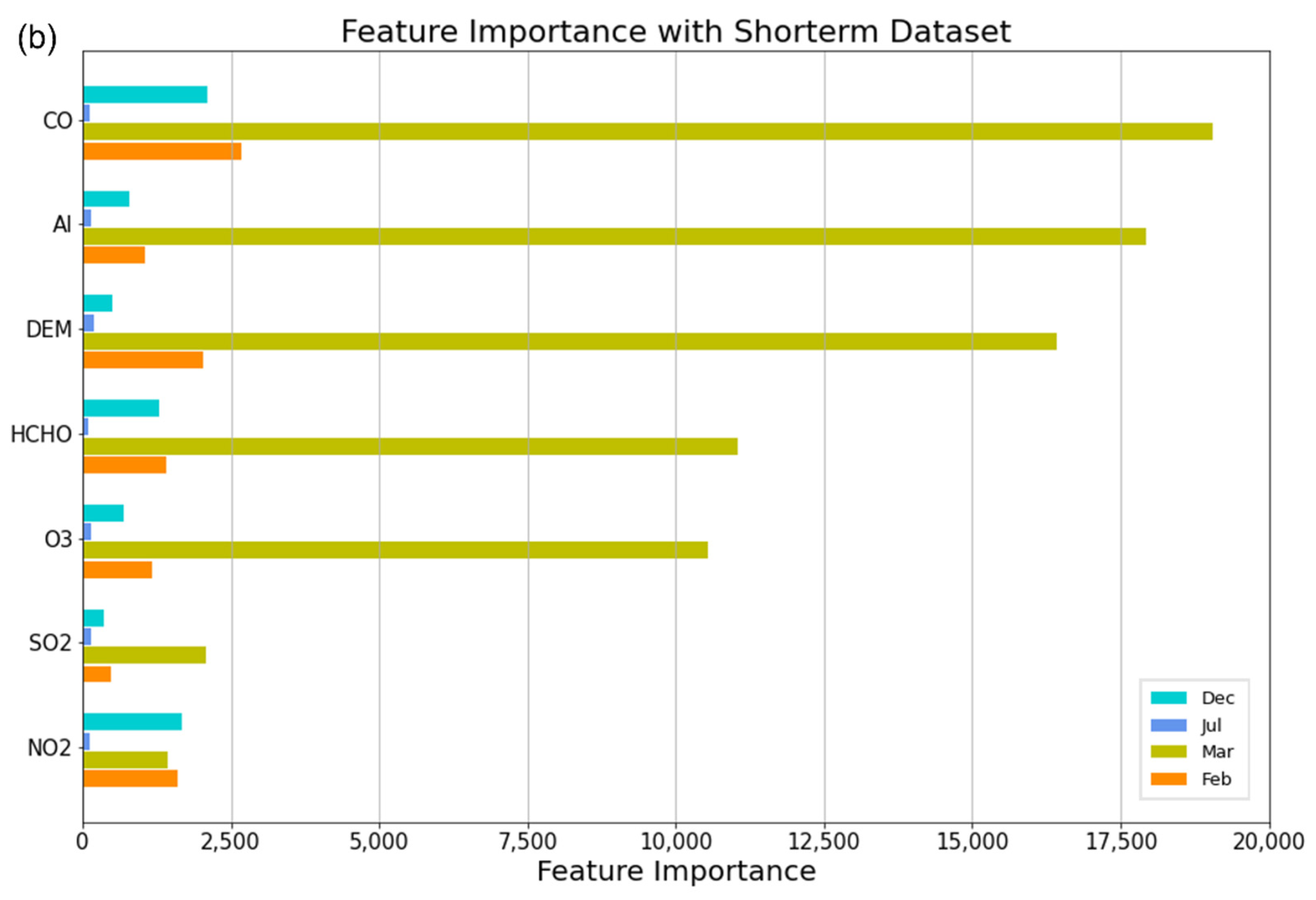
3.4. Analysis of Important Features and Correlation of Covariates
3.5. Station-Based Comparison between Observations and Estimates from Test Sets Observing PM2.5 Concentration Exceeding 50 μg/m3
4. Discussion
5. Summary
Author Contributions
Funding
Data Availability Statement
Acknowledgments
Conflicts of Interest
Abbreviations
| Abbreviation | Definition |
| AI | aerosol index |
| CO | carbon monoxide |
| DEM | digital elevation model |
| GEMS | Global Environmental Monitoring System |
| HCHO | formaldehyde |
| IDW | inverse distance weighted |
| ML | machine learning |
| NASA | National Aeronautics and Space Administration |
| NGA | National Geospatial-Intelligence Agency |
| NWP | numerical weather prediction |
| NO2 | nitrogen dioxide |
| O3 | ozone |
| OK | ordinary kriging |
| PCD | Pollution Control Department |
| PM | particulate matter |
| PM2.5 | particulate matter with an aerodynamic diameter of less than 2.5 μm |
| R2 | coefficient of determination |
| RF | random forest |
| RFK | random forest combined with ordinary kriging |
| RK | regression kriging |
| RMSE | root-mean-squared error |
| Sentinel-5P | Sentinel 5 Precursor |
| SI | scatter index |
| SO2 | sulfur dioxide |
| SRTM | Shuttle Radar Topography Mission |
| SVM | support vector machine |
| TROPOMI | TROPOspheric Monitoring Instrument |
References
- Lee, M.; Lin, L.; Chen, C.Y.; Tsao, Y.; Yao, T.H.; Fei, M.H.; Fang, S.H. Forecasting air quality in Taiwan by using machine learning. Sci. Rep. 2020, 10, 4153. [Google Scholar] [CrossRef]
- Ghorani-Azam, A.; Riahi-Zanjani, B.; Balali-Mood, M. Effects of air pollution on human health and practical measures for prevention in Iran. J. Res. Med. Sci. 2016, 21, 65. [Google Scholar]
- Wang, J.; Ogawa, S. Effects of meteorological conditions on PM2.5 concentrations in Nagasaki, Japan. Int. J. Environ. Res. Public Health 2015, 12, 9089–9101. [Google Scholar] [CrossRef] [PubMed]
- Domingo, J.L.; Marquès, M.; Rovira, J. Influence of airborne transmission of SARS-CoV-2 on COVID-19 pandemic. A review. Environ. Res. 2020, 188, 109861. [Google Scholar] [CrossRef] [PubMed]
- Cazzolla Gatti, R.; Velichevskaya, A.; Tateo, A.; Amoroso, N.; Monaco, A. Machine learning reveals that prolonged exposure to air pollution is associated with SARS-CoV-2 mortality and infectivity in Italy. Environ. Pollut. 2020, 267, 115471. [Google Scholar] [CrossRef]
- Comunian, S.; Dongo, D.; Milani, C.; Palestini, P. Air pollution and COVID-19: The role of particulate matter in the spread and increase of COVID-19’s morbidity and mortality. Int. J. Environ. Res. Public Health 2020, 17, 4487. [Google Scholar] [CrossRef]
- Iskandaryan, D.; Ramos, F.; Trilles, S. Air Quality Prediction in smart cities using machine learning technologies based on sensor data: A Review. Appl. Sci. 2020, 10, 2401. [Google Scholar] [CrossRef] [Green Version]
- Vichit-Vadakan, N.; Vajanapoom, N. Health Impact from Air Pollution in Thailand: Current and Future Challenges. Environ. Health Perspect. 2011, 119, A197. [Google Scholar] [CrossRef] [Green Version]
- Yu, H.; Russell, A.; Mulholland, J.; Odman, T.; Hu, Y.; Chang, H.H.; Kumar, N. Cross-comparison and evaluation of air pollution field estimation methods. Sustain. Cities Soc. 2018, 179, 49–60. [Google Scholar] [CrossRef]
- Chen, L.J.; Ho, Y.H.; Lee, H.C.; Wu, H.C.; Liu, H.M.; Hsieh, H.H.; Huang, Y.; Lung, S.C.C. An open framework for participatory PM2.5 monitoring in smart cities. IEEE Access 2017, 5, 14441–14454. [Google Scholar] [CrossRef]
- Kim, S.; Park, S.; Lee, J. Evaluation of performance of inexpensive laser based PM2.5 sensor monitors for typical indoor and outdoor hotspots of South Korea. Appl. Sci. 2019, 9, 1947. [Google Scholar] [CrossRef] [Green Version]
- Mak, H.W.L.; Lam, Y.F. Comparative assessments and insights of data openness of 50 smart cities in air quality aspects. Sustain. Cities Soc. 2021, 69, 102868. [Google Scholar] [CrossRef]
- Park, S.; Lee, J.; Im, J.; Song, C.K.; Choi, M.; Kim, J.; Lee, S.; Park, R.; Kim, S.M.; Yoon, J.; et al. Estimation of spatially continuous daytime particulate matter concentrations under all sky conditions through the synergistic use of satellite-based AOD and numerical models. Sci. Total Environ. 2020, 713, 136516. [Google Scholar] [CrossRef] [PubMed]
- Janssen, S.; Dumont, G.; Fierens, F.; Mensink, C. Spatial interpolation of air pollution measurements using CORINE land cover data. Atmos. Environ. 2008, 42, 4884–4903. [Google Scholar] [CrossRef]
- Pearce, J.L.; Rathbun, S.L.; Aguilar-Villalobos, M.; Naeher, L.P. Characterizing the spatiotemporal variability of PM2.5 in Cusco, Peru using kriging with external drift. Atmos. Environ. 2009, 43, 2060–2069. [Google Scholar] [CrossRef]
- Li, J.; Heap, A.D. Spatial interpolation methods applied in the environmental sciences: A review. Environ. Model. Softw. 2014, 53, 173–189. [Google Scholar] [CrossRef]
- Karydas, C.G.; Gitas, I.Z.; Koutsogiannaki, E.; Lydakis-Simantiris, N.; Silleos, G.N. Evaluation of spatial interpolation techniques for mapping agricultural topsoil properties in Crete. EARSeL EProceedings 2009, 8, 26–39. [Google Scholar]
- Zhang, G.; Rui, X.; Fan, Y. Critical review of methods to estimate PM2.5 concentrations within specified research region. ISPRS Int. J. Geo Inf. 2018, 7, 368. [Google Scholar] [CrossRef] [Green Version]
- Lu, G.Y.; Wong, D.W. An adaptive inverse-distance weighting spatial interpolation technique. Comput. Geosci. 2008, 34, 1044–1055. [Google Scholar] [CrossRef]
- Kravchenko, A.; Bullock, D.G. A comparative study of interpolation methods for mapping soil properties. Agron. J. 1999, 91, 393–400. [Google Scholar] [CrossRef]
- Deligiorgi, D.; Philippopoulos, K. Spatial interpolation methodologies in urban air pollution modeling: Application for the greater area of metropolitan Athens, Greece. Adv. Air Pollut. 2011, 17, 341–362. [Google Scholar]
- Li, J.; Heap, A.D.; Potter, A.; Daniell, J.J. Application of machine learning methods to spatial interpolation of environmental variables. Environ. Model. Softw. 2011, 26, 1647–1659. [Google Scholar] [CrossRef]
- Chen, P.C.; Lin, Y.T. Exposure assessment of PM2.5 using smart spatial interpolation on regulatory air quality stations with clustering of densely-deployed microsensors. Environ. Pollut. 2021, 292, 118401. [Google Scholar] [CrossRef] [PubMed]
- Wackernagel, H. Multivariate Geostatistics: An Introduction with Applications; Springer: Berlin, Germany, 1998. [Google Scholar]
- Sekulić, A.; Kilibarda, M.; Heuvelink, G.B.M.; Nikolić, M.; Bajat, B. Random forest spatial interpolation. Int. J. Remote Sens. 2020, 12, 1687. [Google Scholar] [CrossRef]
- Hengl, T.; Nussbaum, M.; Wright, M.N.; Heuvelink, G.B.M.; Gräler, B. Random forest as a generic framework for predictive modeling of spatial and spatio-temporal variables. PeerJ. 2018, 8, e5518. [Google Scholar] [CrossRef] [Green Version]
- Bozán, C.; Takács, K.; Körösparti, J.; Laborczi, A.; Túri, N.; Pásztor, L. Integrated spatial assessment of inland excess water hazard on the Great Hungarian Plain. Land Degrad. Dev. 2018, 29, 4373–4386. [Google Scholar] [CrossRef]
- Szatmári, G.; Pásztor, L. Comparison of various uncertainty modelling approaches based on geostatistics and machine learning algorithms. Geoderma 2019, 337, 1329–1340. [Google Scholar] [CrossRef]
- Laborczi, A.; Bozán, C.; Körösparti, J.; Szatmári, G.; Kajári, B.; Túri, N.; Kerezsi, G.; Pásztor, L. Application of Hybrid Prediction Methods in Spatial Assessment of Inland Excess Water Hazard. ISPRS Int. J. Geo Inf. 2020, 9, 268. [Google Scholar] [CrossRef]
- Mammadov, E.; Nowosad, J.; Glaesser, C. Estimation and mapping of surface soil properties in the Caucasus Mountains, Azerbaijan using high-resolution remote sensing data. Geoderma Reg. 2021, 26, e00411. [Google Scholar] [CrossRef]
- Araki, S.; Shima, M.; Yamamoto, K. Spatiotemporal land use random forest model for estimating metropolitan NO2 exposure in Japan. Sci. Total Environ. 2018, 634, 1269–1277. [Google Scholar] [CrossRef]
- Climatological Group; Meteorological Development Bureau; Meteorological Department. The Climate of Thailand. 2015. Available online: https://www.tmd.go.th/en/archive/thailand_climate.pdf (accessed on 20 December 2021).
- Veefkind, J.P.; Aben, I.; McMullan, K.; Förster, H.; de Vries, J.; Otter, G.; Claas, J.; Eskes, H.J.; de Haan, J.F.; Kleipool, Q.; et al. TROPOMI on the ESA Sentinel-5 Precursor: A GMES mission for global observations of the atmospheric composition for climate, air quality and ozone layer applications. Remote Sens. Environ. 2012, 120, 70–83. [Google Scholar] [CrossRef]
- Lary, D.J.; Lary, T.; Sattler, B. Using machine learning to estimate global PM2.5 for environmental health studies. Environ. Health Insights 2020, 9s1, EHI-S15664. [Google Scholar] [CrossRef]
- Lary, D.J.; Faruque, F.S.; Malakar, N.; Moore, A.; Roscoe, B.; Adams, Z.L.; Eggelston, Y. Estimating the global abundance of ground level presence of particulate matter (PM2.5). Geospat. Health 2014, 8, S611–S630. [Google Scholar] [CrossRef] [PubMed]
- Schulte, N.; Li, X.; Ghosh, J.K.; Fine, P.M.; Epstein, S.A. Responsive high-resolution air quality index mapping using model, regulatory monitor, and sensor data in real-time. Environ. Res. Lett. 2020, 15, 1040a7. [Google Scholar] [CrossRef]
- Theys, N.; de Smedt, I.; Yu, H.; Danckaert, T.; van Gent, J.; Hörmann, C.; Wagner, T.; Hedelt, P.; Bauer, H.; Romahn, F.; et al. Sulfur dioxide retrievals from TROPOMI onboard Sentinel-5 Precursor: Algorithm theoretical basis. Atmos. Meas. Tech. 2017, 10, 119–153. [Google Scholar] [CrossRef] [Green Version]
- Sharma, S.; Zhang, M.; Anshika; Gao, J.; Zhang, H.; Kota, S.H. Effect of restricted emissions during COVID-19 on air quality in India. Sci. Total Environ. 2020, 728, 138878. [Google Scholar] [CrossRef] [PubMed]
- Stratoulias, D.; Nuthammachot, N. Air quality development during the COVID-19 pandemic over a medium-sized urban area in Thailand. Sci. Total Environ. 2020, 746, 141320. [Google Scholar] [CrossRef]
- Fan, C.; Li, Y.; Guang, J.; Li, Z.; Elnashar, A.; Allam, M.; de Leeuw, G. The impact of the control measures during the COVID-19 outbreak on air pollution in China. Int. J. Remote Sens. 2020, 12, 1613. [Google Scholar] [CrossRef]
- Bauwens, M.; Compernolle, S.; Stavrakou, T.; Müller, J.-F.; van Gent, J.; Eskes, H.; Levelt, P.F.; van der A, R.; Veefkind, J.P.; Vlietinck, J.; et al. Impact of coronavirus outbreak on NO2 pollution assessed using TROPOMI and OMI observations. Geophys. Res. Lett. 2020, 47, e2020GL087978. [Google Scholar] [CrossRef]
- Gitahi, J.; Hahn, M.; Ramirez, A. High-resolution urban air quality monitoring using sentinel satellite images and low-cost ground-based sensor networks. E3S Web Conf. 2020, 3, 102–111. [Google Scholar] [CrossRef]
- Wang, Y.; Wang, M.; Huang, B.; Li, S.; Lin, Y. Estimation and analysis of the nighttime PM2.5 concentration based on LJ1-01 images: A case study in the Pearl River Delta urban agglomeration of China. Remote Sens. 2021, 13, 3405. [Google Scholar] [CrossRef]
- Wei, J.; Li, Z.; Cribb, M.; Huang, W.; Xue, W.; Sun, L.; Guo, J.; Peng, Y.; Li, J.; Lyapustin, A.; et al. Improved 1 km resolution PM2.5 estimates across China using enhanced space-time extremely randomized trees. Atmos. Chem. Phys. 2020, 20, 3273–3289. [Google Scholar] [CrossRef] [Green Version]
- Choi, W.; Lee, H.; Kim, D.; Kim, S. Improving spatial coverage of satellite aerosol classification using a random forest model. Remote Sens. 2021, 13, 1268. [Google Scholar] [CrossRef]
- Li, T.; Wang, Y.; Yuan, Q. Remote sensing estimation of regional NO2 via space-time neural networks. Remote Sens. 2020, 12, 2514. [Google Scholar] [CrossRef]
- Wang, Y.; Yuan, Q.; Li, T.; Tan, S.; Zhang, L. Full-coverage spatiotemporal mapping of ambient PM2.5 and PM10 over China from Sentinel-5P and assimilated datasets: Considering the precursors and chemical compositions. Sci. Total Environ. 2021, 793, 148535. [Google Scholar] [CrossRef] [PubMed]
- Zhou, L.; Zhou, C.; Yang, F.; Che, L.; Wang, B.; Sun, D. Spatio-temporal evolution and the influencing factors of PM2.5 in China between 2000 and 2015. J. Geogr. Sci. 2019, 29, 253–270. [Google Scholar] [CrossRef] [Green Version]
- Huang, R.J.; Zhang, Y.; Bozzetti, C.; Ho, K.F.; Cao, J.J.; Han, Y.; Daellenbach, K.R.; Slowik, J.G.; Platt, S.M.; Canonaco, F.; et al. High secondary aerosol contribution to particulate pollution during haze events in China. Nature 2014, 514, 218–222. [Google Scholar] [CrossRef] [PubMed] [Green Version]
- Luecken, D.J.; Napelenok, S.L.; Strum, M.; Scheffe, R.; Phillips, S. Sensitivity of ambient atmospheric formaldehyde and ozone to precursor species and source types across the U.S. J. Environ. Sci. Technol. 2018, 52, 4668. [Google Scholar] [CrossRef] [PubMed]
- Fu, H.; Zhang, Y.; Liao, C.; Mao, L.; Wang, Z.; Hong, N. Investigating PM2.5 responses to other air pollutants and meteorological factors across multiple temporal scales. Sci. Rep. 2020, 10, 15639. [Google Scholar] [CrossRef]
- Liu, X.; Pan, X.; Wang, Z.; He, H.; Wang, D.; Liu, H.; Tian, Y.; Xiang, W.; Li, J. Chemical characteristics and potential sources of PM2.5 in Shahe city during severe haze pollution episodes in the winter. Aerosol Air Qual. Res. 2020, 20, 2741–2753. [Google Scholar] [CrossRef]
- Eskes, H.J.; Eichmann, K.U. S5P MPC Product Readme Nitrogen Dioxide; 2019; 1.5, S5P-MPC-KNMI-RPF-NO2. Available online: http://www.tropomi.eu/sites/default/files/files/publicSentinel-5P-Nitrogen-Dioxide-Level-2-Product-Readme-File_20191105.pdf (accessed on 21 November 2021).
- Eatough, D.J.; Caka, F.M.; Farber, R.J. The conversion of SO2 to sulfate in the atmosphere. Isr. J. Chem. 1994, 34, 301–314. [Google Scholar] [CrossRef]
- Khoder, M.I. Atmospheric conversion of sulfur dioxide to particulate sulfate and nitrogen dioxide to particulate nitrate and gaseous nitric acid in an urban area. Chemosphere 2002, 49, 675–684. [Google Scholar] [CrossRef]
- Zhu, J.; Chen, L.; Liao, H.; Dang, R. Correlations between PM2.5 and Ozone over China and Associated Underlying Reasons. Atmosphere 2019, 10, 352. [Google Scholar] [CrossRef] [Green Version]
- Di, Q.; Kloog, I.; Koutrakis, P.; Lyapustin, A.; Wang, Y.; Schwartz, J. Assessing PM2.5 Exposures with High Spatiotemporal Resolution across the Continental United States. Environ. Sci. Technol. 2016, 50, 4712–4721. [Google Scholar] [CrossRef] [PubMed] [Green Version]
- Zweers, S. TROPOMI ATBD of the UV Aerosol Index; 2021; 2.0, S5P-KNMI-L2-0008-RP. Available online: https://sentinel.esa.int/documents/247904/2476257/Sentinel-5P-TROPOMI-ATBD-UV-Aerosol-Index (accessed on 21 November 2021).
- Sritong-aon, C.; Thomya, J.; Kertpromphan, C.; Phosri, A. Estimated effects of meteorological factors and fire hotspots on ambient particulate matter in the northern region of Thailand. Air Qual. Atmos. Health 2021, 14, 1857–1868. [Google Scholar] [CrossRef]
- Weichenthal, S.; Kulka, R.; Lavigne, E.; van Rijswijk, D.; Brauer, M.; Villeneuve, P.J.; Stieb, D.; Joseph, L.; Burnett, R.T. Biomass Burning as a Source of Ambient Fine Particulate Air Pollution and Acute Myocardial Infarction. Int. J. Epidemiol. 2017, 28, 329–337. [Google Scholar] [CrossRef] [Green Version]
- Roberts, E.A.; Sheley, R.L.; Lawrence, R.L. Using sampling and inverse distance weighted modeling for Using sampling and inverse distance weighted modeling for mapping invasive plants mapping invasive plants. West. N. Am. Nat. 2004, 64, 8–27. [Google Scholar]
- Cressie, N. Geostatistics. Am. Stat. 1989, 43, 197–202. [Google Scholar]
- Schneider, R.; Vicedo-Cabrera, A.M.; Sera, F.; Masselot, P.; Stafoggia, M.; de Hoogh, K.; Kloog, I.; Reis, S.; Vieno, M.; Gasparrini, A. A satellite-based spatio-temporal machine learning model to reconstruct daily PM2.5 concentrations across Great Britain. Int. J. Remote Sens. 2020, 12, 3803. [Google Scholar] [CrossRef] [PubMed]
- Jiang, T.; Chen, B.; Nie, Z.; Ren, Z.; Xu, B.; Tang, S. Estimation of hourly full-coverage PM2.5 concentrations at 1-km resolution in China using a two-stage random forest model. Atmos. Res. 2021, 248, 105146. [Google Scholar] [CrossRef]
- Jung, C.R.; Chen, W.T.; Nakayama, S.F. A national-scale 1-km resolution PM2.5 estimation model over japan using maiac aod and a two-stage random forest model. Remote Sens. 2021, 13, 3657. [Google Scholar] [CrossRef]
- Zhang, T.; He, W.; Zheng, H.; Cui, Y.; Song, H.; Fu, S. Satellite-based ground PM2.5 estimation using a gradient boosting decision tree. Chemosphere 2021, 268, 128801. [Google Scholar] [CrossRef]
- R Core Team. R: The R Project for Statistical Computing. 2020. Available online: https://www.r-project.org/ (accessed on 7 January 2022).
- Lee, C.; Lee, K.; Kim, S.; Yu, J.; Jeong, S.; Yeom, J. Hourly ground-level PM2.5 estimation using geostationary satellite and reanalysis data via deep learning. Int. J. Remote Sens. 2021, 13, 2121. [Google Scholar] [CrossRef]
- Shen, H.; Li, T.; Yuan, Q.; Zhang, L. Estimating regional ground-level PM2.5 directly from satellite top-of-atmosphere reflectance using deep belief networks. J. Geophys Res. Atmos. 2018, 123, 13875–13886. [Google Scholar] [CrossRef] [Green Version]
- Di, Q.; Amini, H.; Shi, L.; Kloog, I.; Silvern, R.; Kelly, J.; Sabath, M.B.; Choirat, C.; Koutrakis, P.; Lyapustin, A.; et al. An ensemble-based model of PM2.5 concentration across the contiguous United States with high spatiotemporal resolution. Environ. Int. 2019, 130, 104909. [Google Scholar] [CrossRef]
- Sajjadi, S.A.; Zolfaghari, G.; Adab, H.; Allahabadi, A.; Delsouz, M. Measurement and modeling of particulate matter concentrations: Applying spatial analysis and regression techniques to assess air quality. MethodsX 2017, 4, 372–390. [Google Scholar] [CrossRef] [PubMed]
- Zou, B.; Luo, Y.; Wan, N.; Zheng, Z.; Sternberg, T.; Liao, Y. Performance comparison of LUR and OK in PM2.5 concentration mapping: A multidimensional perspective. Sci. Rep. 2015, 5, 8698. [Google Scholar] [CrossRef] [Green Version]
- Guo, B.; Zhang, D.; Pei, L.; Su, Y.; Wang, X.; Bian, Y.; Zhang, D.; Yao, W.; Zhou, Z.; Guo, L. Estimating PM2.5 concentrations via random forest method using satellite, auxiliary, and ground-level station dataset at multiple temporal scales across China in 2017. Sci. Total Environ. 2021, 778, 146288. [Google Scholar] [CrossRef] [PubMed]
- Liang, F.; Xiao, Q.; Huang, K.; Yang, X.; Liu, F.; Li, J.; Lu, X.; Liu, Y.; Gu, D. The 17-y spatiotemporal trend of PM2.5 and its mortality burden in China. Proc. Natl. Acad. Sci. USA 2020, 117, 25601–25608. [Google Scholar] [CrossRef]
- Meng, X.; Liu, C.; Zhang, L.; Wang, W.; Stowell, J.; Kan, H.; Liu, Y. Estimating PM2.5 concentrations in Northeastern China with full spatiotemporal coverage, 2005–2016. Remote Sens. Environ. 2021, 253, 112203. [Google Scholar] [CrossRef]


| Northern Region | Northeastern Region | Central Region | Eastern Region | Southern Region | |
|---|---|---|---|---|---|
| Number of provinces | 15 | 20 | 18 | 8 | 10 |
| Prevalent topography | mountainous | A high-level plateau | A low-level plain | Plains and valleys | Peninsula |
| Average surface temperature * (°C) | 23.4/28.1/27.3 | 24.2/28.6/27.6 | 26.2/29.7/28.2 | 26.7/29.1/28.3 | 26.3/28.2/27.8 |
| Precipitation * (mm) | 100.4/187.3/943.2 | 76.3/224.4/1103.8 | 127.3/205.4/942.5 | 178.4/277.3/1433.2 | 827.9/229.0/680.0 |
| Relative Humidity * (%) | 74/63/81 | 69/66/80 | 70/68/78 | 71/75/81 | 81/78/79 |
| PCD | Sentinel-5P | SRTM | |||||
|---|---|---|---|---|---|---|---|
| Correlation with PM2.5 | O3 | SO2 | NO2 | HCHO | AI | CO | DEM |
| 8 February–18 February | 0.56 *** | 0.09 ns | −0.09 ns | 0.62 *** | 0.49 *** | 0.74 *** | 0.53 *** |
| 1 February–29 February | 0.72 *** | 0.08 ns | 0.10 ns | 0.67 *** | 0.43 *** | 0.72 *** | 0.35 ** |
| 19 March–29 March | 0.36 ** | 0.22 ns | 0.10 ns | 0.79 *** | 0.88 *** | 0.89 *** | 0.73 *** |
| 1 March–31 March | 0.34 ** | 0.28 ns | −0.04 ns | 0.79 *** | 0.87 *** | 0.87 *** | 0.72 *** |
| 9 July–19 July | 0.16 ns | −0.20 ns | 0.24 * | 0.16 ns | 0.27 * | 0 ns | −0.34 ** |
| 1 July–30 July | 0.08 ns | 0.02 ns | 0.24 * | 0.21 ns | 0.26 * | −0.15 ns | −0.33 ** |
| 5 December–15 December | −0.04 ns | 0 ns | 0.63 *** | 0.65 *** | 0.64 *** | 0.75 *** | −0.30 * |
| 1 December–31 December | −0.20 ns | 0.12 ns | 0.61 *** | 0.76 *** | 0.49 *** | 0.74 *** | −0.26 * |
| March (Monthly) | IDW | OK | RF | RFK | |||||
|---|---|---|---|---|---|---|---|---|---|
| Station ID | Obs. | Est. | Error Rate (%) | Est. | Error Rate (%) | Est. | Error Rate (%) | Est. | Error Rate (%) |
| 39t | 56.590 | 59.618 | 5.350 | 61.296 | 8.316 | 67.097 | 18.567 | 58.073 | 2.620 |
| 70t | 94.528 | 75.322 | −20.318 | 83.495 | −11.672 | 115.955 | 22.667 | 82.959 | −12.239 |
| 67t | 68.601 | 71.376 | 4.045 | 73.554 | 7.220 | 75.356 | 9.846 | 88.475 | 28.970 |
| 46t | 50.302 | 38.427 | −23.607 | 43.719 | −13.086 | 53.699 | 6.754 | 55.668 | 10.667 |
| 35t | 91.029 | 79.408 | −12.766 | 83.815 | −7.925 | 83.575 | −8.189 | 87.761 | −3.590 |
| 38t | 56.961 | 58.294 | 2.341 | 60.105 | 5.521 | 71.671 | 25.826 | 56.987 | 0.047 |
| Average RMSE | 10.51646 | 6.753721 | 12.23814 | 9.750932 | |||||
| March (10-Day) | IDW | OK | RF | RFK | |||||
|---|---|---|---|---|---|---|---|---|---|
| Station ID | Obs. | Est. | Error Rate (%) | Est. | Error Rate (%) | Est. | Error Rate (%) | Est. | Error Rate (%) |
| 39t | 60.631 | 62.802 | 3.580 | 65.054 | 7.295 | 78.084 | 28.786 | 66.182 | 9.156 |
| 70t | 95.967 | 80.808 | −15.796 | 92.471 | −3.642 | 120.197 | 25.249 | 115.140 | 19.979 |
| 67t | 69.676 | 74.421 | 6.810 | 73.792 | 5.906 | 80.126 | 14.997 | 82.751 | 18.764 |
| 46t | 50.302 | 38.427 | −23.607 | 43.719 | −13.086 | 53.699 | 6.754 | 55.668 | 10.667 |
| 35t | 114.466 | 93.681 | −18.158 | 89.176 | −22.095 | 91.627 | −19.953 | 108.798 | −4.952 |
| 38t | 60.884 | 61.079 | 0.321 | 57.831 | −5.014 | 71.236 | 17.003 | 61.102 | 0.358 |
| Average RMSE | 11.76217 | 11.11301 | 16.53919 | 10.24966 | |||||
| February (Monthly) | IDW | OK | RF | RFK | |||||
|---|---|---|---|---|---|---|---|---|---|
| Station ID | Obs. | Est. | Error Rate (%) | Est. | Error Rate (%) | Est. | Error Rate (%) | Est. | Error Rate (%) |
| 70t | 60.775 | 52.245 | −14.035 | 51.691 | −14.947 | 55.539 | −8.616 | 64.708 | 6.471 |
| 67t | 57.262 | 51.190 | −10.605 | 51.095 | −10.771 | 59.107 | 3.221 | 64.708 | 13.003 |
| 35t | 55.991 | 53.350 | −4.717 | 54.028 | −3.506 | 53.869 | −3.791 | 53.898 | −3.738 |
| 38t | 51.162 | 50.028 | −2.218 | 52.585 | 2.781 | 51.488 | 0.636 | 52.155 | 1.940 |
| Average RMSE | 5.429112 | 5.622299 | 2.976325 | 4.366747 | |||||
| February (10-Day) | IDW | OK | RF | RFK | |||||
|---|---|---|---|---|---|---|---|---|---|
| Station ID | Obs. | Est. | Error Rate (%) | Est. | Error Rate (%) | Est. | Error Rate (%) | Est. | Error Rate (%) |
| 70t | 52.716 | 47.757 | −9.407 | 49.715 | −5.693 | 54.308 | 3.019 | 53.894 | 2.235 |
| 67t | 50.563 | 45.326 | −10.358 | 45.055 | −10.893 | 50.778 | 0.426 | 55.477 | 9.719 |
| 35t | 53.473 | 55.100 | 3.041 | 54.184 | 1.329 | 54.807 | 2.494 | 59.639 | 11.530 |
| 38t | 51.162 | 50.028 | −2.218 | 52.585 | 2.781 | 51.488 | 0.636 | 52.155 | 1.940 |
| Average RMSE | 3.477375 | 3.678844 | 0.882139 | 4.722686 | |||||
Publisher’s Note: MDPI stays neutral with regard to jurisdictional claims in published maps and institutional affiliations. |
© 2022 by the authors. Licensee MDPI, Basel, Switzerland. This article is an open access article distributed under the terms and conditions of the Creative Commons Attribution (CC BY) license (https://creativecommons.org/licenses/by/4.0/).
Share and Cite
Han, S.; Kundhikanjana, W.; Towashiraporn, P.; Stratoulias, D. Interpolation-Based Fusion of Sentinel-5P, SRTM, and Regulatory-Grade Ground Stations Data for Producing Spatially Continuous Maps of PM2.5 Concentrations Nationwide over Thailand. Atmosphere 2022, 13, 161. https://doi.org/10.3390/atmos13020161
Han S, Kundhikanjana W, Towashiraporn P, Stratoulias D. Interpolation-Based Fusion of Sentinel-5P, SRTM, and Regulatory-Grade Ground Stations Data for Producing Spatially Continuous Maps of PM2.5 Concentrations Nationwide over Thailand. Atmosphere. 2022; 13(2):161. https://doi.org/10.3390/atmos13020161
Chicago/Turabian StyleHan, Shinhye, Worasom Kundhikanjana, Peeranan Towashiraporn, and Dimitris Stratoulias. 2022. "Interpolation-Based Fusion of Sentinel-5P, SRTM, and Regulatory-Grade Ground Stations Data for Producing Spatially Continuous Maps of PM2.5 Concentrations Nationwide over Thailand" Atmosphere 13, no. 2: 161. https://doi.org/10.3390/atmos13020161
APA StyleHan, S., Kundhikanjana, W., Towashiraporn, P., & Stratoulias, D. (2022). Interpolation-Based Fusion of Sentinel-5P, SRTM, and Regulatory-Grade Ground Stations Data for Producing Spatially Continuous Maps of PM2.5 Concentrations Nationwide over Thailand. Atmosphere, 13(2), 161. https://doi.org/10.3390/atmos13020161