Long-Term Changes in Ionospheric Climate in Terms of foF2

Abstract

There is not only space weather; there is also space climate. Space climate includes the ionospheric climate, which is affected by long-term trends in the ionosphere. One of the most important ionospheric parameters is the critical frequency of the ionospheric F2 layer, foF2, which corresponds to the maximum ionospheric electron density, NmF2. Observational data series of foF2 have been collected at some stations for as long as over 60 years and continents are relatively well covered by a network of ionosondes, instruments that measure, among others, foF2. Trends in foF2 are relatively weak. The main global driver of long-term trends in foF2 is the increasing concentration of greenhouse gases, namely CO₂, in the atmosphere. The impact of the other important trend driver, the secular change in the Earth’s main magnetic field, is very regional, being positive in some regions, negative in others, and neither in the rest. There are various sources of uncertainty in foF2 trends. One is the inhomogeneity of long foF2 data series. The main driver of year-to-year changes in foF2 is the quasi-eleven-year solar cycle. The removal of its effect is another source of uncertainty. Different methods might provide somewhat different strengths among trends in foF2. All this is briefly reviewed in the paper.

1. Introduction

The background of space weather is formed by space climate, including the ionospheric climate. Changes in the ionospheric climate are affected by long-term changes in solar ionizing radiation (solar activity) and solar wind (represented by geomagnetic activity), by natural and anthropogenic long-term changes in the Earth’s atmosphere, and by long-term (secular) changes in the main magnetic field of the Earth. Whereas natural processes long-term changes are long-term quasi-periodic variations, anthropogenic changes in the atmosphere represent a continuous long-term trend caused by the continuously increasing atmospheric concentration of greenhouse gases, particularly CO₂. This trend is the main focus of this paper.

The critical frequency of the F2 layer of the ionosphere, foF2, corresponds to the electron density maximum in the ionosphere, NmF2, at the vertical radio wave incidence in the ionosphere. Therefore, foF2/NmF2 is a very important parameter for describing the immediate state as well as the climate of the ionosphere. This fact and the availability of long data series from global continents are the reasons why it is the most studied ionospheric parameter in terms of long-term trends (e.g., [1,2,3,4,5,6,7,8,9,10,11,12,13,14,15,16,17,18,19,20,21,22,23,24,25,26,27,28]).

Long-term trends and climate change in the thermosphere and ionosphere are primarily caused by the increasing atmospheric concentration of CO₂ (e.g., [29]). It acts through “greenhouse cooling”, which affects thermospheric and ionospheric chemistry, affecting ionization and recombination processes, and causes thermal shrinking of the thermosphere, thereby changing the height profile of the ionosphere. Direct measurements at heights of 0–110 km reveal an almost height-independent trend in the increase in CO₂ concentration by about 5%/decade, at all heights [30]. Why thermospheric greenhouse cooling and not warming, as in the troposphere? Because atmospheric neutral density decreases as the height increases and, starting from the stratosphere, the CO₂ concentration is so low that it is unable to sufficiently trap the outgoing low frequency radiation (this trapping heats the troposphere) and its second characteristic the strong infrared radiation, which cools the atmosphere, dominates.

It has been recognized that on regional scales, the Earth’s changing main magnetic field also plays an important role in long-term trends in the ionosphere [7,16,31]. A role might also be played by long-term changes in geomagnetic activity. A specific example is the possible impact of long-term (substantially longer than the 11 year cycle) changes in solar activity. The long-term changes in the ionosphere and thermosphere might be also affected by changes in atmospheric waves coming from below, from the lower atmosphere. However, their effects are little known and understood. In the mesosphere and lower thermosphere, these effects appear to be regionally remarkably different (e.g., [29,32,33]).

Section 2 deals with long-term trends in foF2 themselves. Section 3 treats the role of non-CO₂ sources of trends in foF2. Section 4 analyses sources of uncertainty in calculating foF2 trends. Section 5 contains conclusions.

2. Long-Term Trends in foF2

Many papers deal with trends in foF2; some of them are referred to in Section 1, Introduction. It does not make sense to deal with all of them; only some results representing current knowledge and understanding of foF2 trends are presented here. Trends in foF2 were reviewed by [34] and partly by [29,33].

An analysis of the data from 31 European ionosondes revealed negative trends in fof2 west of 30° E but dominant positive trends east of 30° E [2]. A comparison of the trend results obtained by various teams and methods of those times for Juliusruh station (northernmost Germany) over the period 1976–1996 showed that the results of most teams agreed each other and that the trend was weak, about 0.1 MHz/decade [18]. Global foF2 trends were found to be small and not significantly different from zero [20], based on a homogenized data base of monthly means of foF2 [35]. An analysis of a 70 year-long series of observations of ionosonde at Wuhan (30° N, central China) found a weak but statistically significant negative trend in foF2 [36]. At high latitudes, a negative trend in foF2 was found for both hemispheres [1]. At low latitudes, a small and statistically insignificant positive trend in foF2 was found for Ahmedabad in central India [5]. An analysis of a set of 31 ionospheric stations from high, middle, and low latitudes revealed trends in foF2 between +0.7 and −0.6 MHz over 34 years since 1957 [26].

The extreme solar activity minimum in 2008–2009 was expected to exert some impact on trend estimations. However, if the data series of foF2 ended well after 2008–2009, no detectable impact on trends was found [37]. An examination of stability in trends in foF2 using data from Slough/Chilton (England) and Kokobunji (Japan) revealed that foF2 trends become unstable in solar cycle 23, changing when one more year was added [38]. Variations in foF2 trends in solar cycle 23 were attributed to changes in the EUV-F10.7 relation [38].

Trends in foF2 have mostly been studied for noontime values. The remarkable dependence of foF2 trends on local time (LT) and season was demonstrated by [11]. Figure 1 shows this dependence for Juliusruh. The trends in foF2 are close to no trend at night and in summer daytime, but they are negative and not quite small in winter daytime, solstice being between summertime and wintertime.

Figure 1. Dependence of trends in foF2 on local time and season for Juliusruh, northernmost Germany. Circles—June; rectangles—September; diamonds—February. From [11].

The foF2 trends are not the most effective tool for studying the impact of anthropogenic changes in the ionosphere, because as model simulations show (e.g., [39]), foF2 (hmF2) is located at heights close to the boundary between the region of positive trends of electron density below and negative trends of electron density above. Thus, a relatively small change in the position of hmF2 with respect to this boundary can change trends significantly and even change their sign, as observed for the diurnal/seasonal evolution of trends (e.g., [11] and Figure 1). This also means that foF2 features relatively low sensitivity to CO₂ concentration changes. On the other hand, the global foF2 data base is by far the largest data base among ionospheric parameters, both temporally and spatially (with the exception of recent TEC data or radio occultation electron density profiles in terms of spatial data).

Long-term changes and trends in foF2 might impact on HF radio communications. They also indicate possible changes in the total electron content, with impact on the GNSS signal propagations and their applications as positioning; however, this needs further investigation.

3. Role of Non-CO₂ Trend Drivers

CO₂ is globally the dominant trend driver of foF2, but here are also other important trend drivers. These include: long-term changes in solar and geomagnetic activity, secular changes in the Earth’s magnetic field, and long-term changes in atmospheric wave activity. The long-term changes in atmospheric wave activity and their impact on trends in foF2 are not well known; it is only clear that these trends are regionally remarkably different.

The main source of long-term variability in foF2 is solar activity, particularly the 11 year solar cycle. In middle latitudes, 99% of the total variance of the yearly values of foF2 can be described by solar activity [17]; for monthly values, it is mostly 94–95%, depending on the season. The situation is more complex for low latitudes. In standard calculations of trends in foF2, much stronger effects of the 11 year solar cycle are removed from the foF2 data. In this way, essentially all the effects of long-term (multi-decadal) changes in solar activity are removed. The application of the Ensemble Empirical Mode Decomposition method to investigations of trends in foF2 resulted in the finding that when solar activity is not removed from data, for different stations, 20–80% of the foF2 total trend is of solar origin [8].

The hypothesis of geomagnetic control of foF2 trends was developed by, for example, [21,22]. However, [1] found no clear dependence of long-term trends in foF2 on geomagnetic activity at high latitudes in both hemispheres. At least in the 21st century, geomagnetic activity was found not to affect trends in foF2, although some effects might have occurred in previous century [29]. According to simulations with model GAIA [36], geomagnetic activities can to some extent either strengthen or weaken CO₂-driven trends in NmF2, depending on local time and latitudes.

A substantial effect of secular changes in the Earth’s main magnetic field on foF2 trends in some regions has been found by, for example, [7,37,39]. This effect was confirmed by model simulations with model WACCM-X [31,40]. Figure 2 shows, however, that contrary to the effect of CO₂, the positive or negative effect of secular changes in the Earth’s magnetic field on foF2 is in some regions very substantial, whereas in other regions there is no such effect. Consequently, in the global average, the effect of secular changes in the Earth’s magnetic field is near zero and negligible [40]. Figure 2 shows that the main origin of the effect of secular changes in the Earth’s magnetic field is the large motion of the north magnetic pole and a related change in the position of the magnetic equator, with a significant effect in the equatorial Atlantic area.

Figure 2. WACCM-X model simulations of trends in hmF2 (top panel) and NmF2 (bottom panel) over 1950–2015. Positions of magnetic poles and equator are shown in white for 1950 and black for 2015. After [31].

There were also trials to introduce other drivers to explain trends in foF2. There were trials to explain trends at F2-region heights according to the variability of the ozone, but it was shown [41] that it was not the case. Changes in gravity wave activity were claimed to be the primary driver of trends at F2-region heights based on an analysis of Millstone Hill data [42]. However, a more global analysis [33] revealed that this might the case locally, but it is certainly not the case globally. Another trial involved the explanation of trends via changes in the concentration of atomic oxygen related to a substantial change in turbopause height [43]. However, a broader analysis of the turbopause height measurements provided evidence that this explanation was incorrect [33,44].

4. Problems in Calculating Long-Term Trends in foF2

To obtain correct long-term trend information, various problems with data, methodology, and the removal of perturbing effects of natural variability must be overcome. This is particularly valid for foF2, since trends in foF2 are weak and therefore more sensitive to the aforementioned problems. Most contradictions between various historical results were caused by neglecting or underestimating these problems. Many of these problems were discussed in more detail in [45].

Long-term series of measurements are required to be homogeneous to be suitable for trend studies. It is useful to apply various statistical tests of data homogeneity, e.g., the Pettitt homogeneity test [46] or the Standard Normal homogeneity test [47]. For foF2, at least two solar cycles of data are required to obtain reliable trends for yearly values and even more for monthly and/or daily values. Fortunately, many foF2 data series fulfill this condition and some of them are more than 50 years long. Often, monthly medians are used to suppress or remove the effects of geomagnetic storms on trend calculations. Instrumental changes and malfunctions need to be well documented and corrected. Historical time series usually contain data gaps. The interpolation of data gaps, when it is necessary, must be performed carefully to avoid introducing incorrect data points. One possibility is to use splines for interpolation; another possibility is comparison with data from nearby stations. With long data gaps (usually of instrumental origin), there is a risk that of introducing inhomogeneity into data series; therefore, the consistency of results from such data series must be checked against other results as much as possible. Care should be taken when using data from global databases in case of unexpected results. Some data basis contain mistakes, as was shown, for example, for the ionospheric part of the SPIDR data base [48]. A few mistakes and unrealistic outliers were found even in the homogenized database of foF2 monthly medians presented by Damboldt and Suessman [35] by [11]. It should also be mentioned that trends calculated with yearly, monthly or daily values might be slightly (but insignificantly) different.

Different methods have been developed for extracting long-term trends from data sets. Tests of various methods used before 2006 for calculating long-term trends in foF2 revealed that most of them (though not all) provided quite similar results [18]. The simplest method of trend determination is calculating the trend by linear regression of a parameter with time. In the case of a change of trend, piecewise linear regression (different regressions for different intervals) can be used. One of the more sophisticated methods used recently is the Ensemble Empirical Mode Decomposition (EEMD) method, an algorithm that is used to decompose a time series x(t) into a finite number of Intrinsic Mode Functions (IMFs) and a residual [49]. The application of EEMD to the investigation of trends in ionospheric F2-region parameters foF2 and hmF2 resulted in the finding that all the statistically significant trends in foF2 for individual stations studied over 1959–2005 were highly linear [8], i.e., it is not necessary to apply various non-linear methods.

In terms of the impact of natural variability on calculating long-term trends in foF2, there are essentially three natural factors: solar activity, geomagnetic activity, and atmospheric waves and other meteorological phenomena coming from below, from the lower atmosphere. Their impact is dependent on the type of data, which can be daily, monthly or yearly, and on latitude. The latitudinal dependence is important for the effects of geomagnetic activity, which play more important roles at high and equatorial latitudes. Geomagnetic activity considerably affects daily values during disturbed conditions, whereas its effect on monthly values is substantially reduced by using monthly median values, and it is reduced even more in yearly values calculated as the average of monthly values, partly due to the different courses of geomagnetic storm effects in summer and winter. In middle latitudes, the dominant role of the negative ionospheric storm phase occurs in summer, whereas the role of the positive phase increases in winter. Geomagnetic activity perhaps affected foF2 trends in middle latitudes in the twentieth century, but definitely not in the twenty-first century (e.g., [29]). Neutral atmospheric phenomena affect daily values and might exert some, albeit smaller, influence on monthly and yearly values, particularly if they feature a long-term trend, which is not yet clear.

As for influence of solar activity on foF2 trends, in [8] it was found that when the effect of the solar cycle is not removed, the EEMD-derived trends are ~50% of the solar origin of foF2. However, this percentage depends on the length of the data series: the longer data series, the smaller the percentage. When calculating long-term trends in foF2, the quite dominant effect of the solar cycle must be removed as much as possible from the data. It is necessary to use the most suitable solar activity proxies, because the application of different solar proxies might result in somewhat different trends [17,20], as is illustrated by Figure 3 for Pruhonice station (50° N, 15° E), 1996–2014. While the removal of the solar cycle effect with F10.7 (green line) results in a negative trend, the red line with Mg II reveals only a weak negative tendency, and the blue line with F30 provides no trend. The most suitable solar activity proxies for yearly and monthly values of foF2 for middle latitudes appear to be Mg II and F30 [17]. This finding might create some problems, because historical results on trends in foF2 were based on the removal of the solar cycle effect with F10.7 or sunspot number.

Figure 3. Differences between observed and empirical model yearly values of foF2 for Pruhonice, 1996–2014. Green curve—solar activity proxy F10.7; blue curve—solar proxy F30; red curve—solar proxy Mg II; longer-dash colored lines—respective linear trends; short-dash black horizontal line—zero difference level. Negative difference means smaller value observed than in model. From [17].

5. Conclusions

The ionospheric climate is an important part of space climate. Here, we examined the long-term trends in the ionospheric climate, which can change ionospheric conditions for ionospheric HF radio communications and for propagation and, thus, the applications of GNSS signals, via the relation between foF2 and TEC. The most broadly used ionospheric parameter for long-term trend studies has been foF2 because it features the broadest and longest available data sets and because foF2 corresponds to NmF2, the maximum electron density in the ionosphere. This paper briefly summarizes the main results of the analysis of the long-term trends in foF2, their drivers, and problems and uncertainties in foF2 trend calculations. The main results are as follows:

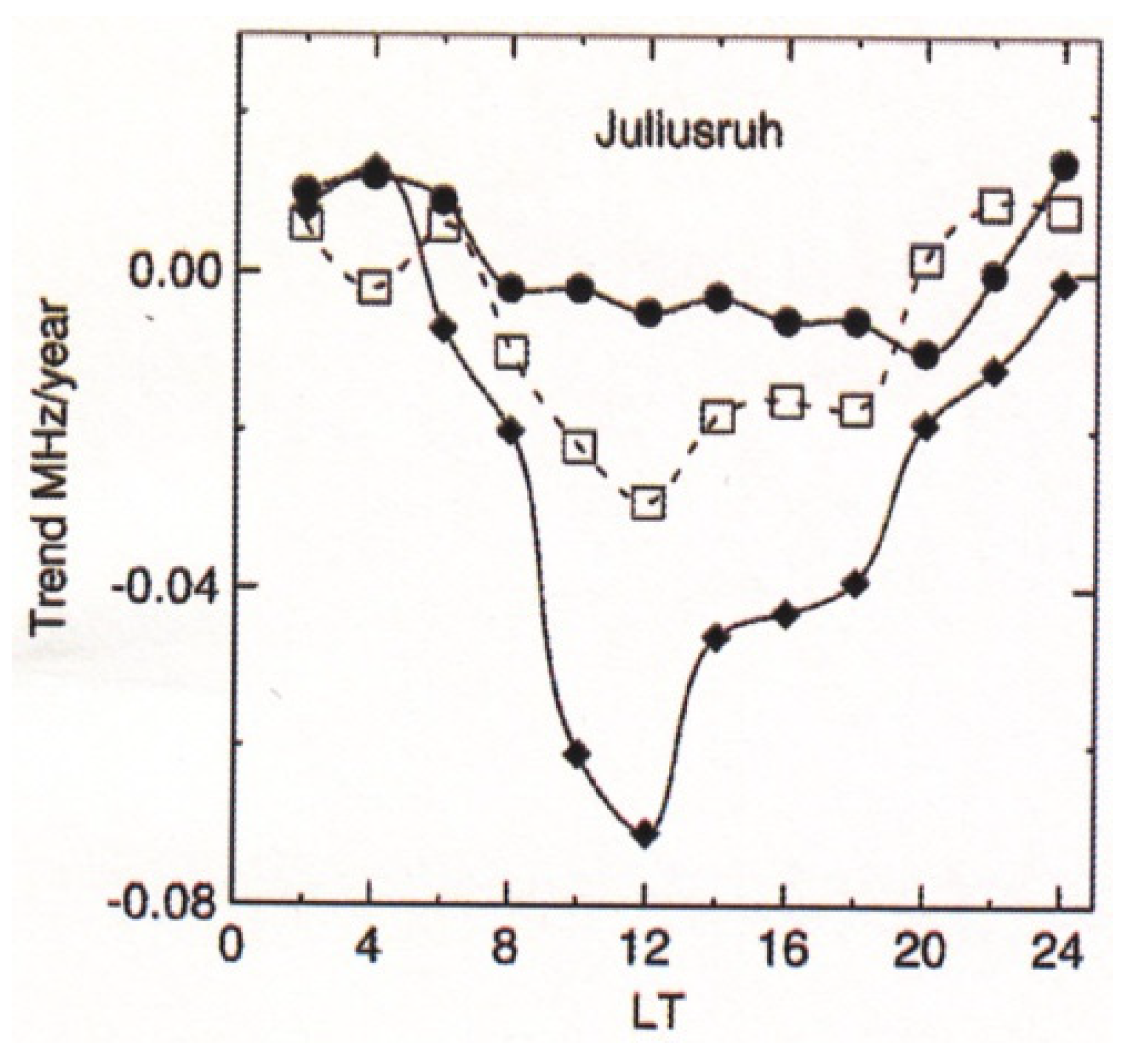
• Trends in foF2 are weak. They are mostly negative, but in some regions they are positive. Trends depend on the time of day and on the season; they are substantially stronger at midlatitudes in winter than in summer.
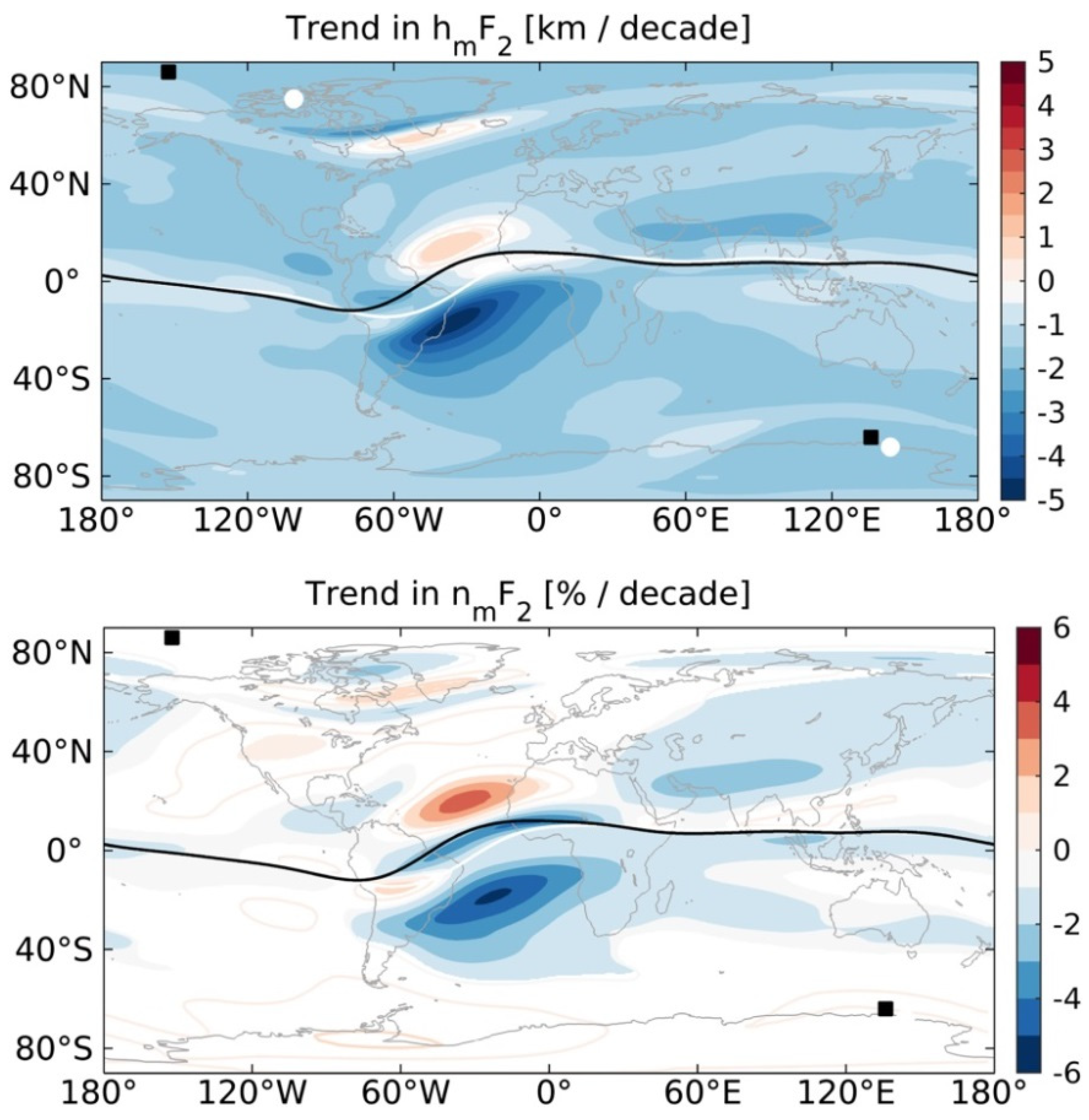
• There are more drivers of trends. Globally, the main driver of trends in foF2 is CO₂, but in some regions, the impact of secular changes in the Earth’s main magnetic field is stronger, the latter being negative in some areas and positive in others.
• There are various sources of uncertainty in calculating trends in foF2. Data homogeneity is one of them. The removal of the impact of much stronger solar cycles on foF2 data with optimum solar activity proxies is another. The application of different methods might result in somewhat different strengths in trends, e.g., those calculated by linear regression versus those based on the EEMD method.

The trends in foF2 have predominantly been studied at middle latitudes, partly at low latitudes, but very little at high latitudes. This should be improved in the future, together with model simulations of trends in foF2. Another task for the future is to study long-term trends in TEC more broadly due to their importance for GNSS signal utilization in positioning, among others. Until recently, such studies were limited by short data series.

References

- Alfonsi, L.; DeFranceschi, G.; Perrone, L. Long term trends of the critical frequency of the F2 layer at northern and southern high latitude regions. Phys. Chem. Earth 2002, 27, 607–612. [Google Scholar] [CrossRef]
- Bremer, J. Trends in the ionospheric E- and F-regions over Europe. Ann. Geophys. 1998, 16, 986–996. [Google Scholar] [CrossRef]
- Bremer, J. Long-term trends in the ionospheric E and F1 regions. Ann. Geophys. 2008, 26, 1189–1197. [Google Scholar] [CrossRef]
- Bremer, J.; Damboldt, T.; Mielich, J.; Suessmann, P. Comparing long-term trends in the ionospheric F2-region with two different methods. J. Atmos. Solar-Terr. Phys. 2012, 77, 174–185. [Google Scholar] [CrossRef]
- Chandra, H.; Vyas, G.D.; Sharma, S. Long-term changes in ionospheric parameters over Ahmedabad. Adv. Space Res. 1997, 20, 2161–2164. [Google Scholar] [CrossRef]
- Clilverd, M.A.; Ulich, T.; Jarvis, J.M. Residual solar cycle influence on trends in ionospheric F2-layer peak height. J. Geophys. Res. Space Phys. 2003, 108, 1450. [Google Scholar] [CrossRef]
- Cnossen, I. The importance of geomagnetic field changes versus rising CO2 levels for long-term change in the upper atmosphere. J. Space Weather Space Clim. 2014, 4, 18. [Google Scholar] [CrossRef]
- Cnossen, I.; Franzke, C. The role of the Sun in the long-term change in the F2-peak ionosphere: New insights from EEMD and numerical modeling. J. Geophys. Res. Space Phys. 2014, 119, 8610–8623. [Google Scholar] [CrossRef]
- Danilov, A.D. Long-term trends in F2-layer parameters and their relation to other trends. Adv. Space Res. 2005, 35, 1405–1410. [Google Scholar] [CrossRef]
- Danilov, A.D. Long-term trends in the relation between daytime and nighttime values of foF2. Ann. Geophys. 2008, 26, 1199–1206. [Google Scholar] [CrossRef][Green Version]
- Danilov, A.D. Seasonal and diurnal variations in foF2 trends. J. Geophys. Res. Space Phys. 2015, 120, 3868–3882. [Google Scholar] [CrossRef]
- Danilov, A.D. Behavior of F2 region parameters and solar activity indices in the 24th cycle. Geom. Aeron. 2021, 61, 102–110. [Google Scholar]
- Danilov, A.D.; Konstantinova, A.V. Relationship between foF2 trends and geographic and geomagnetic coordinates. Geom. Aeron. 2014, 54, 323–328. [Google Scholar] [CrossRef]
- Danilov, A.D.; Konstantinova, A.V. Long-term changes in the relation between foF2 and hmF2. Geom. Aeron. 2016, 56, 577–584. [Google Scholar] [CrossRef]
- Danilov, A.D.; Konstantinova, A.V. Trends in parameters of the F2 layer and the 24th solar activity cycle. Geom. Aeron. 2020, 60, 586–596. [Google Scholar] [CrossRef]
- Elias, A.G. Trends in the F2 ionospheric layer due to long-term variations in the Earth’s magnetic field. J. Atmos. Solar-Terr. Phys. 2009, 71, 1602–1609. [Google Scholar] [CrossRef]
- Laštovička, J. The best solar activity proxy for long-term ionospheric investigations. Adv. Space Res. 2021, 68, 2354–2360. [Google Scholar] [CrossRef]
- Laštovička, J.; Mikhailov, A.V.; Ulich, T.; Bremer, J.; Elias, A.G.; Ortiz de Adler, N.; Jara, V.; Abarca del Rio, R.; Foppiano, A.J.; Ovalle, E.; et al. Long-term trends in foF2: A comparison of various methods. J. Atmos. Solar-Terr. Phys. 2006, 68, 1854–1870. [Google Scholar] [CrossRef]
- Laštovička, J.; Yue, X.; Wan, W. Long-term trends in foF2: Their estimating and origin. Ann. Geophys. 2008, 26, 593–598. [Google Scholar] [CrossRef][Green Version]
- Mielich, J.; Bremer, J. Long-term trends in the ionospheric F2-region with different solar activity indices. Ann. Geophys. 2013, 31, 291–303. [Google Scholar] [CrossRef]
- Mikhailov, A.V. The geomagnetic control concept of the F2-layer parameter long-term trends. Phys. Chem. Earth 2002, 27, 595–606. [Google Scholar] [CrossRef]
- Perrone, L.; Mikhailov, A.V. Geomagnetic control of the midlatitude foF1 and foF2 long-term variations: Recent observations in Europe. J. Geophys. Res. Space Phys. 2016, 121, 7183–7192. [Google Scholar] [CrossRef]
- Qian, L.; Solomon, S.C.; Roble, R.G.; Kane, T.J. Model simulations of global change in the ionosphere. Geophys. Res. Lett. 2008, 35, L07811. [Google Scholar] [CrossRef]
- Qian, L.; Burns, A.G.; Solomon, S.C.; Roble, R.G. The effect of carbon dioxide cooling on trends in the F2-layer ionosphere. J. Atmos. Sol. Terr. Phys. 2009, 71, 1592–1601. [Google Scholar] [CrossRef]
- Ulich, T.; Turunen, E. Evidence for long-term cooling of the upper atmosphere in ionosonde data. Geophys. Res. Lett. 1997, 24, 1103–1106. [Google Scholar] [CrossRef]
- Upadhyay, H.O.; Mahajan, E.E. Atmospheric greenhouse effect and ionospheric trends. Geophys. Res. Lett. 1998, 25, 3375–3378. [Google Scholar] [CrossRef]
- Xu, Z.-W.; Wu, J.; Igarashi, K.; Kato, H.; Wu, Z.-S. Long-term ionospheric trends based on ground-based ionosonde observations at Kokubunji, Japan. J. Geophys. Res. 2004, 109, A09307. [Google Scholar] [CrossRef]
- Yue, X.; Wan, W.; Liu, L.; Ning, B.; Zhao, B. Applying artificial neural network to derive long-term foF2 trends in Asia/Pacific sector from ionosonde observations. J. Geophys. Res. 2006, 111, D22307. [Google Scholar] [CrossRef]
- Lastovicka, J.; Solomon, S.C.; Qian, L. Trends in the neural and ionized upper atmosphere. Space Sci. Rev. 2012, 168, 113–145. [Google Scholar] [CrossRef]
- Rezac, L.; Yue, J.; Yongxiao, J.; Russell, J.M., III; Garcia, R.; López-Puertas, M.; Mlynczak, M.G. On long-term SABER CO2 trends and effects due to nonuniform space and time sampling. J. Geophys. Res. Space Phys. 2018, 123, 7958–7967. [Google Scholar] [CrossRef]
- Cnossen, I. Analysis and attribution of climate change in the upper atmosphere from 1950 to 2015 simulated by WACCM-X. J. Geophys. Res. Space Phys. 2020, 125, e2020JA028623. [Google Scholar] [CrossRef]
- Jacobi, C.; Hoffmann, P.; Liu, R.Q.; Merzlyakov, E.G.; Portnyagin, Y.I.; Manson, A.H.; Meek, C.E. Long-term trends, their changes, and interannual variability of Northern Hemisphere midlatitude MLT winds. J. Atmos. Sol.-Terr. Phys. 2012, 75–76, 81–91. [Google Scholar] [CrossRef]
- Laštovička, J. A review of recent progress in trends in the upper atmosphere. J. Atmos. Sol.-Terr. Phys. 2017, 163, 2–13. [Google Scholar] [CrossRef]
- Danilov, A.D.; Konstantinova, A.V. Long-term variations of the parameters of the middle and upper atmosphere and ionosphere (review). Geom. Aeron. 2020, 60, 397–420. [Google Scholar] [CrossRef]
- Damboldt, T.; Suessmann, P. Consolidated Database of Worldwide Measured Monthly Medians of Ionospheric Characteristics foF2 and M(3000)FINAG Bulletin on Web, INAG-73, IAGA. 2012. Available online: https://www.ursi.org/files/CommissionWebsites/INAG/web-73/2012/damboldt_consolidated_database.pdf (accessed on 10 December 2021).
- Liu, H.; Tao, C.; Jin, H.; Abe, T. Geomagnetic activity effect on CO2-driven trend in the thermosphere and ionosphere: Ideal model experiments with GAIA. J. Geophys. Res. Space Phys. 2021, 126, e2020JA028607. [Google Scholar] [CrossRef]
- Yue, X.; Hu, L.; Wei, F.; Wan, W.; Ning, B. Ionospheric trend over Wuhan during 1947–2018: Comparison between simulation and observation. J. Geophys. Res. Space Phys. 2018, 123, 1396–1409. [Google Scholar] [CrossRef]
- Danilov, A.D.; Konstantinova, A.V. Trends in the critical frequency foF2 after 2009. Geom. Aeron. 2016, 56, 302–310. [Google Scholar] [CrossRef]
- Elias, A.G.; de Haro Barbas, B.F.; Shibasaki, K.; Souza, J.R. Effect of solar cycle 23 in foF2 trend estimation. Earth Plan. Space 2014, 66, 111. [Google Scholar] [CrossRef]
- Qian, L.; McInerney, J.M.; Solomon, S.S.; Liu, H.; Burns, A.G. Climate changes in the upper atmosphere: Contributions by the changing greenhouse gas concentrations and Earth’s magnetic field from the 1960s to 2010s. J. Geophys. Res. Space Phys. 2021, 126, e2020JA029067. [Google Scholar] [CrossRef]
- Laštovička, J. On the role of ozone in the long-term trends in the upper atmosphere-ionosphere system. Ann. Geophys. 2012, 30, 811–816. [Google Scholar] [CrossRef]
- Oliver, W.L.; Zhang, S.-R.; Goncharenko, L.P. Is thermospheric global cooling caused by gravity waves? J. Geophys. Res. Space Phys. 2013, 118, 3898–3908. [Google Scholar] [CrossRef]
- Oliver, W.L.; Holt, J.M.; Zhang, S.-R.; Goncharenko, L.P. Long-term trends in thermospheric neutral temperatures and density above Millstone Hill. J. Geophys. Res. Space Phys. 2014, 119, 7940–7946. [Google Scholar] [CrossRef]
- Laštovička, J. Comment on “Long-term trends in thermospheric neutral temperatures and density above Millstone Hill” by Oliver, W.L.; Holt, J.M.; Zhang, S.-R.; Goncharenko, L.P. J. Geophys. Res. Space Phys. 2015, 120, 2347–2349. [Google Scholar] [CrossRef]
- Laštovička, J.; Jelínek, Š. Problems in calculating long-term trends in the upper atmosphere. J. Atmos. Solar-Terr. Phys. 2019, 189, 80–86. [Google Scholar] [CrossRef]
- Pettitt, A.N. A non-parametric approach to the change point detection. Appl. Stat. 1979, 28, 126–135. [Google Scholar] [CrossRef]
- Alexandersson, H. A homogeneity test applied to precipitation data. J. Climatol. 1986, 6, 661–675. [Google Scholar] [CrossRef]
- Danilov, A.D.; Konstantinova, A.V. Behavior of the ionospheric F2 layer at the turn of the centuries. Critical frequency. Geom. Aeron. 2013, 53, 343–355. [Google Scholar] [CrossRef]
- Wu, Z.; Huang, N.E. Ensemble empirical mode decomposition: A noise-assisted data analysis method. Adv. Adapt. Data Anal. 2009, 1, 1–41. [Google Scholar] [CrossRef]
Publisher’s Note: MDPI stays neutral with regard to jurisdictional claims in published maps and institutional affiliations. |
© 2022 by the author. Licensee MDPI, Basel, Switzerland. This article is an open access article distributed under the terms and conditions of the Creative Commons Attribution (CC BY) license (https://creativecommons.org/licenses/by/4.0/).
Share and Cite
Laštovička, J. Long-Term Changes in Ionospheric Climate in Terms of foF2. Atmosphere 2022, 13, 110. https://doi.org/10.3390/atmos13010110
Laštovička J. Long-Term Changes in Ionospheric Climate in Terms of foF2. Atmosphere. 2022; 13(1):110. https://doi.org/10.3390/atmos13010110
Chicago/Turabian StyleLaštovička, Jan. 2022. "Long-Term Changes in Ionospheric Climate in Terms of foF2" Atmosphere 13, no. 1: 110. https://doi.org/10.3390/atmos13010110
APA StyleLaštovička, J. (2022). Long-Term Changes in Ionospheric Climate in Terms of foF2. Atmosphere, 13(1), 110. https://doi.org/10.3390/atmos13010110