Abstract
Dynamic numerical models of the atmosphere are the main tools used for weather and climate forecasting as well as climate projections. Thus, this work evaluated the systematic errors and areas with large uncertainties in precipitation over the South American continent (SAC) based on regional climate simulations with the weather research and forecasting (WRF) model. Ten simulations using different convective, radiation, and microphysical schemes, and an ensemble mean among them, were performed with a resolution of 50 km, covering the CORDEX-South America domain. First, the seasonal precipitation variability and its differences were discussed. Then, its annual cycle was investigated through nine sub-domains on the SAC (AMZN, AMZS, NEBN, NEBS, SE, SURU, CHAC, PEQU, and TOTL). The Taylor Diagrams were used to assess the sensitivity of the model to different parameterizations and its ability to reproduce the simulated precipitation patterns. The results showed that the WRF simulations were better than the ERA-interim (ERAI) reanalysis when compared to the TRMM, showing the added value of dynamic downscaling. For all sub-domains the best result was obtained with the ensemble compared to the satellite TRMM. The largest errors were observed in the SURU and CHAC regions, and with the greatest dispersion of members during the rainy season. On the other hand, the best results were found in the AMZS, NEBS, and TOTL regions.
1. Introduction
The South America continent (SAC) spreads over a large latitudinal extension, ranging from equatorial areas to mid-latitudes, and it is influenced by several weather and climate patterns. The South American climate and its variability are affected by remote, regional, and local forcings [1]. Understanding the mechanisms acting on these three scales of variability, in particular how they impact the hydrological cycle, is critical for medium range and seasonal precipitation forecasts. In turn, this is important for water resources management, hydro-power generation planning, and agricultural activities in SAC [2].
The use of dynamic numerical models is the basis of weather and climate forecasts around the world. The general circulation models (GCMs) have shown good ability at predicting and representing large-scale phenomena, also being employed for studies of future climate change scenarios [3]. However, the low spatial resolution hinders the accurate representation of mesoscale processes [3]. To improve the skill of global simulations, regional climate models (RCMs) with higher resolutions have been used for climate forecasting [4]. The higher accuracy of RCM simulations is partially due to better representation of the topography, coastlines, vegetation, and physical process parameterizations of meso and micro scales, which allow better representations of local influence factors on the climate of a particular region. For that reason, RCMs have become widely used to downscale low-resolution global climate simulations throughout different regions of the world. They provide a clear added value with respect to simulations with coarse resolution GCMs, particularly for variables, such as precipitation and near surface temperature [3,5,6].
COordinated Regional Climate Downscaling EXperiment (CORDEX)) [7] is a coordinated international effort whose goal is to improve the quality of downscaling in regional climate simulations with RCMs. Among other characteristics, CORDEX standardized reference areas for numerical studies. This strategy facilitates and adds quality to the intercomparison between simulation studies from different research groups. Within the several subgroups of CORDEX, there is the CORDEX-WRF component (http://www.meteo.unican.es/wiki/cordexwrf/CordexWrfHome, accessed on 18 August 2021) that concentrates on evaluating the weather research and forecasting model (WRF) [8]. In this way, the simulations carried out in this work are inserted in the CORDEX-WRF context, with special focus to the modeling of precipitation.
In recent decades, RCMs have been broadly used to produce climate change projections over the SAC region in an attempt to better capture regional and local feedback processes, e.g., the CLARIS project [9]. In particular, these studies have evaluated different RCMs to understand present day climate and future climate scenarios [10,11,12,13,14,15,16,17,18,19,20]. For a review of regional climate modeling studies over SAC, reference [1] summarized the main progress made since the early efforts at the beginning of the 2000s. They report that the earlier research aimed to test the ability of a diversity of RCMs (e.g., ETA, MM5, RegCM, among others) in reproducing basic aspects of seasonal climate, while from 2002 to 2007 the focus was on evaluating model performance and sensitivity. Since 2008 most of the efforts have been focused on the production of regional climate change scenarios. Reference [21] have made a compilation of the main studies using RCMs for South America.
In the current work, we assess the ability of the WRF model to reproduce the observed precipitation variability in SAC under the CORDEX-SOUTH AMERICA framework. Our focus is on the investigation of the optimal combination between radiation, convection, and microphysics schemes, and on the detection of systematic errors and areas with large uncertainties. The radiation parameterization schemes aim to estimate the total radiative flux and provide the shortwave heating and long wave cooling rates in the cloud layer. Radiation plays a significant role in the surface water–energy budget at the land surface. The total radiative flux is essential to calculate net radiation, sensible heat flux, and latent heat flux at the land surface. These fluxes also depend on the soil and vegetation types. Recently, the impact of radiation on these fluxes over the Amazon basin has been discussed by [22]. The microphysics scheme handles the phase changes of water, including cloud and precipitation processes. Finally, the convection parameterization schemes lead with the subgrid-scale representation of physical processes related to a wide range of cloud types, such as shallow, deep, and stratiform clouds at a horizontal resolution more major than cloud scale (<3 km). Convection is one of the key processes in atmospheric models, considering its important role in the atmosphere’s regional and global water and energy cycles by transporting heat, momentum, and moisture from the boundary layer to the free atmosphere. Moreover, convection is a significant driver of regional and global atmospheric circulations through the release of latent heat, as discussed by [23] on the South American summer upper-level circulation. In particular, in the tropics, where cumulus convection is extremely active, large amounts of precipitation and accompanied latent heat release play a key role in tropical atmospheric circulation and global energy balance [24]. As a consequence of this chain of mechanisms, different choices in radiation/convection/microphysics yield very different results in the simulated precipitation fields.
This study was conducted in a climate perspective (a 2-year simulation) instead of a weather forecast approach, which is the most frequent use of WRF. Despite this period being short compared to the usual climate timescale of 30-years, it does not prejudice the main goal of this study i.e., to find out which set of parameterizations is better suited to South America. In fact, longer simulations in the SAC using WRF are rare [25,26]. A similar study was made by [27], who applied the dynamical downscaling technique in the WRF model over the MED-CORDEX domain for a period of one year (2002), to investigate and validate the performance of different physics parameterizations. This study fills this gap and contributes toward the CORDEX effort over this region for subsequent climate modeling in future experiments. In addition, many users of the WRF model carry out research on different regions of the SAC and, therefore, our results can serve as a comparative reference.
2. Data and Methodology
2.1. Model Configuration and Numerical Experiments
Initial and lateral boundary conditions used to constrain the WRF model simulations are from the European Centre for Medium-Range Weather Forecasting (ECMWF) interim reanalysis (ERAI) [28]. The ERAI is the ECMWF global atmospheric reanalysis using the 4D-VAR data assimilation system, and it is a continuation of the previous ERA-40 atmospheric reanalysis dataset [28,29]. These data were available on a 0.75° × 0.75° grid from 1979 to 2019 at 6 h resolution for the 3D prognostic variables, which is a spatial resolution that agrees with our 50 km simulation. Despite the already available ERA-5 reanalysis (0.25° × 0.25°), its higher resolution is not suitable for driving 50-km regional model simulations, which several climate forecast centers in SAC still do, due to computer resource limitations.
Here, we use data from 2001 and 2002. The choice of these years had no special reason and they were chosen randomly from the dataset. In order to account for recent changes in land use (e.g., deforestation), updated datasets of land-surface albedo and greenness fraction at a high resolution were used instead of the standard WRF datasets (details in [30]).
Numerical simulations were conducted using the Advanced Research Weather Research and Forecasting model (WRF-ARW) version 3.9.1 [8]. The total simulated time is 16 months. It started at 00 UTC on 1 September, 2001, and finished on 21 UTC on 31 December 2002. The first four months of outputs were considered as the spin-up time, and were excluded from the final analysis. This is a more conservative approach than recommended by [4], and gives the model more time to equalize the surface hydrology with the external forcing, avoiding instabilities or drifts.
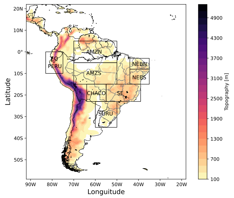
The simulations cover the CORDEX-South America domain (Figure 1) with a horizontal resolution of 50 km and 38 vertical levels with the top of the model at 50 hPa. The domain has 150 by 200 west-east and north-south grid points, respectively, in the Mercator projection.

Figure 1.
Domain and topography (m) used in the WRF simulations. The squares indicate the limits of sub-domains investigated. The abbreviations used in the map correspond to: Amazon basin NORTH (AMZN); Amazon basin SOUTH (AMZS); northeast of Brazil—NORTH (NEBN); northeast of Brazil—SOUTH (NEBS); southeast of Brazil (SE); south of Brazil and Uruguay (SURU); Chaco Region (CHAC), and Peru-Equator (PEQU).
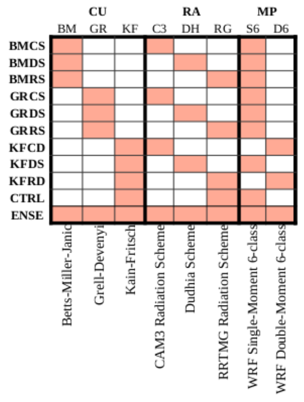
To examine the WRF model uncertainties in simulating the annual precipitation regime over South America, a sensitivity test was performed where we combined different physical parameterizations, as detailed in Figure 2. There are many different physics options in the WRF model for cumulus convection, turbulence, radiative transfer, gravity waves, microphysics, planetary boundary layer (PBL), land surface, etc. In the present study, we focus on cumulus parameterization (CU), radiation parameterization (RA) and microphysics (MP), while PBL (Mellor–Yamada–Janjic; MYJ) [31,32], surface layer (Monin–Obukhov Janjic; MOJ) [33,34] and land surface (Noah LSM) [35] schemes were kept fixed for all model configurations.

Figure 2.
Different model configurations adopted for each experiment for Cumulus parameterizations (CU, columns 1–3), radiation scheme (RA, columns 4–6) and microphysics (MP, columns 7–8). Abbreviations (BMCS, BMDS, BMRS, GRCS, GRDS, GRRS, KFCD, KFDS, KFRD, CTRL = control simulation, and ENSE = ensemble) are described in text.
A total of 10 simulations were run, corresponding to the 10 different model configurations (see Figure 2). The ensemble mean was also evaluated. The ensemble mean experiment was generated from the mean of ten individual members. Three convection schemes were used, namely the Kain–Fritsch (KF) [36,37], Grell–Devenyi (GR) [38], and Betts–Miller–Janjic (BM) [39]. Three radiation schemes were used as well, the newer version of the rapid radiative transfer model (RG) [40], Dudhia scheme (DH) [41], and CAM scheme (C3) [42]. As for the microphysics, we evaluated the WRF single-moment six-class scheme (S6) [43] and WRF double-moment six-class scheme (D6) [44]. We considered the control simulation (CTRL) as the combination of KF cumulus scheme, RG radiation scheme, and S6 scheme for the cloud microphysics, which is the mostly employed model setup in operational forecasting in the SAC domain. For each model configuration, there is one or more model configurations that differ in just one of the parameterizations, allowing to evaluate the effect of changing each one in isolation.
2.2. Model Evaluation
The evaluation of the different model configurations was conducted in two ways. First, Tropical Rainfall Measuring Mission (TRMM) [45] version 3B42 V7 data were used as the “observational truth”. TRMM has been widely used over South America [46,47,48], and recent studies [49] have shown a satisfactory agreement with ground observations by meteorological stations.
The evaluation of monthly precipitation variability and model systematic errors were performed for each of the CORDEX sub-domains shown in Figure 1. These are named as AMZN (North Amazon, 5° S–5° N; 70° W–50° W), AMZS (South Amazon, 15° S–5° S; 70° W–50° W), NEBN (north–northeast Brazil, 8° S–3° S; 44° W–35° W), NEBS (south–northeast Brazil, 15° S–8° S; 44° W–35° W), PEQU (Peru-Equator, 10° S–0°; 83° W–75° W), CHAC (Chaco region, 23° S–15° S; 64° W–55° W), SUDE (southeast Brazil, 23° S–15° S; 55° W–39° W) and SURU (south Brazil and Uruguay, 35° S–23° S; 60° W–50° W). The TOTL region is the area-weighted average of all sub-domains.
The simulated monthly average precipitation was assessed using Taylor diagrams [50]. These diagrams summarize the degree of similarity between each WRF experiment and the reference data with respect to the standard deviation (SD), root-mean-square error (RMSE), and Pearson correlation coefficient. These diagrams are especially useful in assessing multiple aspects of complex models or in gauging the relative skills of many different models simultaneously. In addition to Taylor diagrams, we used box-plot diagrams to evaluate whether errors were random or systematic in the annual cycle. For some of the analysis, we grouped the sub-domains in three representative regions: tropical (AMZN, AMZS, NEBN, NEBS, and PEQU; from 15° S to 5° N), subtropical (CHAC and SUDE; from 23° S to 15° S) and extratropical (SURU; from 35° S to 23° S).
3. Results
3.1. Seasonal Analysis
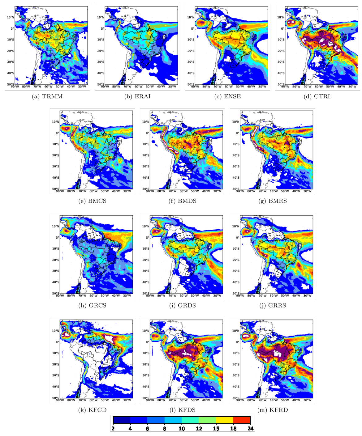
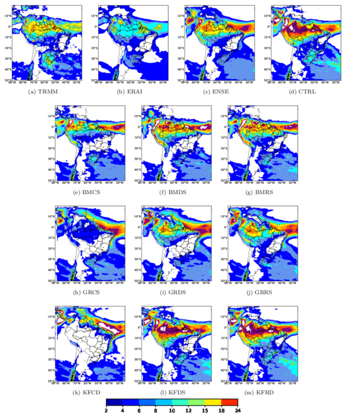
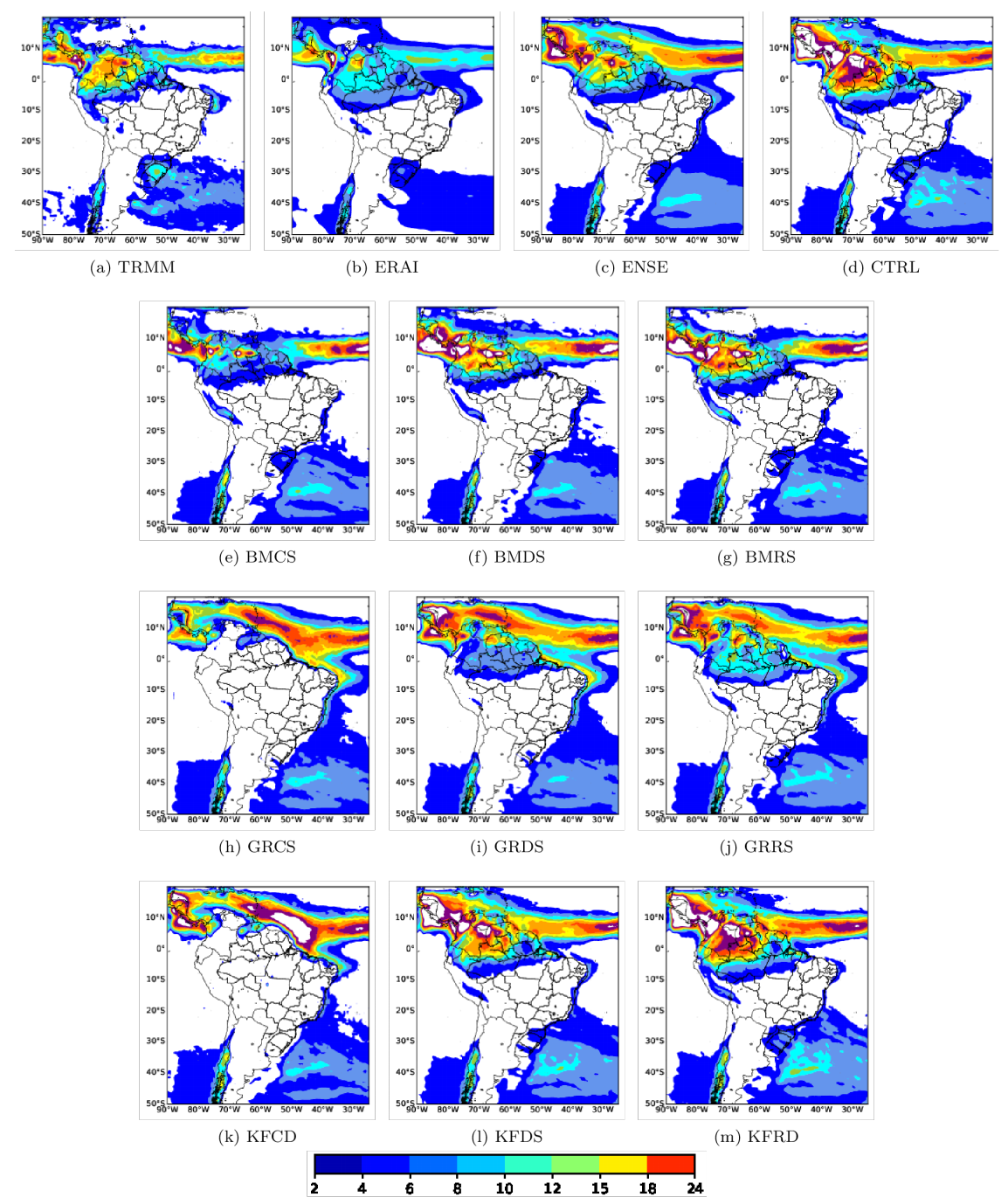
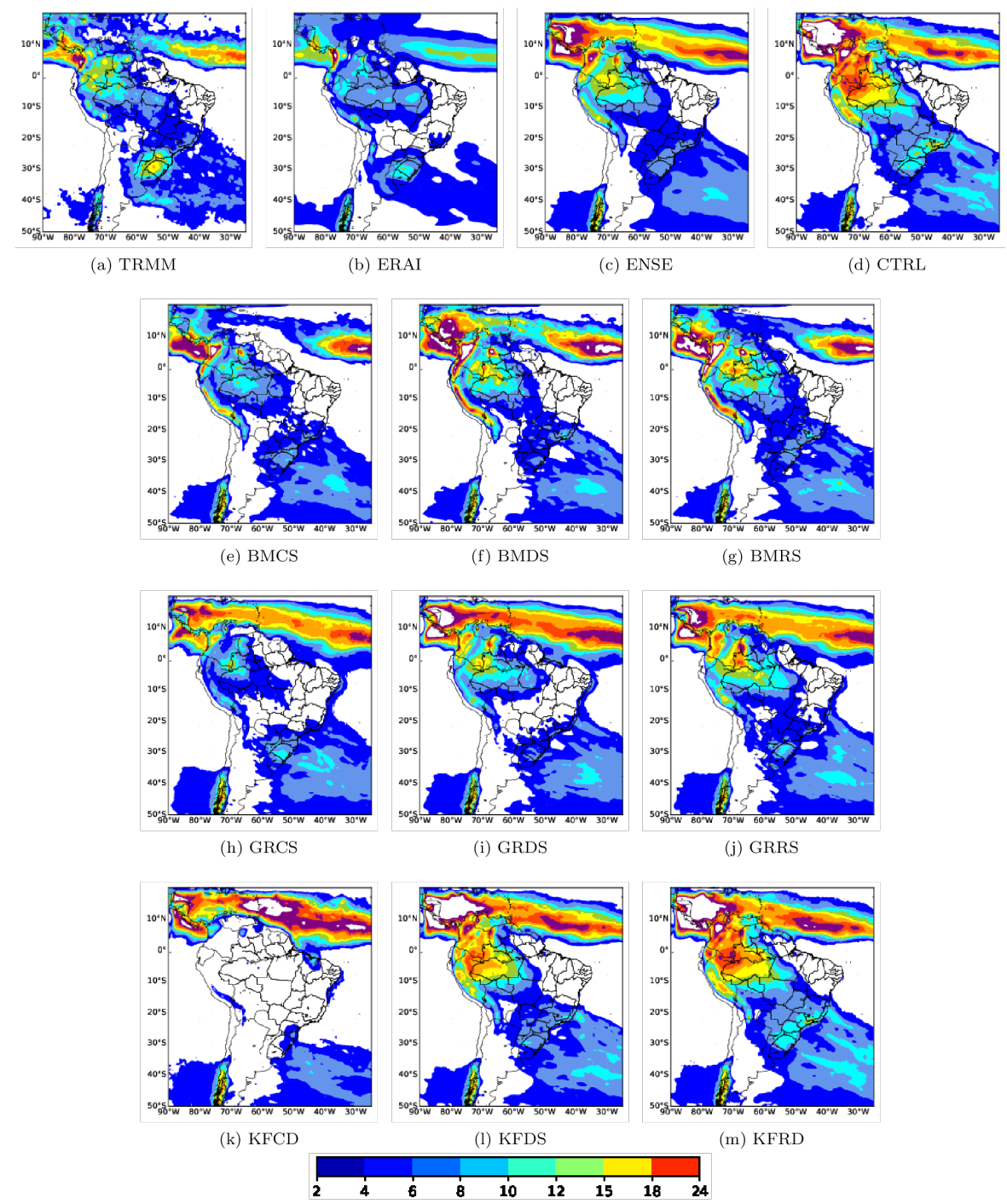
Figure 3, Figure 4, Figure 5 and Figure 6 show the average daily precipitation field for the DJF/MAM/JJA/SON quarters, respectively. The first line of plots contains the observation reference data by TRMM; the original input data to the simulations, ERAI reanalysis; the mean of ten individual members (ENSE = ensemble); and the control simulation (CTRL). These four plots are hereafter referred to as “reference cases”, and the individual simulation in the three remaining lines as “individual members”, or simply “members”.
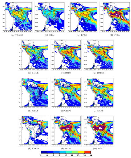
Figure 3.
Precipitation fields for December–January–February (in mm/day). The first line of plots is for TRMM, ERAI, ENSEMBLE, and control simulations (CTRL). The next lines represent one of each member, as described in Figure 2.

Figure 4.
As in Figure 3, but for March–April–May quarter.
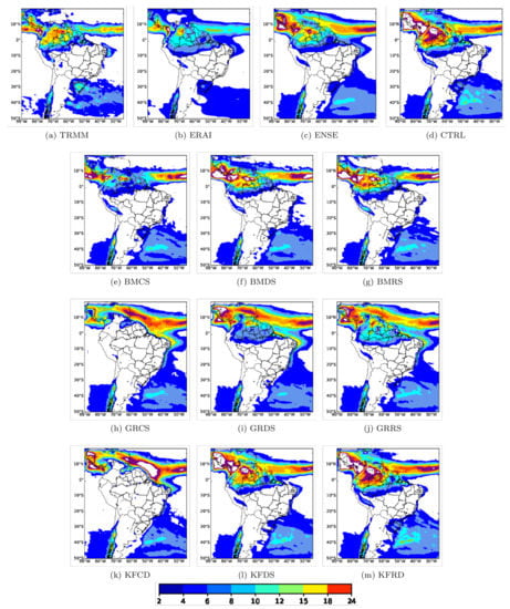
Figure 5.
As in Figure 3, but for June-July-August quarter.

Figure 6.
As in Figure 3, but for September–October–November quarter.
In SAC, most of the precipitation volume falls on DJF, which is shown in Figure 3. This wet period, in some specific areas, extends to March. This is the case for the majority of the Amazon basin, southeast and northeast Brazil, Peru, and Central South America. Northern portions of Amazonia, which is partially in the northern hemisphere, have their wet season shifted forward to April and May. On the other hand, the winter months of JJA (Figure 5) are the driest in the majority of the continent (except for the north hemisphere portion of SAC, subject to inter-tropical convergence zone (ITCZ) influence, as can be seen in Figure 3).
With respect to the wet trimester DJF (Figure 3), it is possible to see that TRMM and the reference cases agree, with respect to the spatial pattern of precipitation, but clearly disagree with respect to their precipitation volumes. While CTRL overestimates the observed values, ERAI underestimates it, and the ENSE of simulations is closer to TRMM than both CTRL and ERAI. This improvement of ENSE is an important result, and demonstrates that an ensemble based on physical parameterizations, plus the finer resolution was capable of providing more accurate results than the reanalysis fields from ERAI. Looking onto specific members (lines 2–4 of plots), it is possible to see that the general spatial pattern of precipitation is correct for most of them, except for GRCS and KFCD that largely underestimated rain in the center of SAC, and KFDS/KFRS, whose results went in the opposite direction i.e., largely overestimated precipitation. The results for the Kain–Fritsch parameterization are surprising, and they suggest that it is the combination of radiation and microphysics that determines precipitation fields when KF is the chosen cumulus parameterization. Given that microphysics at the resolution of 50 km is a weak forcing, and that convective storms dominate the scene in the wet season in SAC, it seems that the radiation choice is the critical parameter when KF is employed.
The following quarter MMA is shown in Figure 4. For the rainy equatorial latitudes, the same bias of TRMM, ERAI, ENSE, and CTRL was observed. Important differences can be seen in rain volume in South of Brazil, Uruguay, and Argentina. For these regions, the CTRL setting seems to better represent rain, while ENSE and ERAI underestimate precipitation. Dry regions (eastern portion of Brazil, central Argentina) were kept dry for the totality of members, and all simulations were capable to produce rain in the southern portion of Chile with little difference among them.
The dry season in SAC, the quarter JJA, was well reproduced in a broad sense by all members, CTRL, ENSE, and ERAI (Figure 5. Some differences remain for the SURU region, where an underestimation of precipitation was observed in all cases (when directly compared to TRMM).
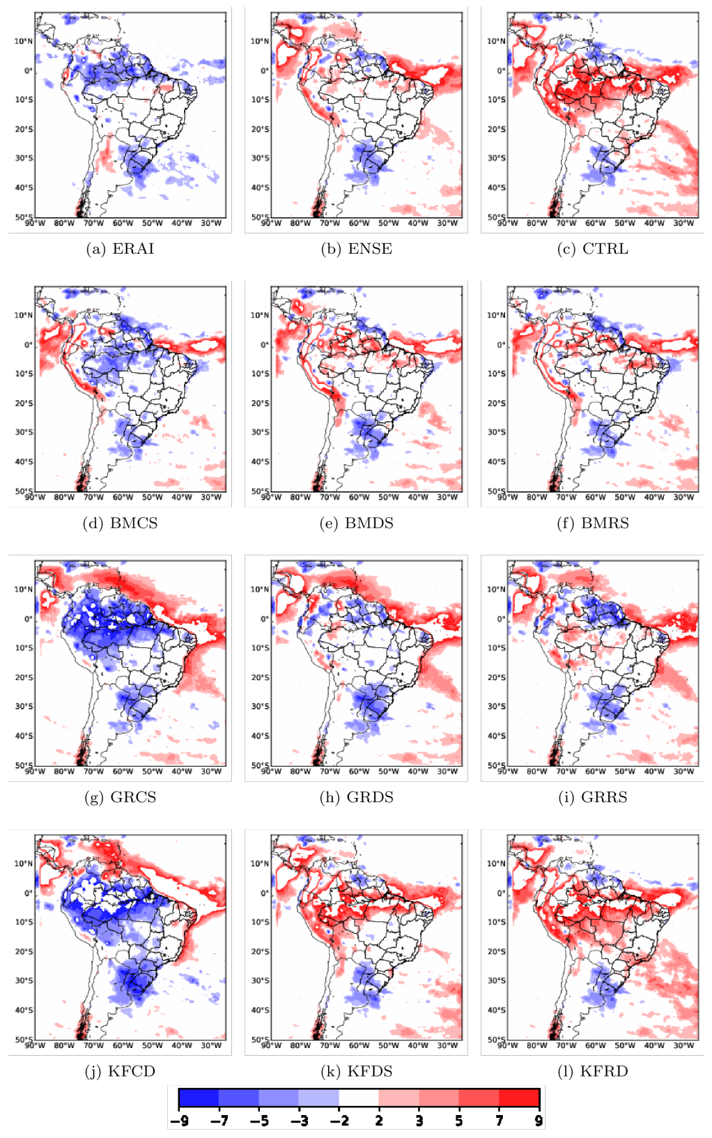
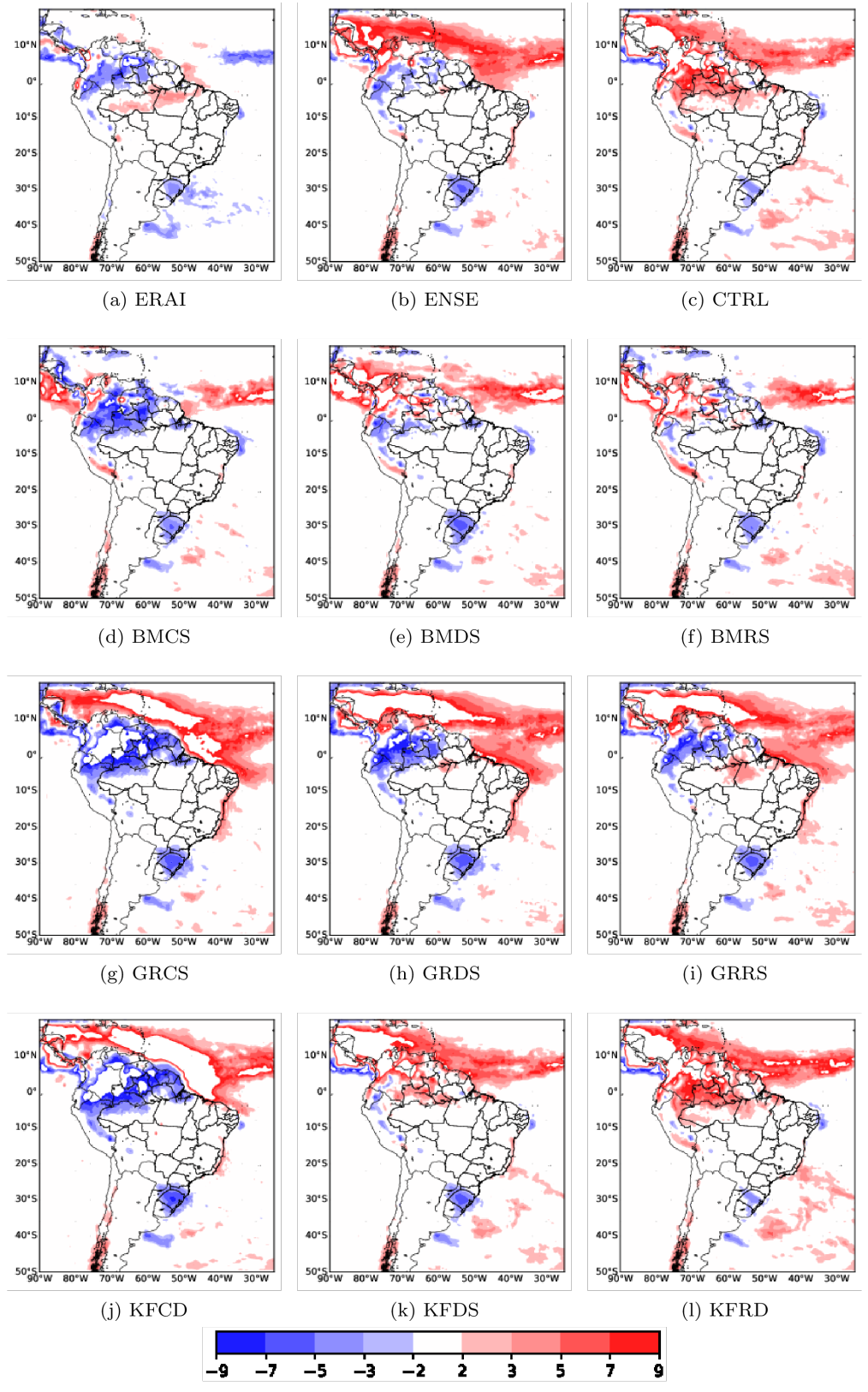
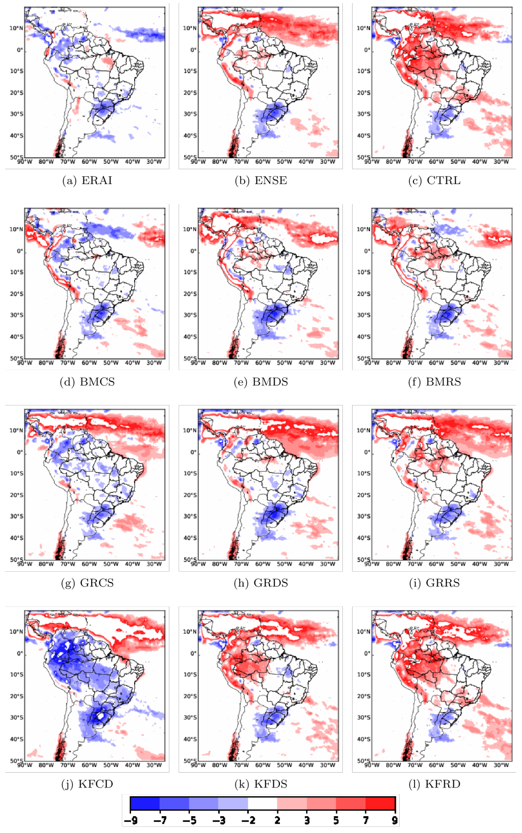
The quarter SON is the dry-to-wet transition in most of the SAC. As can be seen in Figure 6, important spatial differences were obtained for the reference cases ENSE, CTRL, and ERAI, as well for individual members. These differences (anomaly) also comprise the precipitation volumes. These differences can be better discussed by the analysis of the anomalies between reference cases and individual members to the observational reference of TRMM data. These anomalies are shown in Figure 7, Figure 8, Figure 9 and Figure 10.
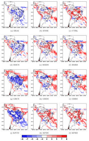
Figure 7.
Deviations of simulated precipitation fields to the observational reference (TRMM) for the December–January–February quarter, in mm/day.
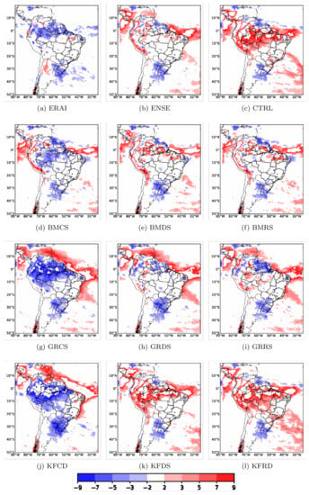
Figure 8.
As in Figure 7, but for March–April–May quarter.
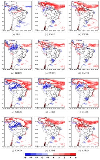
Figure 9.
As in Figure 7, but for June–July–August quarter.
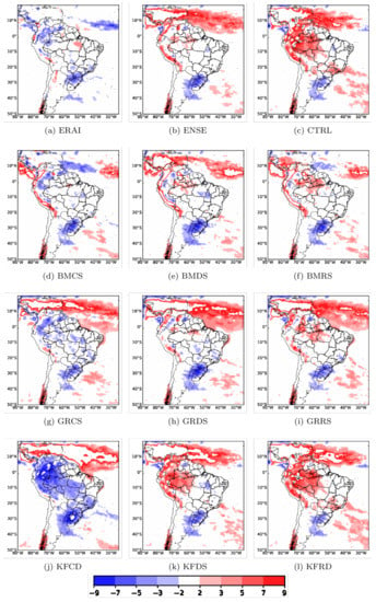
Figure 10.
As in Figure 7, but for September–October–November quarter.
A common feature for all months, for both reference and member cases, is an underestimated precipitation in the SURU area. Apparently, there is an intrinsic difficulty to correct simulate precipitation in this region, which is partly due to its difficulty in simulating cold fronts, and which seems to be a known phenomenon already observed in previous studies [51,52,53,54].
With respect to the anomalies in DJF, one can see in Figure 7 that ERAI mostly underestimate precipitation in the SAC while ENSE anomalies are more evenly distributed throughout the continent. CTRL simulations presented more positive anomalies inside the continental area, except for a few areas in the extreme northeast coast of Brazil and north of Argentina. For individual members, all on them in the left column underestimated precipitation over continental area. In common, they employed the C3 radiation scheme. This spatially broad negative anomaly was observed for all convection parameterizations, which is a clear demonstration that C3 induces a negative bias during wet season. Looking into the other six members, a general result is the already mentioned underestimation in SURU area.
In the fall (MAM, Figure 8), among the reference cases, ENSE presented the best result with a smooth distribution of anomalies though the three reference cases except the underestimation in the SURU area. In the Equator region, CTRL overestimated precipitation in the south of the Amazon River, while ERAI showed the opposite sign but in the north side of the same Amazon River course. With respect to individual members, those using the C3 scheme (left column) still underestimate precipitation. Member with KF cumulus parameterization greatly differed again, showing the strong dependence on the radiation scheme.
For JJA (the driest quarter, Figure 9), there is a good agreement for the continental area. In fact, most positive anomalies are over the ocean, following the climatological position of ITCZ. The few areas with anomalies in the continent are over the west and central portions of Amazonia and SURU domain, with ENSE showing the best results.
Finally, in the dry-to-wet transition quarter of SON (Figure 10), it is noteworthy the ERAI and ENSE low deviations in continental areas (except for the underestimation in SURU). However, ENSE produced significant positive deviations in the north of the Atlantic ocean (ITCZ area). Either way, both got results far superior to the CTRL experiment, which resulted in significant portions of the Amazon basin with negative deviations. Among the individual members, the KFCD experiment presented a large area with negative deviation in the continental portion of the domain. Interestingly, this pattern was not followed by the other C3 schemes (on the left column—as observed in the DJF quarter; Figure 7). A possible explanation for this behavior is that the convection schemes in BMCS and GRCS were partially able to counterpart the bias induced by C3 in SON, but not in DJF. Further investigation is necessary to corroborate (or not) this hypothesis.
3.2. Evaluation of Sub-Domain Annual Cycle
In this section, the general behavior of the simulation ensemble performed in this study is evaluated with the observational results of the TRMM satellite and the reanalysis for each subdomain. This part of the analysis aims to verify the level of agreement and coherence between these datasets in a broader approach before discriminating by a numerical experiment.
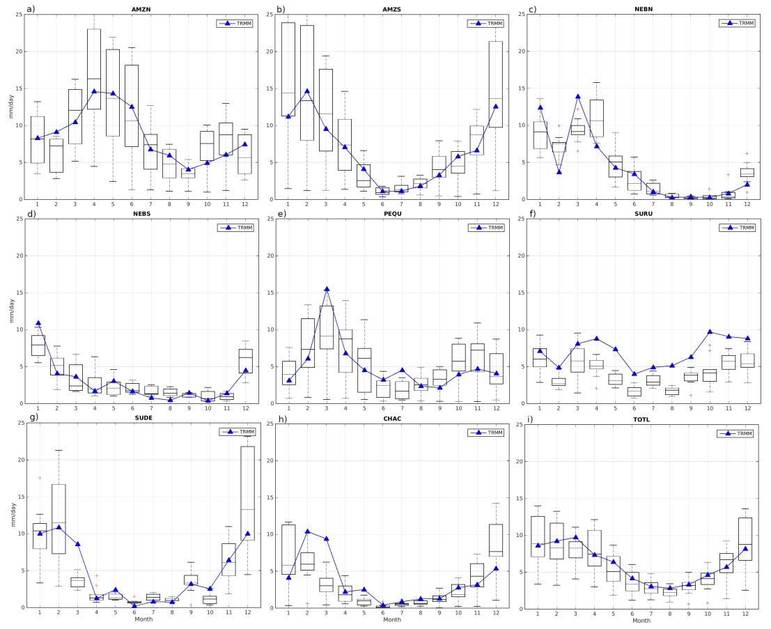
Figure 11 shows for each subdomain the time series of simulated precipitation (boxplots based on the 10 members) and the corresponding TRMM satellite monthly totals.
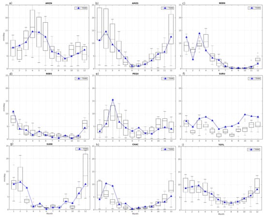
Figure 11.
Direct comparison of the annual cycle of simulated ensembles and observations for the eight areas investigated in this study [(a) AMZN, (b) AMZS, (c) NEBN, (d) NEBS, (e) PEQU, (f) SURU, (g) SUDE, (h) CHAC], plus the average over all areas [(i) TOTL]. Box plots represent the statistical spread of monthly precipitation for all nine members + CTRL. Here, they follow the standard format of box plots, i.e., boxes represent quartiles, and whiskers are of 1.5 interquartile range, far from the box limits. Red crosses represent outliers outside this range. The blue line corresponds to TRMM data.
3.2.1. Amazon Basin (AMZN + AMZS)
For both sub-domains corresponding to the Amazon basin (Figure 11a,b) there is a good general agreement between simulations and TRMM, though a few differences are noteworthy to highlight. At the AMZN subdomain, during the rainy months (January–April), there is a negative anomaly for February that is compensated in April, with a positive anomaly of similar magnitude. This difference is not observed for AMZS, except for a small difference in January. In spite of this small differences, ENSE x TRMM has excellent agreement in the annual cycle.
3.2.2. Northeast of Brazil (NEBN + NEBS)
In general, ENSE and TRMM agree very well on the annual precipitation cycle in both sub-domains that represent the northeast region (NEBN and NEBS). The biggest discrepancy was for the NEBN region in the months of March/April, which is more influenced by ITCZ when compared to the rest of the northeast region as a whole (especially in the coastal region).
The northeast of Brazil is influenced by several meteorological systems, whose intensity varies according to the portion under analysis: ITCZ, cold/stationary fronts, land and sea breeze [55], and easterly wave disturbances [56,57]. The relative influence of each system varies significantly within the NEBN subdomain itself. Thus, the results of this work show that, on average, the models do not capture this relative modulation of meteorological components in a satisfactory way especially for the wettest months (March/April), and more detailed studies are necessary to understand the reason. Here, we hypothesize that the dispersion between ENSE/TRMM is probably due to spatial differences within the NEBN and NEBS boxes, such as between the coastal region and the semi-arid center. Another aspect is that, for March, the interquartile range (IQR) of the ENSE/NEBN is very low, which shows that the choice of parameterizations is indifferent with respect to making the model agree with the TRMM observation. Differently, IQR for April is significantly larger than March, which shows the difficulty in adjusting the real precipitation. Again, the likely explanation is a possible inhomogeneity in precipitation field within the NEBN domain, which could generate bias in the TRMM observational mean. Anyway, in an integrated bimonthly perspective (March/April), the ENSE approximately hits the total rainfall. A better accuracy in this type of forecast would be of great value, for example, for local agriculture, given the low total rainfall of the NE region as a whole.
3.2.3. South of Brazil and Uruguay (SURU)
As already discussed in Figure 3, Figure 4, Figure 5, Figure 6, Figure 7, Figure 8, Figure 9 and Figure 10 (seasonal maps), both reference cases and individual members underestimated the precipitation observed by the TRMM satellite. Figure 11f shows that the monthly rainfall curve is systematically above all boxplots. In fact, most of the current operational regional and global atmospheric models used in numerical weather and climate prediction and CMIP models still show serious deficiencies in simulating the precipitation during the wet season over South America, and the La Plata Basin. In general, models tend to underestimate rainfall over these regions as shown in previous studies [51,52,53,54]. In fact, it is a region where models perform with low skill, mostly because the success of the simulation depends on a precise determination of a low level jet, cold fronts passage, and the generation of mesoscale convective systems (quite common in this region). Even small changes in the position of these meteorological systems induce huge changes in the precipitation fields. This is the case with our simulations in the SURU sub-domain, which is under the influence of all these mechanisms.
However, in spite of the systematic errors, one can see that the annual cycle is captured in a general way, with annual minimums in the winter months (JJA), and maximums in March/April and November/December.
3.2.4. Peru/Equator (PEQU), Chaco (CHAC), and Southeast of Brazil (SUDE)
For this sub-domain, the annual cycle was captured in an excellent way, in spite of some dispersion of members in the rainy season. For most of the year, the observed data are very close to the medians. At CHAC, simulations caused an earlier onset of the rainy season, resulting in maximum precipitation in January while observational maxima was in February. It is noteworthy to mention that the agreement in the PEQU is surprisingly good, especially considering that this is an area of rugged relief due to the Andes, and a 50 × 50 km resolution usually fails to capture the influence of topography on the intense orographic precipitation associated.
3.2.5. Average over All Domains (TOTL)
The last plot shows the area-weighted daily average precipitation for all simulated domains, and the corresponding TRMM observations. The agreement between simulations and observations is excellent, and the correct reproduction of the annual cycle is remarkable, except for March, when simulations underestimated the actual precipitation. Another point to highlight is the very low variability of simulations during the dry months. In fact, the interquartile Range for July–October is very low, which means that models not only agree with observations, but they also agree with each other.
4. Best Sub-Domain Settings—Taylor Diagrams Analysis
To assess the sensitivity of the model to different parameterizations and its ability to reproduce the simulated precipitation patterns, an analysis was performed using Taylor diagrams. These kinds of diagrams synthesize, in a single plot, the relevant parameters for choosing the best model from a statistical point of view. Thus, it was investigated how well each member (i.e., its precipitation field) agrees with the TRMM observations in terms of root mean square error (RMSE), correlation coefficient (R), and standard deviation (STD). Note that the model’s ability to simulate the reference precipitation, as well as the impact of changing the parameterization schemes, resulted in different behaviors for each sub-domain.
4.1. Amazonia
In the AMZN region (Figure 12a), the ENSE obtained the most consistent result with respect to the reference data, with R = 0.91, RMSE = 0.4, and the same STD as the TRMM data. However, as the computational costs to generate a nine-member ENSE is prohibitive in most operational centers in SAC, we can attribute the BMRS experiment as the best alternative. The GRDS simulation obtained the same STD as the reference data, but with lower R and higher RMSE. With respect to the cumulus parameterization, BM presented the best and KF the worst result. Regarding the radiation scheme, a negative impact is evident when using option C3.
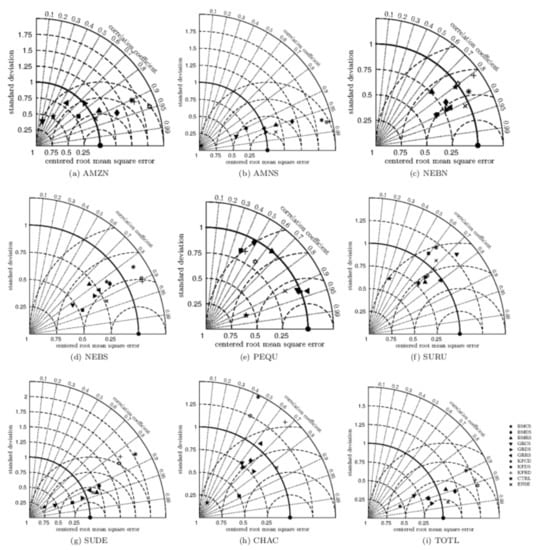
Figure 12.
Taylor diagrams for area-averaged monthly precipitation in regions (a) AMZN, (b) AMZS, (c) NEBN, (d) NEBS, (e) PEQU, (f) SURU, (g) SUDE, (h) CHAC, and (i) TOTL shown in Figure 1. The reference (TRMM) data are shown by the closed circle along the horizontal axis. The individual experiments are shown by different forms.
Figure 12b shows that in the AMZS region, the model obtained more consistent agreement with TRMM data than observed in the AMZN region. We attribute this difference to the fact that the precipitation AMZN is modulated by the ITCZ [58], whose position in March 2002 was further north of its climatological position, and in April, further south (data not shown), which may have resulted in the model’s difficulties in predicting such anomalies. In the AMZS region, the GR cumulus parameterization obtained the best results, unlike AMZN, where the GRDS and GRRS simulations presented the same STD as the TRMM. However, GRDS had slightly higher R and lower RMSE. The cumulus KF parameterization showed the worst results, with high RMSE and STD.
In both regions, the use of the D6 microphysics had a negative impact with the cumulus KF parameterization, with a strong reduction in the correlation with the reference data. The KF scheme uses low-level vertical movements as a trigger function and the removal of convective potential energy available as a closure. In fact, according to [59], in the Amazon region, the available convective potential energy (CAPE) varies with the intensity of convection, but does not explain convection variations, suggesting that a convective parameterization based on CAPE does not capture the observed behavior.
4.2. Northeast of Brazil
In the NEBN region (Figure 12c), the model’s sensitivity to parameterization changes is small when compared to the AMZN and AMZS regions. The GR and BM parameterizations obtained very similar results, except for the BMRS experiment, with the worst performance for this region. GR had higher correlations compared to the TRMM and lower RMSE values, with the GRRS option being slightly more consistent. In general, the model was not very sensitive to changes in convective parameterization in this region, except when using the RRTMG scheme, which had a negative impact when combined with the BM and KF schemes. The best performance was obtained with ENSE, the same occurring in the NEBS region (Figure 12d). In this region, the KFDS and KFRD configurations presented results slightly more consistent with what was observed.
4.3. Andes
The Peru-Ecuador region (Figure 12e) presents a strong sensitivity of the model to the choice of parameterization schemes used. It is evident that the Grell parameterization obtained the best results, regardless of the radiation scheme, which in this case was insignificant. It is noteworthy that the GRDS and GRRS experiments had the same STD as the reference data, but GRDS was slightly superior and had lower RMSE. The BM and KF experiments showed low correlations with the TRMM (except the CTRL experiment), and high RMSE values. Again, ENSE obtained a result consistent with the reference data.
4.4. South of Brazilian and Uruguay
In the SURU region (Figure 12f), the GRRS experiment (KFCD) presented the result more consistent with what was observed. Similar to what happened in the NEBN region, this region is not very sensitive to changes in the parameterization schemes. A highlight of this region is that the use of the C3 radiation scheme had a negative impact, regardless of the cumulus parameterization.
4.5. Southeast Brazil
The best result for the SUDE region (Figure 12g) was obtained with the GRDS option, while the cumulus KF parameterization scheme presented the worst results, regardless of the radiation scheme used. This result is in agreement with the study by [60], who evaluated the ability of the MM5 model to simulate intraseasonal variability during the warm season over South America through sensitivity experiments, and their results showed that Grell’s cumulus scheme was most suitable for subtropical latitudes.
4.6. Chaco
In the Chaco region (CHAC), as in other sub-domains, the ENSE option obtained the most consistent result compared to TRMM (Figure 12h). Individually, the BMCS experiment showed the highest correlation with the reference data and the lowest RMSE, being the most recommended. Regarding the experiments with the GR cumulus scheme, these showed low sensitivity when the radiation scheme was changed.
4.7. All Sub-Domains (TOTL)
Considering the total area (Figure 12i) the most consistent results, compared to TRMM are the ENSE and the GRDS experiment, while the largest errors are from the experiments using KF, as expected, in view of the results presented and discussed in the individual sub-domains.
The microphysics scheme was changed only using KF. It was possible to observe that the impact is negative when using option D6 in the PEQU and CHAC regions, and slightly less significant in the NEBS, SURU, SUDE, and TOTL regions. In other areas, there was no impact.
5. Summary and Conclusions
This study evaluated the systematic errors and areas with large uncertainties in a simulated precipitation over the South American continent. Different convective, radiation, and microphysical schemes of the WRF model were tested. The analyses through Taylor diagrams showed that, in all sub-domains, the ensemble of all experiments was the best option, with results consistent with those from the satellite data obtained from TRMM. The results also showed that the WRF simulations were better than those of the ERAI reanalysis, which was used as initial and boundary conditions for the WRF model, showing the added value of dynamic downscaling.
Regarding the choice of the convective parameterization scheme, the GR parameterization was the best option in most areas (AMZS, NEBN, PEQU, SURU, and SUDE), and satisfactory in other areas. On the other hand, the worst results were obtained with KF, with greater errors and lower correlations. In terms of radiative parameterization scheme, the impact in the precipitation distribution and seasonality was less than the convective parameterization, as expected. The DH and RG options performed better, as well as the S6 microphysical scheme. The GRDS configuration turned out to be the best configuration for the total domain and KFRD the worst.
The largest errors were in the SURU and CHAC regions, and in some experiments in the PEQU region. The evaluation of the annual cycle showed that the model was able to reproduce the variations in precipitation in most regions, highlighting the SURU region, which is a region in which precipitation occurs throughout the year. This region stood out for also presenting greater systematic discrepancies. In addition to these facts, it was also noted that the greatest dispersion of members was concentrated in the rainy periods.
This study comes to fill this gap and to contribute to the CORDEX effort over the South American region for future climate model experiments and downscaling efforts. In addition, many users of the WRF model carry out research on different regions of the SAC and, therefore, our results can serve as a comparative reference. The important conclusion that can be drawn from this work is that WRF simulations accurately reproduces features at several time scales over the SAC and, additionally, it provides information at spatial scales not resolved by GCMs that can be extremely useful in the studies of climate change scenarios.
As a future activity, we intend to apply the Brazilian Global Atmospheric Model (BAM), which is the atmospheric module of the Brazilian earth system model (BESM), as initial and boundary conditions on the WRF model, aiming to predict the sub-seasonal to seasonal and climate variability on specific regions of South America and Brazil. Moreover, based on the new implementation of aerosol-cloud microphysical interactions and cloud processing of aerosols in BAM, we will investigate the effects of aerosols on seasonal rainfall in South America at the regional scale.
Author Contributions
Conceptualization and design of the simulations, H.B.G. (Helber Barros Gomes), M.C.L.d.S., H.d.M.J.B. and T.M.P.J.; calculations, H.B.G. (Helber Barros Gomes), M.C.L.d.S. and T.M.P.J.; analysis, H.B.G. (Helber Barros Gomes), M.C.L.d.S., H.d.M.J.B, T.A., H.B., H.B.G. (Heliofábio Barros Gomes), F.D.d.S.S., R.L.C., S.N.F., D.L.H. and T.M.P.J.; writing—original draft preparation, H.B.G. (Helber Barros Gomes), M.C.L.d.S., H.d.M.J.B., S.N.F. and T.M.P.J.; final review, H.B.G. (Helber Barros Gomes), M.C.L.d.S., H.d.M.J.B., T.A., H.B., H.B.G. (Heliofábio Barros Gomes), F.D.d.S.S., R.L.C., S.N.F., D.L.H. and T.M.P.J. All authors have read and agreed to the published version of the manuscript.
Funding
This work was partially funded by the following project of the Coordination for the Improvement of Higher Education Personnel (CAPES, acronym in Portuguese), through grant CAPES/Modelagem 88881.148662/2017-01.
Institutional Review Board Statement
Not applicable.
Informed Consent Statement
Not applicable.
Data Availability Statement
The datasets used in this study as initial and boundary conditions for the WRF model simulations and validation were obtained from the European Centre for Medium-Range Weather Forecasting (ECMWF) and Tropical Rainfall Measuring Mission (TRMM) version 3B42 V7, respectively. The links where to download the data were provided through https://apps.ecmwf.int/datasets/data/interim-full-daily/levtype=sfc/ (accessed on 2 December 2021) and https://disc.gsfc.nasa.gov/datasets/TRMM_3B42_7/summary (accessed on 2 December 2021) to ECMWF and TRMM, respectively.
Acknowledgments
Helber Barros Gomes was supported by the Brazilian National Council for Scientific and Technological Development (CNPq, acronym in Portuguese), through grants 405664/2018-4 and 150045/2014-0. Helber Barros Gomes also acknowledges the CAPES—Finance Code 001, who supports, in part, this work. Tércio Ambrizzi was supported by the National Institute of Science and Technology for Climate Change Phase 2 under CNPq grant 465501/2014-1, FAPESP grants 2014/50848-9 and 2017/09659-6. Tércio Ambrizzi also acknowledges the support of CNPq under grants 304298/2014-0 and 301397/2019-8.
Conflicts of Interest
The authors declare that there are no conflicts of interest regarding the publication of this paper.
References
- Solman, S.A. Regional climate modeling over South America: A review. Adv. Meteorol. 2013, 2013, 504357. [Google Scholar] [CrossRef]
- Grimm, A.M.; Saboia, J.P.J. Interdecadal variability of the South American precipitation in the monsoon season. J. Clim. 2015, 28, 755–775. [Google Scholar] [CrossRef]
- Misra, V.; Dirmeyer, P.A.; Kirtman, B.P. Dynamic Downscaling of Seasonal Simulations over South America. J. Clim. 2003, 16, 103–117. [Google Scholar] [CrossRef]
- Giorgi, F.; Mearns, L.O. Introduction to special section: Regional climate modeling revisited. J. Geophys. Res. Atmos. 1999, 104, 6335–6352. [Google Scholar] [CrossRef]
- Giorgi, F.; Bi, X.; Pal, J. Mean, interannual variability and trends in a regional climate change experiment over Europe. II: Climate change scenarios (2071–2100). Clim. Dyn. 2004, 23, 839–858. [Google Scholar] [CrossRef]
- Solman, S.A.; Cabré, M.F.; Núñez, M.N. Regional climate change experiments over southern South America. I: Present climate. Clim. Dyn. 2007, 30, 533–552. [Google Scholar] [CrossRef]
- Giorgi, F.; Jones, C.; Asrar, G. Addressing climate information needs at the regional level: The CORDEX framework. WMO Bull. 2009, 58, 175–183. [Google Scholar]
- Skamarock, W.C.; Klemp, J.B.; Dudhia, J.; Gill, D.O.; Barker, D.; Duda, M.G.; Huang, X.; Wang, W.; Powers, J.G. A Description of the Advanced Research WRF Version 3; Tech. Rep. TN-475+STR; University Corporation for Atmospheric Research (NCAR): Boulder, CO, USA, 2008. [Google Scholar] [CrossRef]
- Boulanger, J.P.; Brasseur, G.; Carril, A.F.; De Castro, M.; Degallier, N.; Ereño, C.; Le Treut, H.; Marengo, J.A.; Menendez, C.G.; Nuñez, M.N.; et al. A Europe—South America network for climate change assessment and impact studies. Clim. Chang. 2010, 98, 307–329. [Google Scholar] [CrossRef]
- Marengo, J.A.; Nobre, C.A.; Salazar, L.F. Regional Climate Change Scenarios in South America in the Late XXI Century: Projections and Expected Impacts. Nov. Act. Leopol. 2010, 112, 384. [Google Scholar]
- Pesquero, J.F.; Chou, S.C.; Nobre, C.A.; Marengo, J.A. Climate downscaling over South America for 1961–1970 using the Eta Model. Theor. Appl. Clim. 2010, 99, 75–93. [Google Scholar] [CrossRef]
- Chou, S.C.; Marengo, J.A.; Lyra, A.A.; Sueiro, G.; Pesquero, J.F.; Alves, L.M.; Kay, G.; Betts, R.; Chagas, D.J.; Gomes, J.L.; et al. Downscaling of South America present climate driven by 4-member HadCM3 runs. Clim. Dyn. 2012, 38, 635–653. [Google Scholar] [CrossRef]
- Krüger, L.F.; da Rocha, R.P.; Reboita, M.S.; Ambrizzi, T. RegCM3 nested in HadAM3 scenarios A2 and B2: Projected changes in extratropical cyclogenesis, temperature and precipitation over the South Atlantic Ocean. Clim. Chang. 2012, 113, 599–621. [Google Scholar] [CrossRef]
- Menéndez, C.G.; de Castro, M.; Boulanger, J.P.; D’onofrio, A.; Sanchez, E.; Sörensson, A.A.; Blazquez, J.; Elizalde, A.; Jacob, D.; Le Treut, H.; et al. Downscaling extreme month-long anomalies in southern South America. Clim. Chang. 2010, 98, 379–403. [Google Scholar] [CrossRef]
- Carril, A.F.; Menéndez, C.G.; Remedio, A.R.C.; Robledo, F.; Sörensson, A.; Tencer, B.; Boulanger, J.P.; de Castro, M.; Jacob, D.; Le Treut, H.; et al. Performance of a multi-RCM ensemble for South Eastern South America. Clim. Dyn. 2012, 39, 2747–2768. [Google Scholar] [CrossRef]
- da Rocha, R.P.; Reboita, M.S.; Dutra, L.M.M.; Llopart, M.P.; Coppola, E. Interannual variability associated with ENSO: Present and future climate projections of RegCM4 for South America-CORDEX domain. Clim. Chang. 2014, 125, 95–109. [Google Scholar] [CrossRef]
- Llopart, M.; Coppola, E.; Giorgi, F.; Da Rocha, R.P.; Cuadra, S.V. Climate change impact on precipitation for the Amazon and La Plata basins. Clim. Chang. 2014, 125, 111–125. [Google Scholar] [CrossRef]
- Llopart, M.; Reboita, M.S.; da Rocha, R.P. Assessment of multi-model climate projections of water resources over South America CORDEX domain. Clim. Dyn. 2020, 55, 99–116. [Google Scholar] [CrossRef]
- Schumacher, V.; Fernández, A.; Justino, F.; Comin, A. WRF High Resolution Dynamical Downscaling of Precipitation for the Central Andes of Chile and Argentina. Front. Earth Sci. 2020, 8, 328. [Google Scholar] [CrossRef]
- Bettolli, M.L.; Solman, S.A.; da Rocha, R.P.; Llopart, M.; Gutierrez, J.M.; Fernández, J.; Olmo, M.E.; Lavin-Gullon, A.; Chou, S.C.; Rodrigues, D.C.; et al. The CORDEX flagship pilot study in southeastern South America: A comparative study of statistical and dynamical downscaling models in simulating daily extreme precipitation events. Clim. Dyn. 2021, 56, 1589–1608. [Google Scholar] [CrossRef]
- Ambrizzi, T.; Reboita, M.S.; da Rocha, R.P.; Llopart, M. The state of the art and fundamental aspects of regional climate modeling in South America. Ann. N. Y. Acad. Sci. 2019, 1436, 98–120. [Google Scholar] [CrossRef]
- Baker, J.C.; Castilho de Souza, D.; Kubota, P.Y.; Buermann, W.; Coelho, C.A.; Andrews, M.B.; Gloor, M.; Garcia-Carreras, L.; Figueroa, S.N.; Spracklen, D.V. An Assessment of Land—Atmosphere Interactions over South America Using Satellites, Reanalysis, and Two Global Climate Models. J. Hydrometeorol. 2021, 22, 905–922. [Google Scholar] [CrossRef]
- Silva Dias, P.L.; Schubert, W.H.; DeMaria, M. Large-scale response of the tropical atmosphere to transient convection. J. Atmos. Sci. 1983, 40, 2689–2707. [Google Scholar] [CrossRef]
- Lin, W.; Liu, Y.; Vogelmann, A.M.; Fridlind, A.; Endo, S.; Song, H.; Feng, S.; Toto, T.; Li, Z.; Zhang, M. RACORO continental boundary layer cloud investigations: 3. Separation of parameterization biases insingle-column model CAM5 simulations of shallow cumulus. J. Geophys. Res. Atmos. 2015, 120, 6015–6033. [Google Scholar] [CrossRef]
- Müller, O.V.; Lovino, M.A.; Berbery, E.H. Evaluation of WRF Model Forecasts and Their Use for Hydroclimate Monitoring over Southern South America. Weather Forecast. 2016, 31, 1001–1017. [Google Scholar] [CrossRef][Green Version]
- Sousa, J.M.; Candido, L.A.; Silva, J.T.; Andreoli, R.V.; Kayano, M.T.; Manzi, A.O.; Souza, R.A.F.D.; Souza, E.B.D.; Vieira, S.D.O. Avaliação da Habilidade do Modelo WRF em Representar a Precipitação na Amazônia Usando Diferentes Escalas. Rev. Bras. Meteorol. 2019, 34, 255–273. [Google Scholar] [CrossRef]
- Politi, N.; Nastos, P.T.; Sfetsos, A.; Vlachogiannis, D.; Dalezios, N.R. Evaluation of the AWR-WRF model configuration at high resolution over the domain of Greece. Atmos. Res. 2018, 208, 229–245. [Google Scholar] [CrossRef]
- Dee, D.P.; Uppala, S.M.; Simmons, A.J.; Berrisford, P.; Poli, P.; Kobayashi, S.; Andrae, U.; Balmaseda, M.A.; Balsamo, G.; Bauer, D.P.; et al. The ERA-Interim reanalysis: Configuration and performance of the data assimilation system. Q. J. R. Meteorol. Soc. 2011, 137, 553–597. [Google Scholar] [CrossRef]
- Uppala, S.M.; Kallberg, P.W.; Simmons, A.J.; Andrae, U.; Bechtold, V.D.C.; Fiorino, M.; Gibson, J.K.; Haseler, J.; Hernandez, A.; Kelly, G.A.; et al. The ERA-40 re-analysis. Q. J. R. Meteorol. Soc. 2005, 131, 2961–3012. [Google Scholar] [CrossRef]
- Beck, V.; Gerbig, C.; Koch, T.; Bela, M.M.; Longo, K.M.; Freitas, S.R.; Kaplan, J.O.; Prigent, C.; Bergamaschi, P.; Heimann, M. WRF-Chem simulations in the Amazon region during wet and dry season transitions: Evaluation of methane models and wetland inundation maps. Atmos. Chem. Phys. 2013, 13, 7961–7982. [Google Scholar] [CrossRef]
- Betts, A.K.; Miller, M.J. The Betts–Miller scheme. The representation of cumulus convection in numerical models. Am. Meteor. Soc. 1993, 24, 107–121. [Google Scholar]
- Janjíc, Z.I. The step-mountain eta coordinate model: Further developments of the convection, viscous sublayer, and turbulence closure schemes. Mon. Weather Rev. 1994, 122, 927–945. [Google Scholar] [CrossRef]
- Monin, A.; Obukhov, A. Basic Laws of Turbulent Mixing in the Surface Layer of the Atmosphere. Tr. Akad. Nauk SSSR Geophiz. Inst. 1954, 151, 163–187. [Google Scholar]
- Janjic, Z.I. The Surface Layer Parameterization in the NCEP Eta Model. In Research Activities in Atmospheric and Oceanic Modelling; WMO: Geneva, Switzerland, 1996; pp. 4.16–4.17. [Google Scholar]
- Chen, F.; Dudhia, J. Coupling an advanced land surface-hydrology model with the Penn State—NCAR MM5 modeling system. Part I: Model implementation and sensitivity. Mon. Weather Rev. 2001, 129, 569–585. [Google Scholar] [CrossRef]
- Kain, J.S.; Fritsch, J.M. A one-dimensional entraining/detraining plume model and its application in convective parameterization. J. Atmos. Sci. 1990, 47, 2748–2802. [Google Scholar] [CrossRef]
- Kain, J.S. The Kain-Fritsch convective parameterization: An Update. J. Appl. Meteorol. 2004, 43, 170–181. [Google Scholar] [CrossRef]
- Grell, G.A.; Devenyi, D. A Generalized Approach to Parameterizing Convection Combining Ensemble and Data Assimilation Techniques. Geophys. Res. Lett. 2002, 29, 381–384. [Google Scholar] [CrossRef]
- Janjic, Z.I. Comments on Development and Evaluation of a Convective Scheme for Use in Climate Models. J. Atmos. Sci. 2000, 57, 3686. [Google Scholar] [CrossRef]
- Iacono, M.J.; Delamere, J.S.; Mlawer, E.J.; Shephard, M.W.; Clough, S.A.; Collins, W. Radiative forcing by long-lived greenhouse gases: Calculations with the AER radiative transfer models. J. Geophys. Res. 2008, 113, D13103. [Google Scholar] [CrossRef]
- Dudhia, J. Numerical Study of Convection Observed during the Winter Monsoon Experiment Using a Mesoscale Two-Dimensional Model. J. Atmos. Sci. 1989, 46, 3077–3107. [Google Scholar] [CrossRef]
- Collins, W.D.; Rasch, P.J.; Boville, B.A.; Hack, J.J.; McCaa, J.R.; Williamson, D.L.; Briegleb, B.P.; Bitz, C.M.; Lin, S.J.; Zhang, M. The Formulation and Atmospheric Simulation of the Community Atmosphere Model, Version 3 (CAM3). J. Clim. 2006, 19, 2144–2161. [Google Scholar] [CrossRef]
- Hong, S.Y.; Lim, J.O.J. The WRF Single Moment 6 Class Microphysics Scheme (WSM6). J. Korean Meteorol. Soc. 2006, 42, 129–151. [Google Scholar]
- Lim, K.S.S.; Hong, S.Y. Development of an effective double-moment cloud microphysics scheme with prognostic cloud condensation nuclei (CCN) for weather and climate models. Mon. Weather Rev. 2010, 138, 1587–1612. [Google Scholar] [CrossRef]
- Huffman, G.J.; Bolvin, D.T.; Nelkin, E.J.; Wolff, D.B.; Adler, R.F.; Gu, G.; Hong, Y.; Bowman, K.P.; Stocker, E.F. The TRMM Multisatellite Precipitation Analysis (TMPA): Quasi-Global, Multiyear, Combined-Sensor Precipitation Estimates at Fine Scales. J. Hydrometeorol. 2007, 8, 38–55. [Google Scholar] [CrossRef]
- Boers, N.; Rheinwalt, A.; Bookhagen, B.; Barbosa, H.M.J.; Marwan, N.; Marengo, J.; Kurths, J. The South American rain-fall dipole: A complex networkanalysis of extreme events. Geophys. Res. Lett. 2014, 41, 7397–7405. [Google Scholar] [CrossRef]
- Rozante, J.R.; Moreira, D.S.; de Goncalves, L.G.G.; Vila, D.A. Combining TRMM and Surface Observations of Precipitation: Technique and Validation over South America. Weather Forecast. 2010, 25, 885–894. [Google Scholar] [CrossRef]
- Rozante, J.R.; Vila, D.A.; Barboza Chiquetto, J.; Fernandes, A.D.A.; Souza Alvim, D. Evaluation of TRMM/GPM Blended Daily Products over Brazil. Remote Sens. 2018, 10, 882. [Google Scholar] [CrossRef]
- Afonso, J.M.d.S.; Vila, D.A.; Gan, M.A.; Quispe, D.P.; Barreto, N.d.J.d.C.; Huamán Chinchay, J.H.; Palharini, R.S.A. Precipitation Diurnal Cycle Assessment of Satellite-Based Estimates over Brazil. Remote Sens. 2020, 12, 2339. [Google Scholar] [CrossRef]
- Taylor, K.E. Summarizing multiple aspects of model performance in a single diagram. J. Geophys. Res. 2001, 106, 7183–7192. [Google Scholar] [CrossRef]
- Figueroa, S.; Bonatti, J.; Kubota, P.Y.; Grell, G.; Morrison, H.; Barros, S.; Fernandez, J.; Ramirez, E.; Siqueira, L.; Luzia, G.; et al. The brazilian global atmospheric model american meteorological society (BAM). Performance for Tropical Rainfall forecasting and sensitivity to convective scheme and horizontal resolution. Weather Forecast. 2016, 31, 1547–1572. [Google Scholar] [CrossRef]
- Chou, S.C.; Dereczynski, C.; Gomes, J.L.; Pesquero, J.F.; AVILA, A.; Resende, N.C.; Alves, L.F.; Ruiz-Cardenas, R.; Souza, C.R.D.; Bustamante, J.F.F. Ten-year seasonal climate reforecasts over South America using the Eta Regional Climate Model. An. Acad. Bras. Cienc. 2020, 92, e20181242. [Google Scholar] [CrossRef]
- Coelho, C.A.S.; de Souza, D.C.; Kubota, P.Y.; Costa, S.M.; Menezes, L.; Guimarães, B.S.; Figueroa, S.N.; Bonatti, J.P.; Cavalcanti, I.F.; Sampaio, G.; et al. Evaluation of climate simulations produced with the Brazilian global atmospheric model version 1.2. Clim. Dyn. 2020, 56, 873–898. [Google Scholar] [CrossRef]
- Almazroui, M.; Islam, M.N.; Saeed, F.; Saeed, S.; Ismail, M.; Ehsan, M.A.; Diallo, I.; O’Brien, E.; Ashfaq, M.; Martínez-Castro, D.; et al. Projected changes in temperature and precipitation over the United States, Central America, and the Caribbean in CMIP6 GCMs. Earth Syst. Environ. 2021, 5, 1–24. [Google Scholar] [CrossRef]
- Kousky, V.E. Diurnal rainfall variation in Northeast Brazil. Mon. Weather Rev. 1980, 108, 488–498. [Google Scholar] [CrossRef]
- Gomes, H.B.; Ambrizzi, T.; Herdies, D.L.; Hodges, K.; Pontes da Silva, B.F. Easterly Wave Disturbances over Northeast Brazil: An Observational Analysis. Adv. Meteorol. 2015, 2015, 176238. [Google Scholar] [CrossRef]
- Gomes, H.B.; Ambrizzi, T.; Pontes da Silva, B.F.; Hodges, K.; Dias, P.L.S.; Herdies, D.L.; Silva, M.C.L.; Gomes, H.B. Climatology of easterly wave disturbances over the tropical South Atlantic. Clim. Dyn. 2019, 53, 1393–1411. [Google Scholar] [CrossRef]
- Souza, E.B.; Ambrizzi, T. Pentad precipitation climatology over Brazil and the associated atmospheric mechanisms. Climanálise–Boletim de Monitoramento e Análise Climática. Rev. Climanálise 2003, 1, 1–20. [Google Scholar]
- Itterly, K.F.; Taylor, P.C.; Dodson, J.B.; Tawfik, A.B. On the sensitivity of the diurnal cycle in the Amazon to convective intensity. J. Geophys. Res. Atmos. 2016, 121, 8186–8208. [Google Scholar] [CrossRef]
- Solman, S.A.; Pessacg, N.L. Evaluating uncertainties in regional climate simulations over South America at the seasonal scale. Clim. Dyn. 2012, 39, 59–76. [Google Scholar] [CrossRef]
Publisher’s Note: MDPI stays neutral with regard to jurisdictional claims in published maps and institutional affiliations. |
© 2022 by the authors. Licensee MDPI, Basel, Switzerland. This article is an open access article distributed under the terms and conditions of the Creative Commons Attribution (CC BY) license (https://creativecommons.org/licenses/by/4.0/).

