
Sinuosity of Atmospheric Circulation over Southeastern China and Its Relationship to Surface Air Temperature and High Temperature Extremes


Abstract
:1. Introduction
2. Data
3. Methods
3.1. Analysis Domains
3.2. Metrics
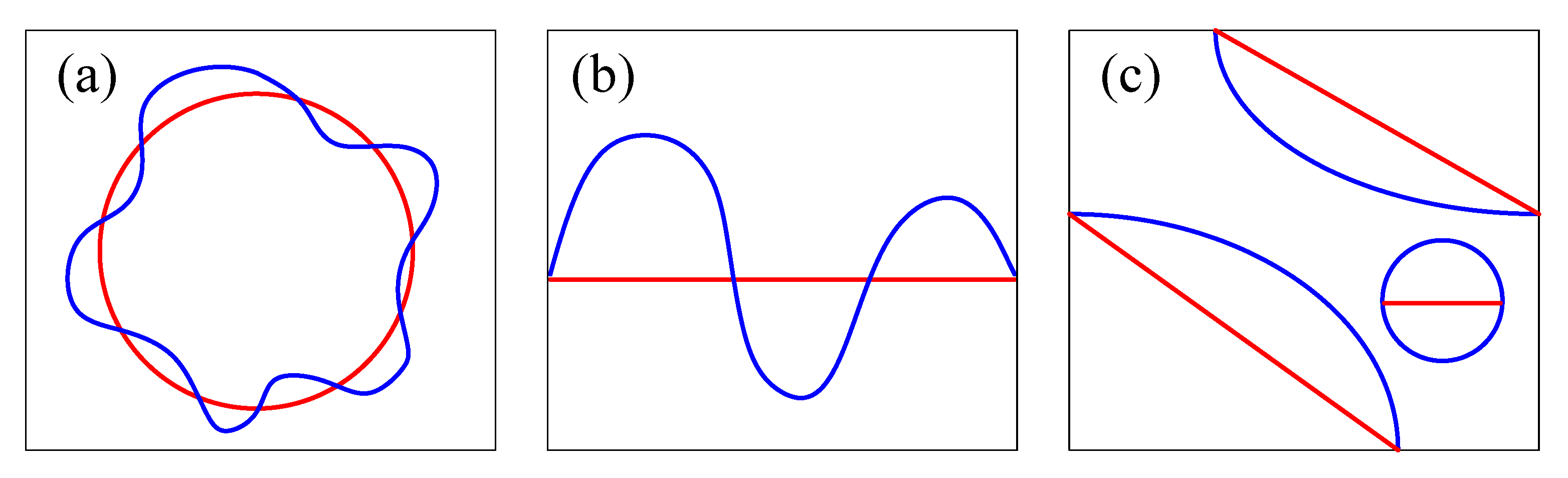
3.2.1. Individual Sinuosity (SIN)
3.2.2. Aggregate Sinuosity (ASIN)
3.2.3. Comprehensive Sinuosity (CSIN)
4. Results and Analysis
4.1. Quantification of Anomalous Circulation States Using ASIN
4.1.1. Correlation between ASIN and Climate Variables
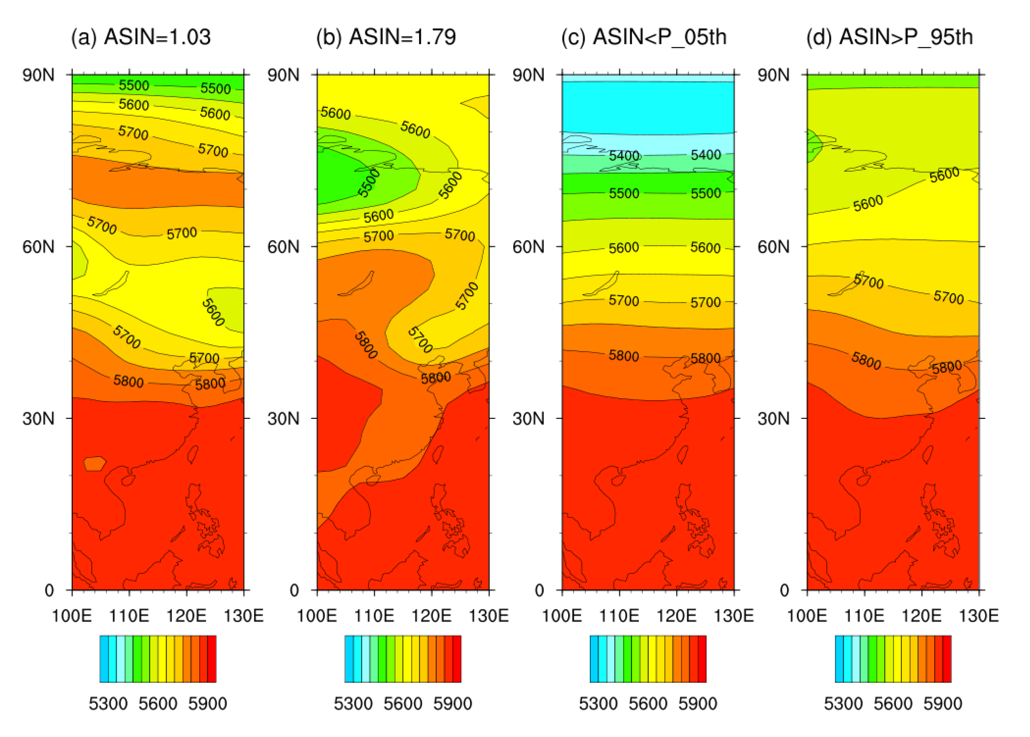
4.1.2. Different Circulation States in August
4.1.3. Sensitivity Testing of the Choice of Different Size Areas
4.2. Influence of Sinuosity at Different Latitudes on SAT in Southeastern China
4.2.1. SIN
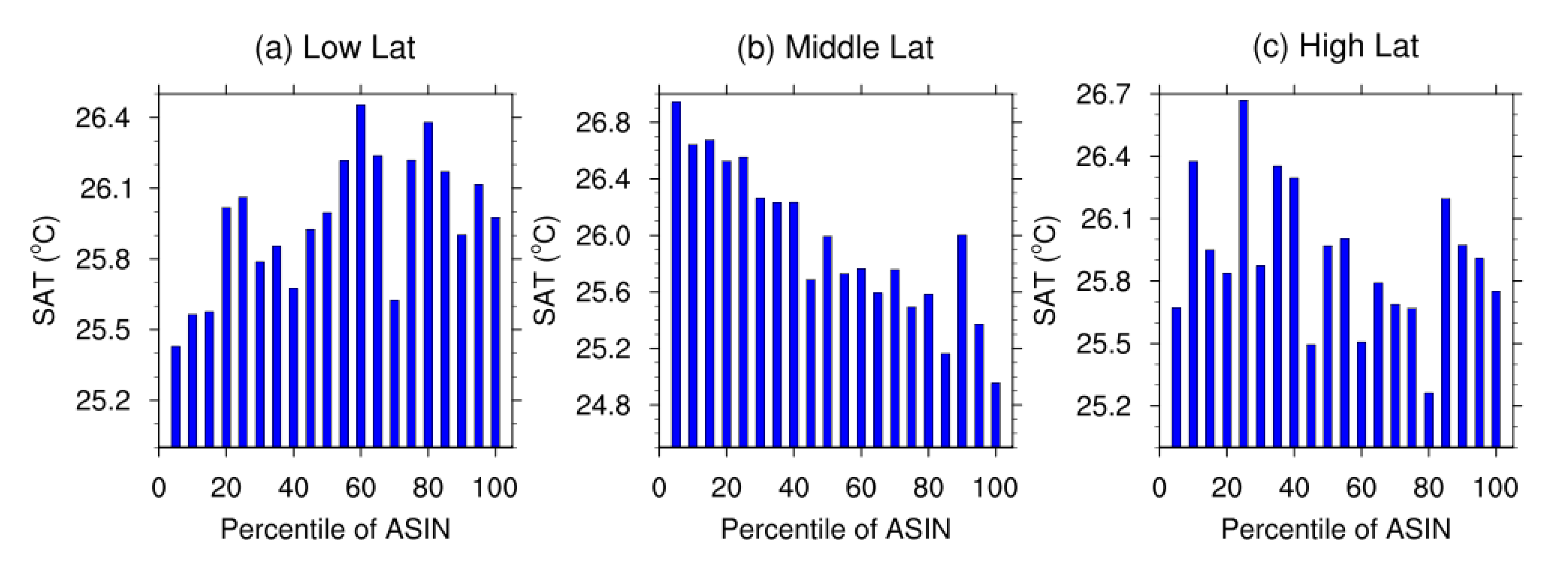
4.2.2. ASIN
4.3. Future Changes of Climate Variables in Southeastern China
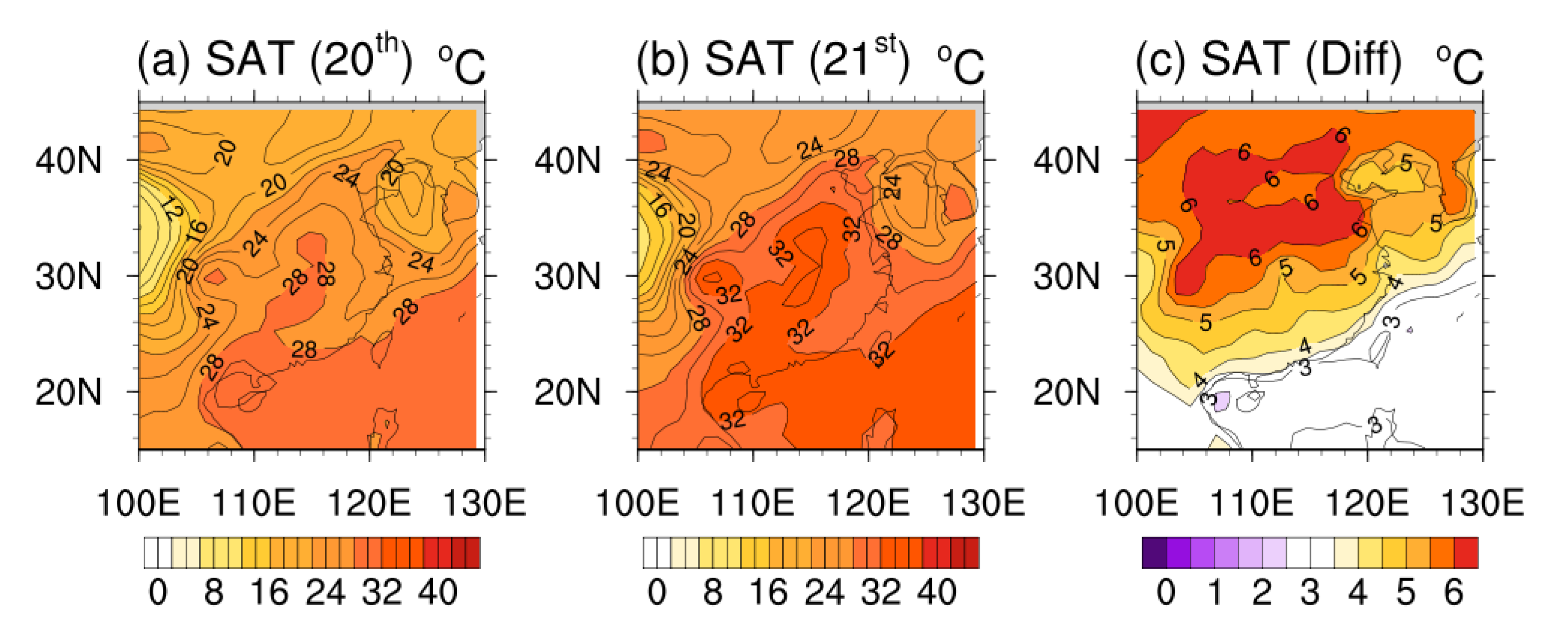
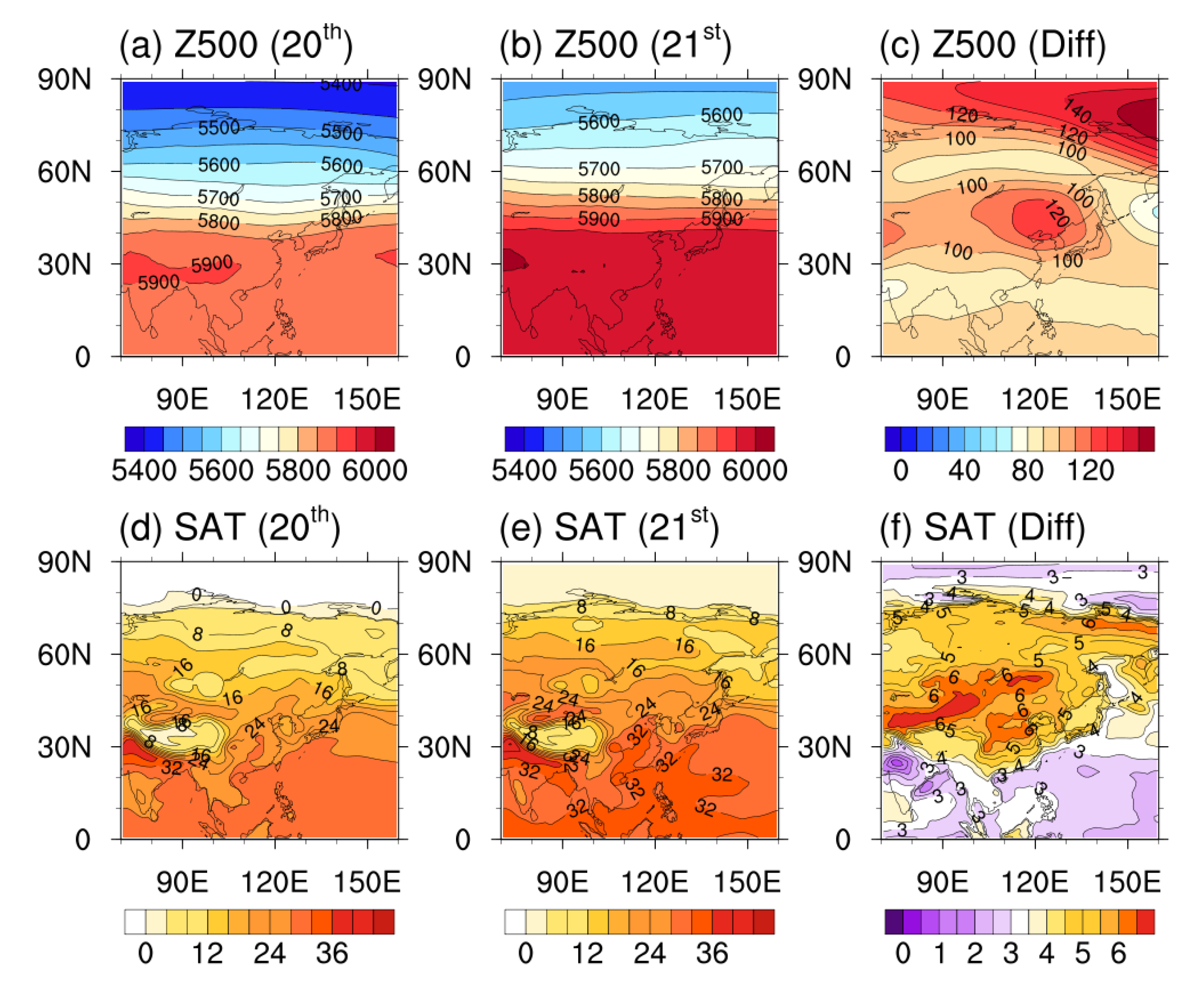
4.3.1. Changes of SATs
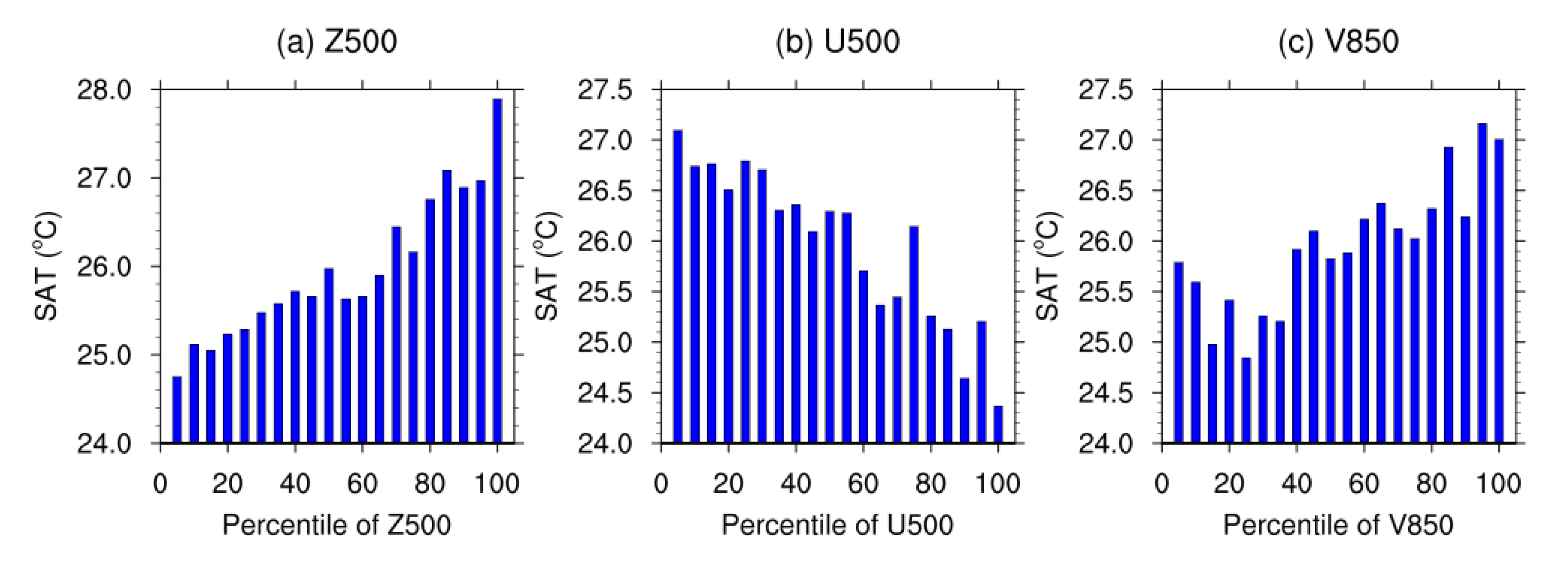
4.3.2. Relationship between Wind, Pressure, and Temperature
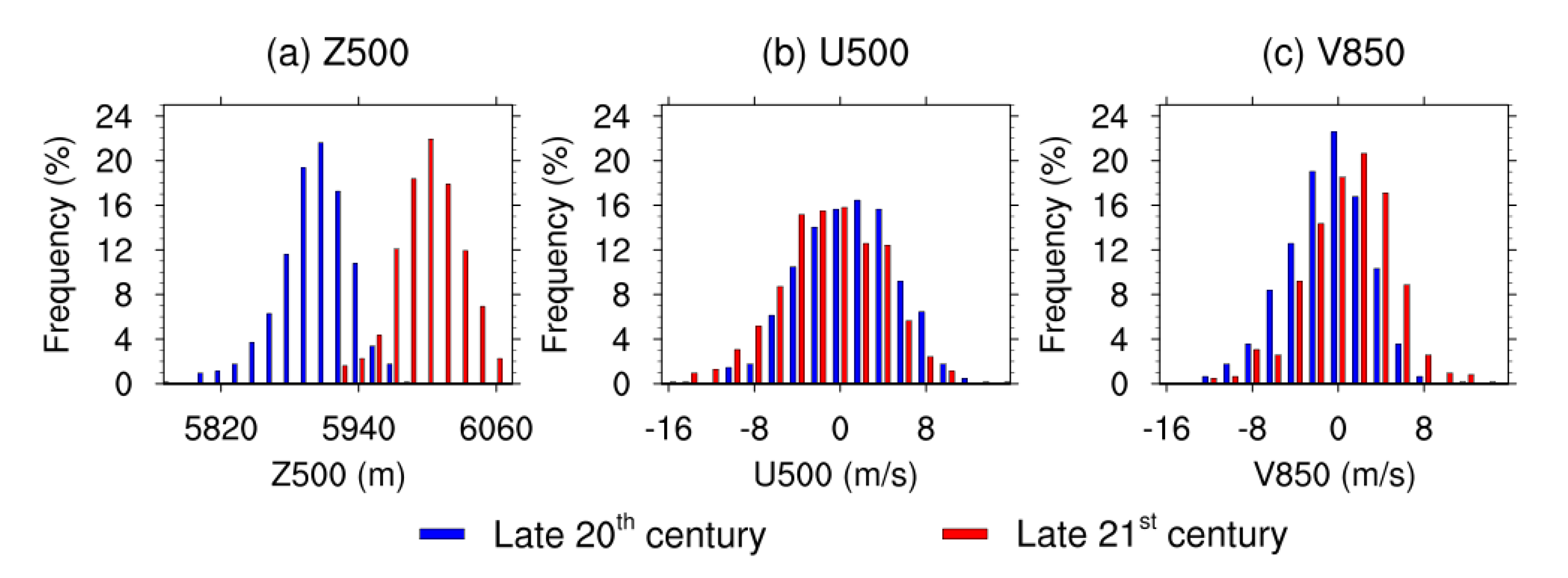
4.3.3. Changes in Wind and Pressure
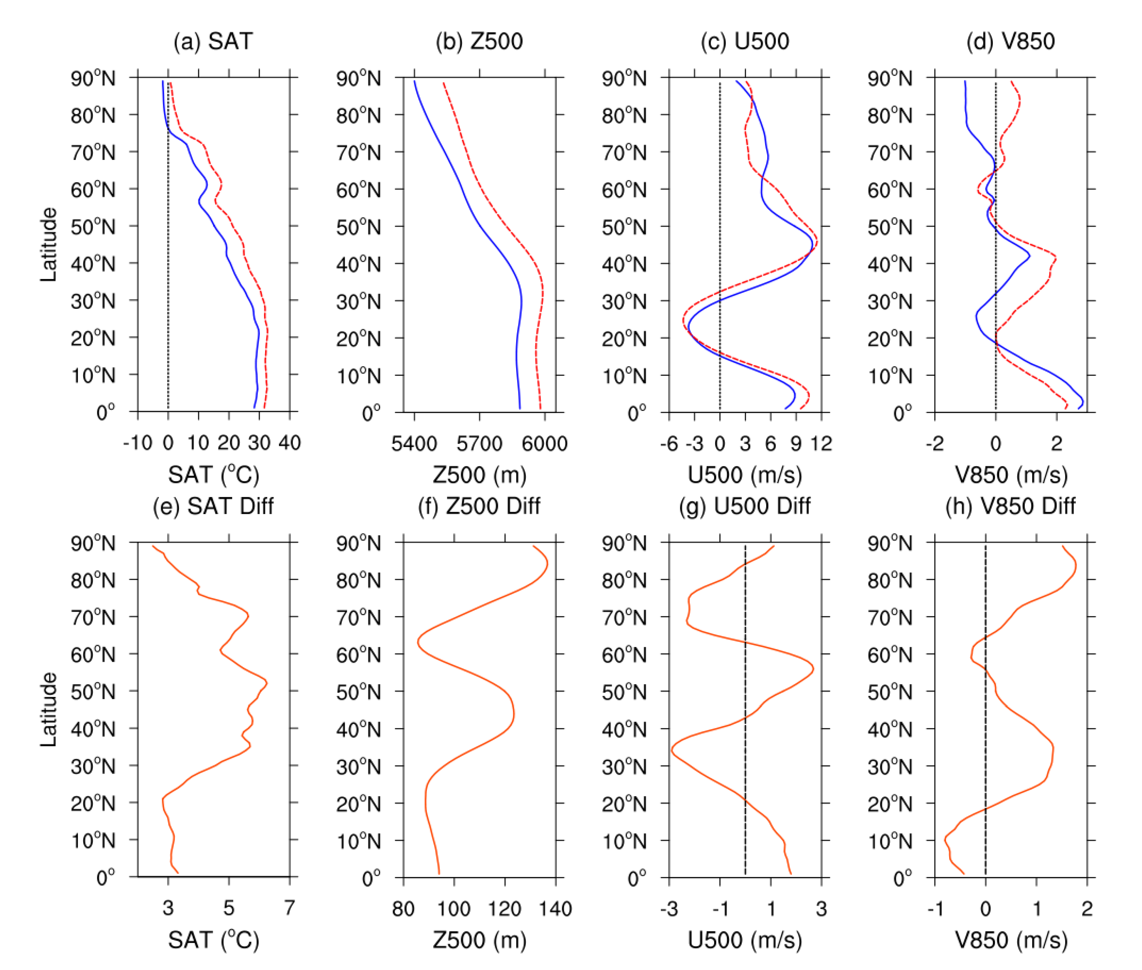
4.4. Distribution Regularities in Different Latitudes for Each Climate Variable
4.4.1. 50° N–60° N
4.4.2. 35° N–50° N
4.4.3. 20° N–35° N
4.4.4. 0° N–20° N
4.5. Distribution Regularities in Different Latitudes for Each Climate Variable
5. Summary and Discussion
- The exceptional circulation states can be quantified by ASIN. The HTEs can more easily appear when ASIN is at its peak.
- Influences of SINs at different latitudes on the SAT of southeastern China differ. The SAT of southeastern China becomes higher with greater ASIN. ASIN in the mid latitudes is the equivalent of a barrier here, which can effectively prevent the cold northern air from going south.
- Projections of future average SAT indicate a significant increase and a northwest–southeast gradient warming in August over southeastern China.
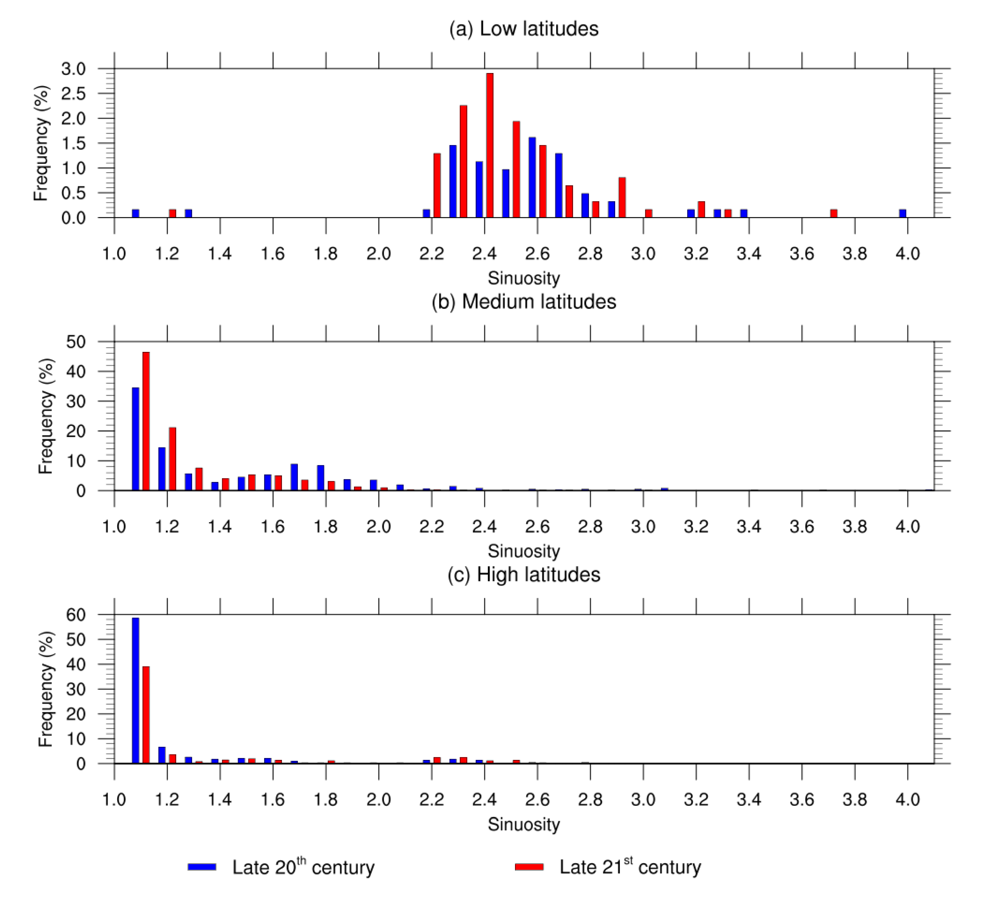
- In the bigger picture, SAT changes in southeastern China can be explained by the CSIN of Z500 isohypses at different latitudes. At the end of the 21st century, Z500 isohypses at different latitudes will obviously have a poleward shift. Moreover, the frequencies of large (small) CSIN at low (mid) latitudes increased.
Author Contributions
Funding
Institutional Review Board Statement
Informed Consent Statement
Data Availability Statement
Acknowledgments
Conflicts of Interest
References
- Meehl, G.A.; Tebaldi, C. More intense, more frequent, and longer lasting heat waves in the 21st century. Science 2004, 305, 994–997. [Google Scholar] [CrossRef] [Green Version]
- Perkins, S.E.; Alexander, L.V.; Nairn, J.R. Increasing frequency, intensity and duration of observed global heatwaves and warm spells. Geophys. Res. Lett. 2012, 39, L20714. [Google Scholar] [CrossRef]
- Wang, H.; Sun, J.; Chen, H.; Zhu, Y.; Zhang, Y.; Jiang, D.; Yang, S. Extreme climate in China: Facts, simulation and projection. Meteorol. Z. 2012, 21, 279–304. [Google Scholar] [CrossRef]
- Trenberth, K.E.; Dai, A.; van der Schrier, G.; Jones, P.D.; Barichivich, J.; Briffa, K.R.; Sheffield, J. Global warming and changes in drought. Nat. Clim. Chang. 2014, 4, 17–22. [Google Scholar] [CrossRef]
- Wang, H.; Chen, H. Understanding the recent trend of haze pollution in eastern China: Roles of climate change. Atmos. Chem. Phys. Discuss. 2016, 1–18. [Google Scholar] [CrossRef] [Green Version]
- Christensen, J.H.; Hewitson, B.; Busuioc, A.; Chen, A.; Gao, X.; Held, I.; Jones, R.; Kolli, R.K.; Kwon, W.T.; Laprise, R.; et al. Regional climate projections. In Climate Change 2007: The Physical Science Basis; Solomon, S., Ed.; Cambridge University Press: Cambridgeshire, UK, 2007; pp. 847–940. [Google Scholar]
- Christensen, J.H. Coauthors. Climate phenomena and their relevance for future regional climate change. In Climate Change 2013: The Physical Science Basis; Stocker, T.F., Ed.; Cambridge University Press: Cambridgeshire, UK, 2013; pp. 1217–1308. [Google Scholar] [CrossRef]
- Min, S.K.; Kim, Y.H.; Kim, M.K.; Park, C. Assessing human contribution to the summer 2013 Korean heat wave in Explaining Extreme Events of 2013 from a Climate Perspective. Bull. Amer. Meteorol. Soc. 2014, 95, S48–S51. [Google Scholar]
- Min, S.K.; Son, S.W.; Seo, K.H.; Kug, J.S.; An, S.I.; Choi, Y.S.; Lee, M.I. Changes in weather and climate extremes over Korea and possible causes: A review. Asia-Pac. J. Atmos. Sci. 2015, 51, 103–121. [Google Scholar] [CrossRef]
- Wei, J.; Yang, H.; Sun, S.Q. Relationship between the anomaly longitudinal position of subtropical high in the western Pacific and severe hot weather in North China in summer. Acta. Meteorol. Sin. 2004, 62, 308–316. (In Chinese) [Google Scholar]
- Maheras, P.; Flocas, H.; Tolika, K.; Anagnostopoulou, C.; Vafiadis, M. Circulation types and extreme temperature changes in Greece. Clim. Res. 2006, 30, 161–174. [Google Scholar] [CrossRef]
- Gershunov, A.; Cayan, D.R.; Iacobellis, S.F. The great 2006 heat wave over California and Nevada: Signal of an increasing trend. J. Clim. 2009, 22, 6181–6203. [Google Scholar] [CrossRef] [Green Version]
- Sun, J.H.; Chen, H.; Zhao, S.W.; Zeng, Q.C.; Xie, Z.; Cui, J.L.; Liu, H.T. A study on the severe hot weather in Beijing and North China. Part II. Simulation and analysis. Clim. Environ. Res. 1999, 4, 334–345. (In Chinese) [Google Scholar]
- Black, E.; Blackburn, M.; Harrison, G.; Hoskins, B.; Methven, J. Factors contributing to the summer 2003 European heatwave. Weather 2004, 59, 217–223. [Google Scholar] [CrossRef]
- Zhang, M.; Fu, G.; Guo, J. Diagnostical analysis of an extreme high-temperature weather event in North China on 15 July, 2002. J. Ocean. Univ. China. 2005, 35, 183–188. (In Chinese) [Google Scholar]
- Zaitchik, B.F.; Macalady, A.K.; Bonneau, L.R.; Smith, R.B. Europe’s 2003 heat wave: A satellite view of impacts and land–atmosphere feedbacks. Int. J. Climatol. 2006, 26, 743–769. [Google Scholar] [CrossRef]
- Zhang, Y.; Zhang, S. Causation analysis on a largescale continuous high temperature process occurring in North China plain. Meteorol. Mon. 2010, 36, 8–13. (In Chinese) [Google Scholar]
- Ziv, B.; Saaroni, H.; Alpert, P. The factors governing the summer regime of the eastern Mediterranean. Int. J. Climatol. 2004, 24, 1859–1871. [Google Scholar] [CrossRef]
- Harpaz, T.; Ziv, B.; Saaroni, H.; Beja, E. Extreme summer temperatures in the east Mediterranean—Dynamical analysis. Int. J. Climatol. 2014, 34, 849–862. [Google Scholar] [CrossRef]
- Sun, J.; Wang, H. Regional Difference of Summer Air Temperature Anomalies in Northeast China and Its Relationship to Atmospheric General Circulation and Sea Surface Temperature. Chin. J. Geophys. CH. 2006, 49, 588–598. [Google Scholar] [CrossRef]
- Sun, J.; Wang, H.; Yuan, W. Decadal variations of the relationship between the summer North Atlantic Oscillation and middle East Asian air temperature. J. Geophys. Res. Atmos. 2008, 113, D15107. [Google Scholar] [CrossRef]
- Sun, J.; Wang, H.; Wei, A.Y. Decadal Variability of the Extreme Hot Event in China and Its Association with Atmospheric Circulations. Clim. Environ. Res. 2011, 16, 199–208. (In Chinese) [Google Scholar]
- Cattiaux, J.; Peings, Y.; Saint-Martin, D.; Trou-Kechout, N.; Vavrus, S.J. Sinuosity of midlatitude atmospheric flow in a warming world. Geophys. Res. Lett. 2016, 43, 8259–8268. [Google Scholar] [CrossRef] [Green Version]
- Vavrus, S.J.; Wang, F.; Martin, J.E. Changes in North American Atmospheric Circulation and Extreme Weather: Influence of Arctic Amplification and Northern Hemisphere Snow Cover. J. Clim. 2017, 30, 4317–4333. [Google Scholar] [CrossRef]
- Peings, Y.; Cattiaux, J.; Vavrus, S.; Magnusdottir, G. Late twenty-first-century changes in the midlatitude atmospheric circulation in the CESM large ensemble. J. Clim. 2017, 30, 5943–5960. [Google Scholar] [CrossRef] [Green Version]
- Di Capua, G.; Coumou, D. Changes in meandering of the Northern Hemisphere circulation. Environ. Res. Lett. 2016, 11, 094028. [Google Scholar] [CrossRef]
- Seneviratne, S.I. Coauthors. Changes in climate extremes and their impacts on the natural physical environment. In Managing the Risks of Extreme Events and Disasters to Advance Climate Change Adaptation; Field, C.B., Ed.; Cambridge University Press: Cambridgeshire, UK, 2012; pp. 109–230. [Google Scholar]
- Lucas, C.; Timbal, B.; Nguyen, H. The expanding tropics: A critical assessment of the observational and modeling studies. WIREs. Clim. Chang. 2013, 5, 89–112. [Google Scholar] [CrossRef]
- Kanamitsu, M.; Ebisuzaki, W.; Woollen, J. NCEP–DOE AMIP-II Reanalysis (R-2). Bull. Amer. Meteorol. Soc. 2002, 83, 1631–1643. [Google Scholar] [CrossRef]
- Xu, Y.; Gao, X.; Shen, Y.; Xu, C.; Shi, Y.; Giorgi, F. A Daily Temperature Dataset over China and Its Application in Validating a RCM Simulation. Adv. Atmos. Sci. 2009, 26, 763–772. [Google Scholar] [CrossRef]
- Taylor, K.E.; Stouffer, R.J.; Meehl, G.A. An overview of CMIP5 and the experiment design. Bull. Amer. Meteorol. Soc. 2012, 93, 485–498. [Google Scholar] [CrossRef] [Green Version]
- Zhao, S.; He, W. Performance evaluation of Chinese air temperature simulated by Beijing Climate Center Climate System Model on the basis of the long-range correlation. Acta. Phys. Sin. 2014, 63, 209201. (In Chinese) [Google Scholar]
- Zhao, S.; He, W. Performance evaluation of the simulated daily average temperature series in four seasons in China by Beijing Climate System Model. Acta. Phys. Sin. 2015, 64, 049201. (In Chinese) [Google Scholar]
- Tian, Y.Z.; Chen, S.P.; Yue, T.X.; Zhu, L.F.; Wang, Y.A.; Fan, Z.M.; Ma, S.N. Simulation of Chinese population density based on land use. Acta. Geogr. Sin. 2004, 59, 283–292. (In Chinese) [Google Scholar]
- Ge, M.L.; Feng, Z.M. Population distribution of China based on GIS: Classification of population densities and curve of population gravity centers. Acta. Geogr. Sin. 2009, 64, 202–210. (In Chinese) [Google Scholar]
- Wang, Z.F.; Chen, P. Unbalanced economic development and coordinated development of eastern and western China. J. Jishou. Univ. 2010, 31, 111–115. [Google Scholar]
- Chen, R.; Lu, R. Comparisons of the Circulation Anomalies Associated with Extreme Heat in Different Regions of Eastern China. J. Clim. 2015, 28, 5830–5844. [Google Scholar] [CrossRef]
- Zhang, Q.; Chen, L. Variations of dryness and wetness in China during 1951–1980. Sci. Atmos. Sin. 1991, 15, 72–81. (In Chinese) [Google Scholar]
- Wei, K.; Chen, W. Climatology and trend of high temperature extremes across China in summer. Atmos. Oceanic. Sci. Lett. 2009, 2, 153–158. [Google Scholar]
- Zheng, J.; Yin, Y.; Li, B. Scheme of climate regionalization in China. Acta. Geogr. Sin. 2010, 65, 3–13. (In Chinese) [Google Scholar]
- Barnes, E.A. Revisiting the evidence linking Arctic amplification to extreme weather in midlatitudes. Geophys. Res. Lett. 2013, 40, 4734–4739. [Google Scholar] [CrossRef]
- Quante, M.; Colijn, F.; Sterl, A. North Sea Region Climate Change Assessment; Springer International Publishing: Berlin, Germany, 2016. [Google Scholar]
- Oard, M.J. A method for predicting chinook winds east of the Montana Rockies. Weather Forecast 1993, 8, 166–180. [Google Scholar] [CrossRef]
- Mercer, A.E.; Richman, M.B.; Bluestein, H.B. Statistical modeling of downslope windstorms in Boulder, Colorado. Weather Forecast 2008, 23, 1176–1194. [Google Scholar] [CrossRef] [Green Version]
- Manton, M.J. Trends in extreme daily rainfall and temperature in Southeast Asia and the South Pacific: 1961–1998. Int. J. Climatol. 2001, 21, 269–284. [Google Scholar] [CrossRef]
- Sheikh, M.M.; Manzoor, N.; Ashraf, J.; Adnan, M.; Collins, D.; Hameed, S.; Manton, M.J.; Ahmed, A.U.; Baidya, S.K.; Borgaonkar, H.P. Trends in extreme daily rainfall and temperature indices over South Asia. Int. J. Climatol. 2015, 35, 1625–1637. [Google Scholar] [CrossRef]
- De Luca, D.L.; Petroselli, A.; Galasso, L. A Transient Stochastic Rainfall Generator for Climate Changes Analysis at Hydrological Scales in Central Italy. Atmosphere 2020, 11, 1292. [Google Scholar] [CrossRef]


| Climate Variable | Daily Variation | Climatological Mean | Interannual Variability |
|---|---|---|---|
| SAT | 0.24 | 0.75 | 0.41 |
| Z500 | 0.35 | 0.71 | 0.58 |
| U500 | −0.24 | −0.78 | −0.51 |
| V850 | 0.12 | 0.43 | 0.23 |
| Isohypse | 5950 | 5900 | 5850 | 5800 | 5750 | 5700 | 5650 | 5600 | 5550 | 5500 | 5450 | 5400 | 5350 |
|---|---|---|---|---|---|---|---|---|---|---|---|---|---|
| r values | 0.01 | 0.20 | 0.04 | −0.21 | −0.13 | −0.02 | 0.02 | 0.15 | 0.11 | 0.03 | −0.07 | −0.07 | −0.05 |
Publisher’s Note: MDPI stays neutral with regard to jurisdictional claims in published maps and institutional affiliations. |
© 2021 by the authors. Licensee MDPI, Basel, Switzerland. This article is an open access article distributed under the terms and conditions of the Creative Commons Attribution (CC BY) license (https://creativecommons.org/licenses/by/4.0/).
Share and Cite
Wang, Y.; Wang, F.; Sun, X. Sinuosity of Atmospheric Circulation over Southeastern China and Its Relationship to Surface Air Temperature and High Temperature Extremes. Atmosphere 2021, 12, 1139. https://doi.org/10.3390/atmos12091139
Wang Y, Wang F, Sun X. Sinuosity of Atmospheric Circulation over Southeastern China and Its Relationship to Surface Air Temperature and High Temperature Extremes. Atmosphere. 2021; 12(9):1139. https://doi.org/10.3390/atmos12091139
Chicago/Turabian StyleWang, Yongdi, Fei Wang, and Xinyu Sun. 2021. "Sinuosity of Atmospheric Circulation over Southeastern China and Its Relationship to Surface Air Temperature and High Temperature Extremes" Atmosphere 12, no. 9: 1139. https://doi.org/10.3390/atmos12091139
APA StyleWang, Y., Wang, F., & Sun, X. (2021). Sinuosity of Atmospheric Circulation over Southeastern China and Its Relationship to Surface Air Temperature and High Temperature Extremes. Atmosphere, 12(9), 1139. https://doi.org/10.3390/atmos12091139