Abstract
As the aviation industry has entered a critical period of development, the demand for Automatic Dependent Surveillance Broadcast (ADS-B) technology is becoming increasingly urgent. Real-time detection of aviation wind field information and the early warning of wind field shear by atmospheric sounding system are two important factors related to the safe operation of aviation and airport. According to the advantages of ADS-B and Mode S data, this paper uses the Meteo-Particle (MP) model proposed by Sun et al., in their previous research to retrieve high-altitude wind field. Comparing the precision and accuracy of wind field retrieved results, and the optimization parameters of MP model suitable for meteorological model are further studied. To solve the problem of incomplete wind field coverage obtained by retrieval, an extrapolation algorithm of wind field is proposed. The results show that: (1) a comprehensive evaluation index is introduced, which can more effectively evaluate the comprehensive difference of wind field retrieval results in wind speed and direction. (2) The adaptability results of MP model in different periods and altitudes provide some reference for the research of other scholars. (3) The new parameter setting can improve the accuracy of the retrieved results, and the appropriate extrapolation of wind field fills in the blank part of aviation and meteorology.
1. Introduction
The distribution of high-altitude wind fields affects the daily operation of aircraft, and its unprovoked changes often lead to air traffic accidents. At the same time, the saturated air routes also force the Civil Aviation Authority and the Air Traffic Control Bureau to control the air traffic flow to ensure the basic safety of flight. With the rapid increase of travel frequency and the increasing congestion of air traffic, researchers need to adopt measures to improve the aircraft volume ratio in the airspace. Accurate and high-precision meteorological information, especially the changes in the wind field, can effectively reduce the flight interval of the aircraft and expand the capacity over the airport [1,2]. The weather conditions on the route are the main factors affecting flight operation and scheduling. Some weather professionals, though, can provide some low-level wind information from weather radar, lidar, etc., or use weather forecasting models to reanalyze the data. Low-level wind information may also be obtained from telescopes (there are some methods based on the analysis of the optical distortions to detect turbulent layers, inversion layers, low-level jets) [3,4]. However, this information is relatively smooth wind data, there are no wind field details required by ATC [5]. Compared with other meteorological observation data, the high-resolution observation data of high-altitude wind fields is especially scarce, and the existing data are far from enough to serve as reference data for air traffic control. Therefore, the technology of secondary radar and Automatic Dependent Surveillance Broadcast need to be developed rapidly to make up for this deficiency.
As a mature and reliable surveillance technology, the Secondary Surveillance Radar (SSR) has been widely used in air traffic control systems. However, the SSR system has some disadvantages, such as low update frequency, large monitoring error, and high cost, complex installation and maintenance, and so on [6,7,8]. Automatic Dependent Surveillance Broadcasting (ADS-B) is a new type of air traffic control and monitoring technology based on the Global Navigation Satellite System (GNNS). The application of ADS-B is an important technical means to ensure flight safety, improve operational efficiency, increase air traffic flow, and reduce construction investment. ADS-B and SSR need to complement each other and gradually realize the transition from secondary radar to ADS-B [9,10,11].
In recent years, with the rapid development of the civil aviation transport industry and the rapid increase in the number of flights, aircraft performance has been continuously improved. This further aggravates the impact of important weather on the safety and efficiency of flight operation and makes the impact of important weather on flight operation more significant [12,13]. Therefore, the research on the wind field in the high-altitude area has become an urgent need in the field of civil aviation. In order to solve this problem effectively, this paper improves the existing retrieval method of high-altitude wind fields on the basis of the study of high-altitude wind fields at the present stage. Based on the previous research of Sun et al., this paper further explores the applicability of the Meteo-Particle (MP) model at different height levels and combining with meteorological knowledge. Its parameters can be adjusted to improve its scope of application and accuracy, thus as to improve the accuracy and stability of the wind field. This method can provide real-time and high-altitude wind field observation for aircraft with higher time resolution, wide range, and better fineness. At the same time, the results of wind field extrapolation can provide data reference for aviation, meteorology, and other fields, which is convenient for further research.
The main contributions of this paper are as follows:
- (1)
- A scheme is proposed to verify the accuracy of wind field retrieval.
- (2)
- The applicability of instantaneous wind field data estimated by linear extrapolation model in wind field retrieval verification is studied.
- (3)
- Summarize the differences of MP models at different altitudes.
- (4)
- Find the MP model parameters suitable for the aviation weather field.
- (5)
- The extrapolation method of the retrieval of the high-altitude wind field is studied, and the complete wind field data are obtained.
The rest of this article is structured as follows. The next section introduces the research data set in this paper and gives an overview of the data processing methods. The third part introduces the theoretical algorithm of wind field retrieval, including the derivation of wind vector, the principle of MP model, and the verification scheme of retrieval results. The fourth part is the research experiment of this paper, which mainly includes the wind field retrieval and verification experiment, the applicability experiment of the linear difference model, the different experiment of the MP model in each height layer, the improvement of the model, and the wind field extrapolation experiment. The final two parts give the conclusion of this paper.
2. Materials and Processing Methods
2.1. Study Data
ADS-B data has the characteristics of high precision and fast updating speed. The system integrates a variety of advanced and complex technologies, such as satellite navigation, communication, aircraft equipment, ground equipment, and so on. It is also a modern meteorological information perception and sharing technology with a high update rate and high precision. At the same time, there are still some civil aircraft that are not equipped with ADS-B airborne response equipment, thus there are some problems with missing data. As a mature and reliable monitoring technology, SSR has been widely used in air traffic control systems, but its data have the disadvantages of low update frequency, large monitoring error, and high cost [14]. Therefore, this paper will take advantage of these two kinds of data at the same time and give full play to their complementary advantages to retrieve the high-altitude wind field.
ADS-B data begins with 17 downlink formats, with a total of 112 bits, which transmits the aircraft position, speed, and other information through Mode S extension (1090 MHz). The main parameters include ICAO address, air position information, altitude information, and airspeed. Typically, ADS-B data are sent once or twice a second. Mode S data begins with a format of 20 or 21 in the following uplink format, with a total of 112 bits. The principal parameters include ICAO address, BDS4,0 height, BDS5,0 heading angle, ground speed, true airspeed, and Mach number [15].
Part of the experimental data used in this paper was received by ADS-B/Mode S receiver (longitude: 4.37° E, latitude: 51.99° N) installed at Delft University of Technology [16,17], which can be obtained at https://doi.org/10.6084/m9.figshare.6970403.v1, 16 November 2020. The data used for wind field retrieval included ADS-B data and Mode S data at 09:00–10:00 UTC on 1 January 2018 and a half an hour before and after 00:00, 06:00, 12:00, and 18:00 UTC on 1 January 2018. The rest of the data comes from the OpenSky platform [18,19], which can be obtained at http://www.opensky-network.org, 20 November 2020, and the differences between ADS-B and Mode S data are shown in Table 1.

Table 1.
Comparison of monitoring means.
The reference data used in this paper are the ERA5 reanalysis data from the European Centre for Medium-Range Weather Forecasts (ECMWF), including instantaneous wind data at 00:00, 06:00, 12:00, and 18:00 UTC on 1 January 2018, with a spatial resolution of 0.25°. ECMWF ERA5 integrates a large number of historical observations into global estimates using advanced modeling and data assimilation systems. It provides the estimation of atmospheric parameters with a horizontal grid accuracy of 31 km and an output frequency of hourly. At present, some studies have given the vertical distribution of wind speed, which shows that the reanalyzed wind data of NCEP/NCAR et al., were robust [20]. However, as the comparative data of this paper, ERA5 has some defects, which are explained in this paper. Firstly, the horizontal grid resolution (31 km) of ERA5 is still limited, and the rough grid resolution will lead to the difference in the evaluation results in this paper. Secondly, because the grid of ECMWF ERA5 weather forecast model is fixed and the data update interval is large, the data set obtained is usually too smooth, and there is no local change of wind field retrieved in this paper. Finally, the time resolution of ERA5 is limited, which can only provide instantaneous parameters of wind field-related information and cannot correspond to the experimental data one by one. However, it is difficult to directly detect the wind field information in the corresponding area due to its special geographical location. Moreover, the existing wind field data have some shortcomings, such as small monitoring range, low spatial resolution, and so on. The real verification data of this experiment are difficult to obtain and lack of factual basis. Therefore, in order to initially evaluate the accuracy of the wind field retrieval method, ERA5 reanalysis data has to be used as reference data in this paper, which is very important for the optimization of MP model.
2.2. Data Processing
Data decoding. The received ADS-B source data need to be decoded for further application. In this paper, the pyModeS of Python [21] is used to decode the 28-bit hexadecimal ADS-B and Mode S source data directly to obtain time, latitude, and longitude, altitude, ground speed, vacuum speed, Mach number, indicated airspeed, magnetic heading, and other information.
Data screening. This paper sifts and sorts the data from the Delft University of Technology and its surrounding areas, centering on the location of the receiver (longitude: 4.37° E, latitude: 51.99° N), within a radius of 300 km and an altitude of 5 km to 12 km.
3. Wind Field Retrieval and Verification Indexes
3.1. Calculation of Wind Vector
There is no absolute wind speed and direction information in the source data of ADS-B and Mode S, thus it was necessary to calculate the wind vector according to the kinematic relationship of the aircraft. In theory, the airspeed of an airplane is equal to the ground speed under the ideal condition of no wind. In fact, due to the existence of the wind, the airspeed collected by the sensors will change with the wind. When the wind is downwind, the airflow is in the same direction as the aircraft, and the collected airspeed becomes smaller, that is, the airspeed is less than the ground speed. When the airflow is opposite to the aircraft in the headwind, the collected airspeed becomes larger, that is, the airspeed is greater than the ground speed. Then, the wind information is calculated according to this internal relationship. The relationship among airspeed vector, ground speed vector, and wind vector is shown in Figure 1, and the relationship between them can be simplified into Equation (1). In the actual calculation, in order to simplify the calculation, it needs to be decomposed into a horizontal component and a vertical component, as shown in Equations (2) and (3) [22,23,24,25].
where, is the ground speed vector, is the airspeed vector and is the wind speed vector.
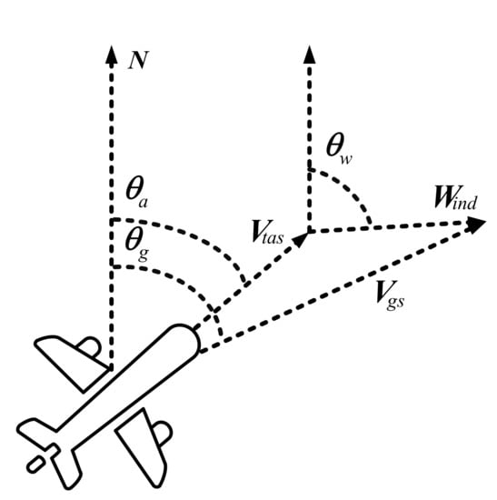
Figure 1.
Vector relation of aircraft motion.
3.2. Structure of Wind Field
The wind field information obtained from the ADS-B and Mode S data is almost all distributed on the air route, while there is still a lack of wind observation in some areas outside the route. Therefore, in order to calculate the wind field in the area with low measured density, the MP model proposed by Junzi Sun et al., was used in this paper to extend the wind vector information to obtain more abundant wind field data [17]. This paper only studies the applicability and improvement measures of the MP model for wind field retrieval. In order to make the results independent and try to minimize the influence of irrelevant factors, this paper makes some adjustments on the basis of the original MP model in the course of the experiment. The specific adjustments are as follows: (1) reduce the temperature estimation module, only focus on the wind field retrieval module. (2) The confidence part is removed, and the difference of confidence of each point is not considered temporarily. The MP model is based on the following three assumptions:
- The true state of the wind is geographically stable at the level of dozens of kilometers. Then the distribution of wind fields in other locations can be calculated from the observed data in the neighborhood.
- The true state of the wind is stable at the level of a few minutes. This assumption is usually correct because aircraft try to avoid extreme atmospheric conditions.
- The sudden error rate of a single aircraft observation will not be too high.
This paper discusses the MP model of Sun in order to help readers better understand the model and the work of this article. In order to better reflect the details of the optimization of the parameters in the latter part of the article, this paper gives a brief overview of the MP model proposed by Sun et al., according to our understanding. The key algorithms of the model and the model parameters involved later are explained, which is convenient for readers to understand and think. For the more detailed MP model algorithm and implementation steps, readers can refer to the relevant literature [17], in which there is a detailed formula expression and model description. This section mainly introduces the key algorithms of the MP model and combs its implementation process [17]. Figure 2 is the flow chart of the MP model combed in this paper.
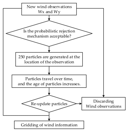
Figure 2.
Flow chart of MP model.
3.2.1. Probabilistic Rejection Mechanism
In order to reduce the impact of the abrupt error rate of aircraft observation on the results, the probabilistic rejection mechanism was adopted. For the new measured value , the probability density function will be constructed based on the current measured value, and the mean and variance and of the particles of the same height near it will be calculated. The probability density function is shown in Equation (4). Then any new observed sample will be accepted with the probability of .
where, , , is the control parameter.
3.2.2. Random Walks Model
In order to expand the wind field information, the random walk model is adopted. N particle objects with wind vector state are generated at the observed position, and each particle follows a different model to propagate and attenuate over time. The random walk model is shown in Equations (5) and (6).
where represents the current moment and represents the next moment, and are the horizontal and vertical components of the wind vector, respectively. In the horizontal position, the horizontal component of the wind performs a random walk with a small bias along the direction of the wind with a proportional coefficient , and can control the propagation direction. In the vertical direction, the propagation follows the zero-mean Gaussian walk.
Each particle generated in the random walk model is assigned an age parameter with an initial value of zero, and the age of the particle grows with each step of particle propagation. At the end of each update, all current particles are resampled. First, the particles propagated outside the edge region are eliminated, and the age probability of the remaining particles is calculated, as defined in Equation (7). Finally, the particles with high age probability are left.
where, is the age of the particle and is the control parameter.
3.2.3. Gridding of Wind Information
The wind vector of each grid point consists of the weighted values of adjacent particles, and the weight of each particle depends on the distance from the current position of the particle to the grid point, , and the distance from its original position, . The weight values of each factor are shown in Equations (8) and (9). The weight of each particle is determined by the above two factors, thus the total weight of the particle is defined as Equation (10).
Therefore, the wind vector of each grid point can be calculated by Equation (11).
where and are different factor weights, is the control parameter and is the total weight of particles.
3.2.4. Verification Indexes
In order to quantitatively measure the error of wind field retrieval, this paper introduces the evaluation indexes, analyzes the error size and error source from many aspects, and then puts forward the corresponding model improvement method.
- Direct evaluation index
The direct evaluation index in this paper includes amplitude difference and angle difference, in which amplitude difference refers to the difference of wind speed and angle difference refers to the difference of wind direction, as defined in Equations (12) and (13).
- Regression evaluation index
The regression evaluation indexes in this paper include average mean absolute error (), root mean square error (), Pearson correlation coefficient (), and cosine similarity coefficient (), whose definitions are as follows.
- Comprehensive evaluation index
Combined with the characteristics of wind field retrieval from ADS-B and Mode S data, its high-precision data makes the wind field have more details than the ERA5 data. By comparing the experimental results, it was found that there was sometimes a big difference between and , which made it impossible to judge the results. Therefore, this paper studies the difference between them from the definition and nature of the above two indicators. In theory, a vector is a quantity with both size and direction. Judging whether the two vectors are similar, only considering the size or direction may lead to errors in the evaluation of the model. Therefore, this paper attempts to combine these two methods to define a mixed similarity model. This index can measure not only the deviation of the two vectors in the direction but also the deviation of the distance of the two vectors, which makes the measurement of the results more scientific and reasonable [26,27,28]. In this paper, the mixed model is used to improve the calculation of similarity measurement, and the weight parameters are used to synthesize the Pearson correlation coefficient and cosine similarity. In the similarity calculation of the mixed model, a weight parameter is defined to adjust the proportion of and . The constructed model is shown in Formula (18).
where is the adjustment coefficient, which is given by the empirical value of each experiment. In the process of use, different parameters can be adjusted repeatedly according to the application scenario. In this paper, is set according to experience, and the definition is shown in Formula (19).
4. Experiment and Result Verification
4.1. Retrieval and Verification of the Wind Field
In this paper, ADS-B and Mode S data at 00:00, 06:00, 12:00, and 18:00 UTC on 1 January 2018 were selected for wind field retrieval. It includes the data of half an hour before and after the above four moments, and this experiment uses the data of every 100 s to output a wind field chart. The duration of the input data used has a certain impact on the results, but this effect is beneficial. The increase of real-time length can make the results more accurate, and the model can invert the wind field results from a few minutes to several hours in real-time. However, for the sake of the development of this study and the independence of the results, only short-term and long-term results are reflected in the study. In order to understand the specific distribution of wind speed and direction errors, this paper makes statistics as shown in Figure 3 and Figure 4 [29]. At the same time, the variation trend of wind speed and wind direction is relatively consistent, in which the consistency of wind direction is higher than that of wind speed, and the retrieved data reflect more detailed fluctuations. There are some large abrupt changes in the wind speed, which may be outliers or normal abrupt changes in wind speed, but the specific reasons need to be further studied. A uniform grid point with a horizontal resolution of 60 km, vertical resolution of 1 km, and total specification of 600 × 600 × 12 is established in space. Figure 5 shows the retrieval of the wind field from 17:59:10 to 18:00:50. In order to evaluate the accuracy of the retrieved wind field and the MP model, the instantaneous wind in the ECMWF ERA5 reanalysis data is selected as the reference data. First of all, the detailed distribution of wind field information is compared intuitively, and the ERA5 wind field map at 18:00:00 is obtained after the reference data being grid processed by the method of Section 3.2. A preliminary comparison of the two wind field maps shows that the distribution of the wind field is basically the same. Figure 6 is the wind field distribution map after homogenization, which is the smoothed data and lacks the details of wind field changes. Compared with the retrieved wind field in Figure 5, the latter has higher accuracy and contains more details.
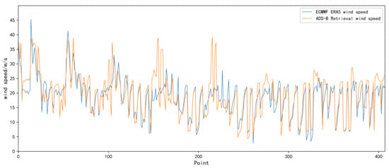
Figure 3.
Contrast of retrieved wind speed and ERA5 wind speed.
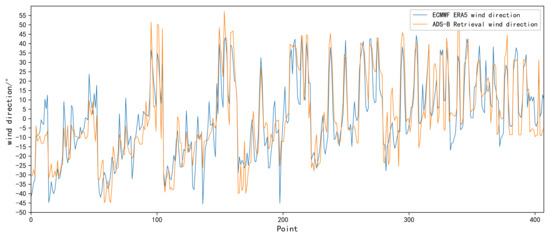
Figure 4.
Contrast of retrieved wind direction and ERA5 wind direction.
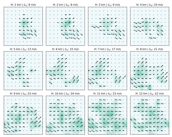
Figure 5.
Retrieval map of wind field during 17:59:10~18:00:50.
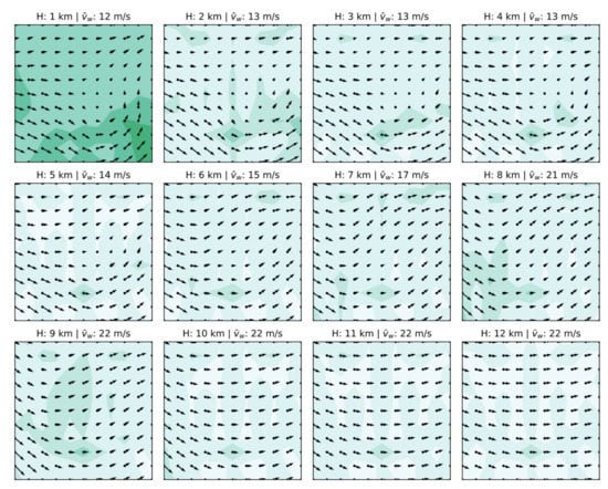
Figure 6.
Wind field map of ECMWF ERA5 data at 18:00:00.
This paper studies the correlation between retrieved wind vector and ERA5 wind vector. In order to better reflect the actual situation of the retrieved error, this paper calculated the relevant evaluation indexes of the error analysis, and the results are shown in Table 2. It can be found that the and components of the wind vector can be retrieved from each set of data, and the overall accuracy is basically above 60%. Among them, the index of the retrieved result around 00:00:00 was less than 40%. Further analysis showed that the main reason was that, compared with other periods, the amount of data around 00:00:00 was very small, and the number of particles in the retrieved only accounted for a small part of the rest of the periods. In general, the MP model has an ideal effect and high accuracy in the retrieval of high-altitude wind fields. By comparing Figure 5 and Figure 6, it is found that the retrieved wind field and the ERA5 wind field have the same wind field profile. The former has a more detailed wind field and more subtle changes, which is of great significance for aviation operation safety and meteorological research. Meanwhile, the distribution of wind speed amplitude difference and wind direction amplitude difference was statistically analyzed, as shown in Figure 7. The results show that the accuracy of wind speed was better than that of wind direction, and the overall effect was ideal. The difference in wind speed was mainly concentrated in (0,4), and the difference in wind direction was mainly distributed in (0,8).

Table 2.
Comparison of and errors in different time periods.
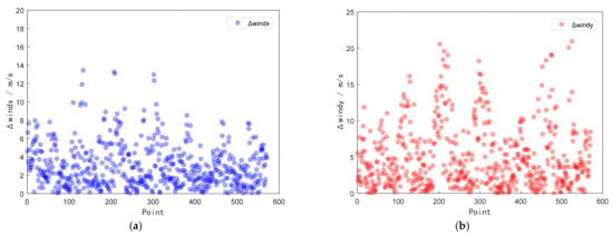
Figure 7.
(a) Scatter distribution of component difference; (b) Scatter distribution of component difference.
4.2. Error Analysis under Linear Interpolation Model
Due to the lack of high-altitude wind field detection data, the time resolution of the wind field data provided by each numerical weather forecast model was basically 6 h, and only included instantaneous data of 00:00, 06:00, 12:00, and 18:00. Therefore, the linear interpolation model was used to fill the ERA5 data set in this paper, which provided a preliminary reference for data in other periods. This is usually correct. Considering that the time span is too large and the wind field changes irregularly, the approximate wind field profile in this time period can only be obtained by using a linear interpolation model for reference.
In this paper, by using the reanalysis data of ECMWF ERA5 of 06:00 and 12:00, the reference data of 9:00~10:00 were calculated through the linear interpolation model, which provides a reference for the result of wind field retrieval in the same period. The error comparison of the reference results is shown in Table 3. The result of the horizontal component is significantly better than that of the vertical component , the index of the former is higher than 70%, and the latter is lower than 50%. It can be seen that the effect of the linear interpolation model is not ideal, but considering the uniformity and smoothness of the ERA5 data, the interpolation results can be used as a preliminary reference and in line with the expected conjecture.

Table 3.
Error comparison of different time periods based on Linear difference Model.
4.3. Error Analysis under Different Periods and Altitudes
The above results show that the number of wind observation samples varies greatly in different periods and different altitudes, thus the accuracy of retrieval is also quite different. Retrieval experiments are carried out in two cases to further analyze the applicability of MP model in different periods and different altitudes [30], and the error results are compared and analyzed.
4.3.1. Error Analysis in Different Periods
Firstly, the data of 00:00, 06:00, 12:00, 18:00 and their nearby periods were selected for wind field retrieval. The results shown in Figure 8a,b are the line charts of the changes in wind speed and wind direction in four periods, respectively. The results showed that the estimated stability of wind speed and direction at 00:00 was low, and there were no retrieval values at many altitudes. This paper analyzes the possible causes of these problems: for the MP model, the more data points, the better the retrieved effect. Compared with other altitudes, the retrieved results at 00:00 may not be ideal because there were too few data points in each height layer, and some height layers even had no observations. In view of the above reasons, the results of the 00:00 period had a great impact on the applicability and accuracy of the analysis model, thus this paper intends to exclude the data results of the 00:00 period.
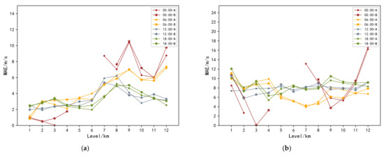
Figure 8.
(a) Line chart of index change of wind speed in each period; (b) Line chart of index change of wind direction in each period.
Figure 8 shows that the accuracy of wind speed retrieval is higher than that of wind direction retrieval. Among them, the change of the index of wind speed in each period was basically the same, and its value was in the range of (1,8). The results of the low layer were better than that of the up layer. The wind direction in [4,14] fluctuated greatly with height, but all fluctuated in an acceptable range. Combined with the distribution of wind speed and direction, the result of 18:00 was the most stable, and the fluctuation was relatively small, while the effect of 00:00 was not good and fluctuated greatly. Through comparison, it was found that 18:00 had the largest amount of data, and the corresponding retrieved result was the most accurate and stable. It can be seen that MP model was not suitable for wind field retrieval with too little data. In general, except for 00:00, the retrieved results of wind speed and direction were ideal and relatively stable. The overall stability was 18:00 > 12:00 > 06:00 > 00:00.
4.3.2. Error Analysis under Different Altitudes
This article also selects the data of 18:00 for wind field retrieval and calculates the distribution of each index at different altitudes. Because the accuracy of the wind field obtained by the retrieval method is higher than that of the reanalysis data of ECMWF ERA5, the existing indicators cannot fully explain the validity. In order to better evaluate the retrieval results, the combination of Pearson correlation coefficient and cosine similarity is introduced as the comprehensive index . It measures the results from two aspects of the relative amplitude and the synchronous change of the direction of the numerical changes, which makes up for the deficiency of a single index. Figure 9 shows the line chart of the change of index of wind speed and wind direction in each period, and Table 4 lists the values of each index.
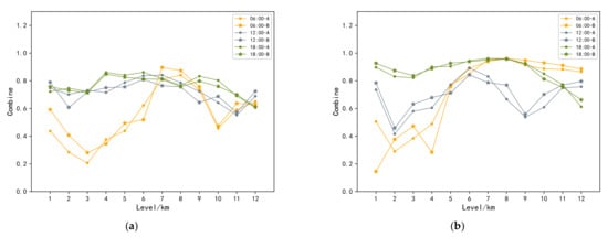
Figure 9.
(a) Line chart of Combine index change of wind speed in each period; (b) line chart of Combine index change of wind direction in each period.

Table 4.
Error comparison of different altitudes.
The results show that the wind speed was above 50% in most periods and more than 70% in most periods. The results have a strong correlation. The correlation of a small part of periods was less than 50%, and the retrieved effect was not ideal. Most of the of the wind direction was above 70%, and the retrieved effect was good, while a small part was below 50%, and the result was slightly worse. Further analysis shows that the lower period basically appears at 06:00 for the same reason as above. Due to the data points being relatively few and the results poor. According to the results of each period, the accuracy of the medium-height layer was relatively stable, which was generally higher than that of other layers. However, the stability of the low altitude was relatively low, which was mainly affected by the amount of data.
5. Optimization of Wind Field Results
The MP model is actually a particle model proposed to study the performance of aircraft. If it is to be applied to meteorology and aviation meteorology, the model needs to be adjusted. In order to strengthen aerial target surveillance, increase airspace flow, apply the retrieved wind field to air traffic control and early warning, and fill the gap of wind field detection data in high altitude, more precise and complete wind field information is needed. However, the wind field obtained by the MP model is still missing in some areas. In view of the above problems, this paper puts forward the following improvement methods.
5.1. Optimization of Meteo-Particle Model Parameter
In this paper, combined with the characteristics of the high-altitude wind field and meteorological knowledge [31], some empirical constant parameters and control factors of the MP model were adjusted to obtain a more real and accurate retrieval of the wind field. ADS-B and Mode S retrieval data and ECMWF ERA5 data were randomly sampled. Each kind of data was randomly divided into 60% and 40%, of which 60% was used as the test data for model parameter optimization, and the experiment was carried out independently. The wind field was retrieved from 60% of the test set data through the MP model, and then the retrieved results were compared with 40% of the original randomly sampled real data. Finally, the accuracy comparison was obtained by calculating the relevant indicators, thus as to optimize the model. In order to reduce the random influence of random walk bias, the mean value of 1000 runs was used to balance the random error, which makes the results more referential and avoids accidental deviation. The influence factors of the main research are shown in Table 5. Through a large number of experiments, the ideal reference values of the factors affecting the retrieval accuracy of the high-altitude wind field and the relevant differences before and after the improvement were obtained. Because the calculated results of each component are similar, only the comparative results of vertical wind components are listed in this paper.

Table 5.
Main influencing factors.
The values of the evaluation indicators are shown in Table 6. Compared with the results of the original model, the indexes of the improved model were significantly optimized. The observation results show that the optimized algorithm greatly improved the accuracy of the 00:00 period. In fact, the optimization model reduced the sensitivity to the amount of data and broadened the scope of application.

Table 6.
Comparison of the accuracy of indexes.
5.2. Continuity of Wind Field
According to the distribution of the ADS-B and Mode S datasets in different periods and different heights, and the lack of wind observation data at low altitudes or at 00:00~06:00, the incompleteness of the wind field was not conducive to its further application. In this paper, the missing data in the retrieved results were analyzed, and the scattered data with irregular intervals needed to be extrapolated. Therefore, a method to reduce the discontinuous wind field was proposed, and the extrapolation method based on Delaunay triangulation was used to obtain more abundant data [32].
The grid wind information retrieved from 4.1 can be expressed as and , and the two components are extrapolated respectively. Firstly, all the information points on the and planes are triangulated to form an edge continuous piecewise triangular surface with point as a node. Then, the triangle to which the extrapolating points belong are found and linear extrapolation is applied within each triangle. Let the points , and be three vertices of an arbitrary triangle on the and planes. The of any point in the triangle can be derived by the following two methods [33,34].
The first method is the binary linear extrapolation given by Equation (20). The linear Equation (21) are obtained by inserting , , and into the equation. Solve the system to obtain the coefficients , , and , and then the rest of the information on the plane can be obtained by calculation.
The second method is obtained by barycentric extrapolation. The position of any point can be uniquely represented as the weighted average value of the three vertex positions shown in the Equation (22) and the , shown in Equation (23), where the weights , , and refer to the coordinates of the barycenter point , which can be obtained by solving the system of Equation (22).
Although the results obtained by the two methods [35] were different in form, in fact, the linear extrapolation results obtained by the two methods were actually the same because the binary linear polynomials passing through the three different given points in space were unique. In this paper, the extrapolation experiment was carried out by using the data at 18:00. Figure 3 is the retrieval of wind field from 17:59:10 to 18:00:50. Compared with the ECMWF ERA5 wind field map at 18:00:00 in Figure 4, there is a serious lack of data in the retrieved wind field data. In order to solve this problem, the extrapolation experiment was carried out by using the above method, and the experimental results are shown in Figure 10. The algorithm completely retains the outline of the retrieval wind field and fills the missing parts of the data. However, considering the shortcomings of the extrapolation method, incorrect estimates may be obtained, and the reliability of the extrapolation results is not as reliable as the retrieval results. Therefore, in the results shown in Figure 10, the retrieval results are represented by black arrows, and the extrapolation results are represented by gray arrows, representing the difference in credibility between the two. In addition, this paper also compares the extrapolation results of each period with ERA5 data. Table 7 and Table 8 are the corresponding verification indicators for each period, and the effect is not bad for this experimental data set. It is similar to the results before extrapolation and does not reduce the accuracy of the results, thus the extrapolation results have a certain reference value.
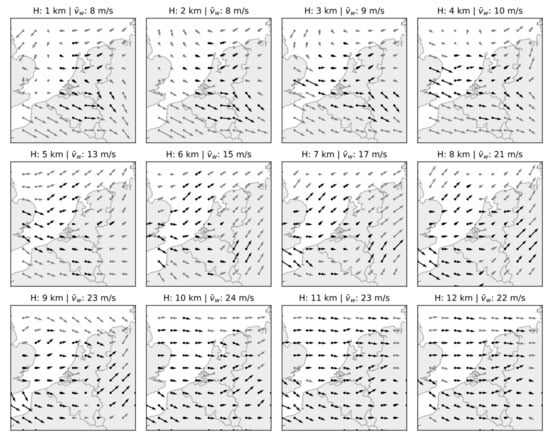
Figure 10.
Extrapolation of the retrieval of wind field from 17:59:10 to 18:00:50 (the black arrow represents the retrieved wind field from the MP model, and the gray arrow represents the extrapolated estimate).

Table 7.
Comparison of u and v errors in different time periods.

Table 8.
Comparison of wind speed and direction errors in different time periods.
It is found that the linear extrapolation method has great limitations and is only suitable for relatively uniform wind fields. It just so happens that the wind field of the Netherlands selected in this paper is a relatively uniform westerly wind, thus the extrapolation result is better. Although the application of the model is based on the exclusion of extreme wind conditions (aircraft avoid extreme atmospheric conditions as far as possible), the application of the extrapolation method is harsh, thus it is not a good method. When we change the dataset with a lot of changes in the wind field, we find that the extrapolation result becomes so bad that it is difficult to apply to other situations. In future work, this paper considers more advanced weather assimilation methods such as 4DVAR to optimize the results.
6. Results and Discussion
At present, the main detection methods of aerial wind fields still rely on sounding balloons, radiosondes, and anemometers. However, the coverage of wind field data obtained by these methods is relatively sparse and cannot meet the research needs of mesoscale meteorology and aeronautical meteorology. In order to further improve the data of the wind field in the high-altitude area, this paper further studies the improved algorithm of the MP model to obtain a wind field with higher accuracy and wider coverage on the basis of the research of JunziSun. In this paper, an evaluation scheme is proposed, which is conducive to the improvement of accuracy and the improvement of the model. It can evaluate the accuracy of the horizontal component, vertical component, wind speed, and wind direction of the retrieval results. Before the improvement of the model, in order to master the characteristics and applicability of the model, the differences of the MP model in different periods and different heights are compared and analyzed. The results show that the MAE value of wind speed is within [1,8], and the MAE value of wind direction is within [4,14]. The accuracy of wind speed is obviously better than that of wind direction. Moreover, among the four periods, 18:00 is the most stable. The main factor affecting the performance of the model is the amount of data, which shows that the model has certain requirements for the amount of data. In addition, the main contribution of this paper is to optimize the model and find a more suitable model parameter value of the meteorological model. Compared with the original model, the optimization model improves the accuracy of the model to some extent. Different wind fields are selected as the experimental data, and the article presents the average value of multiple experimental results of multiple data sets, thus it has high reliability. However, the limitation of this paper is that it is still unable to break the assumptions of the original model. According to the distribution of the retrieval results, the integrity of the wind field is studied at the expense of some accuracy, which makes up for the lack of data and achieves ideal results. It has to be explained here that the linear extrapolation method has uncertainty and has a certain probability of getting incorrect wind information, which can only be used as a reference for weather conditions when there is no data available. Therefore, this paper also distinguishes the retrieval results from the extrapolation results in the experimental results and emphasizes the difference in reliability between them. Compared with the current weather forecast numerical model ECMWF ERA5 data, the retrieval wind field in this paper has higher accuracy and can reflect the useful details that did not exist before. The high-precision wind field obtained by model optimization not only provides a reference for the research of high-altitude wind fields in the meteorological field but also helps to improve air traffic management. In the future, the research will focus on the parameter optimization of the model and the adaptability in the meteorological field. How to make the model parameters have a wide range of adaptability is still the focus of future research. The linear extrapolation method should also be improved, and more advanced weather assimilation methods such as 4DVAR used by ECWMF should be considered.
7. Conclusions
In this paper, the ADS-B and Mode S data obtained from aircraft sensors are used to retrieve the high-altitude wind field by using the MP particle model proposed by Junzi Sun et al., The accuracy and precision of the retrieved results are studied, and the model improvement suggestions and result optimization methods are put forward, which has important reference significance. Current research shows that the coverage of the retrieved wind field is incomplete, and the filtering is usually carried out on the premise of large local accuracy. After the introduction of aircraft data, it is of great importance to contribute to improving the accuracy of the high-altitude wind field. In this paper, a mixed verification index is proposed, which can more effectively evaluate the comprehensive difference of inversion results in wind speed and wind direction. This index can measure the deviation of two vectors in direction and distance at the same time, which makes the measurement of the result more scientific and reasonable. This is not only conducive to the evaluation of the performance of the model but also can be applied to other fields. The most important thing is that the improvement of the parameters of the model improves the accuracy of the retrieval results to a certain extent, and the wind field extrapolation fills the gap of aviation meteorological in the off-route area. The average deviation and correlation of the data obtained by the original algorithm are as follows: component: 3.79 m/s, 82.75%; component: 5.23 m/s, 69.25%; wind speed: 4.68 m/s, 82.50%; wind direction: 7.86 m/s, 77.75%. After improvement and optimization, the average deviation and correlation of the data results in each period are as follows: component: 3.73 m/s, 81.75%; component: 5.37 m/s, 73.21%; wind speed: 4.22 m/s, 82.35%; wind direction: 8.41 m/s, 78%. Although there is no obvious difference in the numerical value of each index of the improved result, in fact, the improved result is overall. On the one hand, the improvement of wind field accuracy makes the retrieval results more detailed, but this optimization cannot be reflected by comparing with ERA5 data. Because reanalyzed datasets such as ERA5 are usually smooth and often have no local changes. Therefore, it is possible that the fine results will reflect a larger error with ERA5, which to some extent neutralizes the advantages of the improved algorithm. On the other hand, the extrapolation algorithm will generally lead to large errors, which will also neutralize the advantages of the improved algorithm to a certain extent. This model can roughly reflect the outline of the wind field and can be used as a reference in the absence of real data. In addition, this paper also makes a comparative analysis of the retrieval of different periods and different altitudes, which provides some reference for other scholars to study the model. For the wind speed, the stability of the results at the lower layer is better than that at the upper layer, and the main influencing factor is the size of the data set. MP model is suitable for the situation with a large number of observations. When the amount of data are small, it will lead to low accuracy. Finally, the expansion of the retrieved wind field is studied, which improves the overall stability of the retrieved wind field on the premise of ensuring the accuracy of the wind field.
Author Contributions
Conceptualization, J.Z.; investigation, J.Z., H.W., J.L. and Z.X.; software, J.Z.; resources, J.Z. and Z.X.; experiment, J.Z. writing of the original draft, J.Z. editing, H.W., J.L. and Z.X.; validation, J.Z.; data analysis, J.Z. and H.W.; review and editing, H.W., J.L. and Z.X.; supervision, H.W.; methodology, J.Z.; formal analysis, H.W. and Z.X. All authors have read and agreed to the published version of the manuscript.
Funding
This research was funded by the National Natural Science Foundation of China (award number U1733103), the Security Ability Fund Program of Civil Aviation Administration of China (ASSA20210061).
Data Availability Statement
The ADS-B raw data used in this study can be found in the OpenSky Network: http://www.opensky-network.org, 16 November 2020, and other data are from the source data used for the experiments of the paper titled “Weather field reconstruction using aircraft surveillance data and a novel meteo-particle model”: https://doi.org/10.6084/m9.figshare.6970403.v1, 20 November 2020. All the data used in this study can be obtained from references given in the text.
Acknowledgments
Results presented in this work have been produced basing on Junzi Sun’s research. The data used in this study was provided by the OpenSky Network, for which we thank them. In addition, the authors would also like to acknowledge the professor Junzi Sun for the provision of data.
Conflicts of Interest
The authors declare no conflict of interest.
References
- Petersen, R.A. On the impact and benefits of AMDAR observations in operational forecasting—Part I: A review of the impact of automated aircraft wind and temperature reports. Bull. Am. Meteorol. Soc. 2016, 97, 585–602. [Google Scholar] [CrossRef]
- Prevot, T.; Homola, J.R.; Martin, L.H.; Mercer, J.S.; Cabrall, C.C. Automated air traffic control operations with weather and time-constraints: A first look at (simulated) far-term control room operations. In Proceedings of the Ninth USA/EUROPE Air Traffic Management Research & Development, Berlin, Germany, 14–17 June 2011. [Google Scholar]
- Banta, R.M.; Pichugina, Y.L.; Kelley, N.D.; Jonkman, B.; Brewer, W.A. Doppler lidar measurements of the Great Plains low-level jet: Applications to wind energy. In IOP Conference Series: Earth and Environmental Science; IOP Publishing: Bristol, UK, 2008. [Google Scholar]
- Shikhovtsev, A.Y.; Kiselev, A.V.; Kovadlo, P.G.; Kolobov, D.Y.; Lukin, V.P.; Tomin, V.E. Method for Estimating the Altitudes of Atmospheric Layers with Strong Turbulence. Atmos. Ocean. Opt. 2020, 33, 295–301. [Google Scholar] [CrossRef]
- Wang, H. ADS-B Used in Improvement of Air Traffic Control. Master’s Thesis, Purdue University, West Lafayette, IN, USA, 2015. [Google Scholar]
- Kun, J.I.A. Data processing of secondary surveillance radar for air traffic control. Telecommun. Eng. 2011, 51, 78–81. [Google Scholar]
- Svyd, I.; Obod, I.; Maltsev, O.; Shtykh, I.; Maistrenko, G.; Zavolodko, G. Comparative quality analysis of the air objects detection by the secondary surveillance radar. In Proceedings of the 2019 IEEE 39th International Conference on Electronics and Nanotechnology (ELNANO), Kyiv, Ukraine, 16–18 April 2019; pp. 724–727. [Google Scholar]
- Galati, G.; Leonardi, M.; Magarò, P.; Paciucci, V. Wide area surveillance using SSR mode S multilateration: Advantages and limitations. In Proceedings of the European Radar Conference, Paris, France, 6 October 2005; pp. 225–229. [Google Scholar]
- Stone, E.K.; Pearce, G. A network of Mode-S receivers for routine acquisition of aircraft-derived meteorological data. J. Atmos. Ocean. Technol. 2016, 33, 757–768. [Google Scholar] [CrossRef]
- Strajnar, B. Validation of Mode-S meteorological routine air report aircraft observations. J. Geophys. Res. Atmos. 2012, 117, D23. [Google Scholar] [CrossRef]
- Mariano, P.; De Marco, P.; Giacomini, C. Data integrity augmentation by ADS-B SSR hybrid techniques. In Proceedings of the 2018 Integrated Communications, Navigation, Surveillance Conference (ICNS), Herndon, VA, USA, 10–12 April 2018; pp. 1–10. [Google Scholar]
- Kulesa, G. Weather and aviation: How does weather affect the safety and operations of airports and aviation, and how does FAA work to manage weather-related effects? In Potential Impacts of Climate Change on Transportation: Workshop Summary and Proceedings, Proceedings of the The Potential Impacts of Climate Change on Transportation, Washington, DC, USA, 1–2 October 2002; US Department of Transportation Center for Climate Change and Environmental Forecasting; US Global Change Research Program; Department of Energy, U.S. Environmental Protection Agency: Washington, DC, USA, 2002. [Google Scholar]
- Bowyer, P.; Hänsel, S.; Smalley, E.; Velegrakis, A.; Dagan, M.; Wyrowski, L. Climate Change Impacts and Adaptation for Transport Networks and Nodes; United Nations Economic Commission for Europe (UNECE): Geneva, Switzerland, 2020. [Google Scholar]
- Kim, E.; Sivits, K. Blended secondary surveillance radar solutions to improve air traffic surveillance. Aerosp. Sci. Technol. 2015, 45, 203–208. [Google Scholar] [CrossRef]
- Sun, J.; Vû, H.; Ellerbroek, J.; Hoekstra, J. Ground-based wind field construction from mode-s and ads-b data with a novel gas particle model. In Proceedings of the Seventh SESAR Innovation Days, Belgrade, Serbia, 27–30 November 2017. [Google Scholar]
- Sun, J.; Vû, H.; Ellerbroek, J.; Hoekstra, J. Weather field reconstruction using aircraft surveillance data and a novel meteo-particle model. PLoS ONE 2018, 13, e0205029. [Google Scholar] [CrossRef] [PubMed]
- De Haan, S.; de Haij, M.; Sondij, J. The Use of a Commercial ADS-B Receiver to Derive Upper Air Wind and Temperature Observations from MODE-S EHS Information in The Netherlands; KNMI: De Bilt, The Netherlands, 2013. [Google Scholar]
- Schäfer, M.; Strohmeicr, M.; Smith, M.; Lenders, V.; Martinovic, I. OpenSky report 2018: Assessing the integrity of crowdsourced mode S and ADS-B data. In Proceedings of the 2018 IEEE/AIAA 37th Digital Avionics Systems Conference (DASC), London, UK, 23–27 September 2018; pp. 1–9. [Google Scholar]
- Schäfer, M.; Strohmeier, M.; Lenders, V.; Martinovic, I.; Wilhelm, M. Bringing up OpenSky: A large-scale ADS-B sensor network for research. In Proceedings of the IPSN-14 Proceedings of the 13th International Symposium on Information Processing in Sensor Networks; Berlin, Germany, 15–17 April 2014, pp. 83–94.
- Bolbasova, L.A.; Shikhovtsev, A.Y.; Kopylov, E.A.; Selin, A.A.; Lukin, V.P.; Kovadlo, P.G. Daytime optical turbulence and wind speed distributions at the Baikal Astrophysical Observatory. Mon. Not. R. Astron. Soc. 2019, 482, 2619–2626. [Google Scholar] [CrossRef]
- Sun, J.; Vû, H.; Ellerbroek, J.; Hoekstra, J.M. Pymodes: Decoding mode-s surveillance data for open air transportation research. IEEE Trans. Intell. Transp Syst. 2019, 21, 2777–2786. [Google Scholar] [CrossRef]
- Huy, V. ADS-B and Mode S Data for Aviation Meteorology and Aircraft Performance Modelling. Mater’s Thesis, Delft University of Technology, Delft, The Netherlands, 2018. [Google Scholar]
- Trüb, R.; Moser, D.; Schäfer, M.; Pinheiro, R.; Lenders, V. Monitoring meteorological parameters with crowdsourced air traffic control data. In Proceedings of the 2018 17th ACM/IEEE International Conference on Information Processing in Sensor Networks (IPSN), Porto, Portugal, 11–13 April 2018; pp. 25–36. [Google Scholar]
- Delahaye, D.; Puechmorel, S. TAS and wind estimation from radar data. In Proceedings of the 2009 IEEE/AIAA 28th Digital Avionics Systems Conference, Orlando, FL, USA, 23–29 October 2019; p. 2B. [Google Scholar]
- Hrastovec, M.; Solina, F. Obtaining meteorological data from aircraft with Mode-S radars. IEEE Aerosp. Electron. Syst. Mag. 2013, 28, 12–24. [Google Scholar] [CrossRef]
- Lu, M.; Qin, Z.; Cao, Y.; Liu, Z.; Wang, M. Scalable news recommendation using multi-dimensional similarity and Jaccard–Kmeans clustering. J. Syst. Softw. 2014, 95, 242–251. [Google Scholar] [CrossRef]
- Liu, F.; Guo, W. Multi-dimensional Similarity Personalized Recommendation Model in Deep Learning Mode. In Data Processing Techniques and Applications for Cyber-Physical Systems (DPTA 2019); Springer: Singapore, 2020; pp. 689–698. [Google Scholar]
- Ming, D. Community Detection Algorithm Based on Similarity Index. Master’s Thesis, Shandong Normal University, Jinan, China, 2018. [Google Scholar]
- De Haan, S.; Stoffelen, A. Assimilation of high-resolution Mode-S wind and temperature observations in a regional NWP model for nowcasting applications. Weather Forecast. 2012, 27, 918–937. [Google Scholar] [CrossRef]
- De Haan, S. High-resolution wind and temperature observations from aircraft tracked by Mode-S air traffic control radar. J. Geophys. Res. Atmos. 2011, 116, D10. [Google Scholar] [CrossRef]
- Gultepe, I.; Sharman, R.; Williams, P.D.; Zhou, B.; Ellrod, G.; Minnis, P.; Trier, S.; Griffin, S.; Yum, S.S.; Gharabaghi, B.; et al. A review of high impact weather for aviation meteorology. Pure Appl. Geophys. 2019, 176, 1869–1921. [Google Scholar] [CrossRef]
- Stead, S.E. Estimation of gradients from scattered data. Rocky Mt. J. Math. 1984, 14, 265–279. [Google Scholar] [CrossRef]
- Amidror, I. Scattered data interpolation methods for electronic imaging systems: A survey. J. Electron. Imaging 2002, 11, 157–176. [Google Scholar] [CrossRef]
- De Berg, M.; Cheong, O.; van Kreveld, M.; Overmars, M. Delaunay triangulations: Height interpolation. In Computational Geometry: Algorithms and Applications; Springer: Berlin, Germany, 2008; Chapter 9; pp. 191–218. [Google Scholar]
- Nielson, G.M. Tools for Triangulations and Tetrahedrizations. In Scientific Visualization; Springer: Berlin, Germany, 1997; Chapter 20; pp. 429–525. [Google Scholar]
Publisher’s Note: MDPI stays neutral with regard to jurisdictional claims in published maps and institutional affiliations. |
© 2021 by the authors. Licensee MDPI, Basel, Switzerland. This article is an open access article distributed under the terms and conditions of the Creative Commons Attribution (CC BY) license (https://creativecommons.org/licenses/by/4.0/).