Train Performance Analysis Using Heterogeneous Statistical Models

Abstract

This study investigated the effect of a harsh winter climate on the performance of high-speed passenger trains in northern Sweden. Novel approaches based on heterogeneous statistical models were introduced to analyse the train performance to take time-varying risks of train delays into consideration. Specifically, the stratified Cox model and heterogeneous Markov chain model were used to model primary delays and arrival delays, respectively. Our results showed that weather variables including temperature, humidity, snow depth, and ice/snow precipitation have a significant impact on train performance.

1. Introduction

Coldness, heavy snow and ice/snow precipitation are well-known winter phenomena in the northern region of Sweden. Such a climate can cause severe problems to railway transportation as well as the people who rely on it, which leads to ineluctable impacts on the normal operation of the whole society. It has become an especially prominent problem recently, as the railway network has become more complicated, the trains run faster, and more people choose rail as their travel mode. The aim of this study is thus to analyse the harsh winter effects on railway operation in northern Sweden. Regarding railway operation, punctuality is one key criteria to minimise societal costs and increase the reliability of railway operation. Therefore, the aim of the study is to investigate and figure out how train delays are affected by the winter climate.

Primary delay and arrival delay are two commonly used measurements in train operation. Primary delay measures the increment in delay within two consecutive measuring spots in terms of running time, and arrival delay is the delay in terms of arrival time at a measuring spot. The time limits to define primary delays and arrival delays vary from country to country [1]. According to the Swedish Transport Administration (STA), a train arriving at one measuring spot within five minutes is not considered to be arrival delay, and a delay of three minutes or more in terms of running time within two consecutive measuring spots is considered to be primary delay. One of the main interests from the STA is to investigate how the two kinds of train delays are affected by winter weather. Therefore, we apply the STA criteria throughout the study.

Several studies of train performance analysis have been conducted. Yuan [1] used probability models based on blocking time theory to estimate the knock-on delays of trains caused by route conflicts and late transfer connections in stations. In Murali et al. [2], the authors modelled travel-time delay as a function of the train mix and the network topology. Lessan et al. [3] proposed a hybrid Bayesian network model to predict arrival and departure delays in China. Huang et al. [4] pointed out in their paper that arrival delay was highly correlated with capacity use of the train line. In a more recent study, Huang et al. [5] applied a Bayesian network to predict disruptions and disturbances during train operations in China. In addition to those, a few earlier studies of the relationships between train performance and weather have also been investigated. Thornes and Davis [6] investigated the effects of temperature, snow, ice, humidity and other weather variables on railway delays in the UK. Four case studies in Ludvigsen and Klboe [7] showed that harsh winter weather in 2010, for example low temperatures, heavy snowfall and strong winds, affected freight train delays in Norway, Sweden, Switzerland and Poland. Xia et al. [8] fitted a linear model and showed that weather variables such as snow, temperature, precipitation and wind had significant effects on the punctuality of trains in the Netherlands. The effect of snowfall and rainfall in winter on delays of passenger trains in Hungary was identified in Nagy and Csiszár [9]. Brazil et al. [10] used a simple multiple linear regression model and demonstrated that weather variables, such as wind speed and rainfall, can have a significantly negative impact on arrival delays in the Dublin-area rapid-transit rail system. A machine-learning approach was used to create a predictive model to predict the arrival delay at each station for a train line in China with the help of weather observations in Wang and Zhang [11]. Ottosson [12] used negative binomial regression and a zero-inflated model and showed that weather variables, such as snow depth, temperature and wind direction, had significant effects on the train performance. A recent study by Wang et al. [13] applied a non-stratified Cox model and homogeneous Markov chain model to analyse the weather effects on primary delay and arrival delay, respectively. The authors treated primary delay as recurrent time-to-event data, and the transitions between states (arrival) delay and punctuality in a train trip as a Markov chain. One limitation was that the hazard function in the Cox model was assumed to be constant over events, and the transition intensity in the Markov chain model cannot change at any specified time. However, these assumptions are often not realistic.

In this study, we relax the restrictions in Wang et al. [13] by assuming heterogeneity in the models, i.e., hazard functions vary among events, and transition intensity may change at any specified time point. The main contribution is that we prove that the heterogeneous models outperform the homogeneous counterparts. In addition, to the best of our knowledge, this is the first study to apply heterogeneous models to investigate the weather impacts on the train-delay issues, i.e., a stratified Cox model is used to investigate how winter climate affects the occurrence of primary delays, and a heterogeneous Markov chain model is applied to study the effect of winter climate on the transitions between delayed and punctual states.

The paper is organized as follows. In Section 2, we introduce the statistical models in detail. Data processing and analysis methods are described in Section 3. Section 4 is reserved for results. Section 5 is devoted to the conclusion and discussion.

2. Statistical Modelling

In this section, the two statistical models, i.e., stratified Cox model and heterogeneous Markov chain model, are introduced in detail.

2.1. Stratified Cox Model with Time-Dependent Covariates for Recurrent Event

As an extension of original Cox models in Cox [14], Andersen and Gill [15], Prentice et al. [16] proposed a stratified Cox model, which is commonly used for modelling recurrent events in survival analysis. It will be used in this study to analyse the relationship between hazards of trains with recurrent events (primary delay) and weather covariates by assuming that the hazard function of a train is correlated with its preceding events through an event-specific baseline hazard function. Formally, the stratified Cox model with time-dependent covariates for recurrent events is an expression of the hazard function and covariates

$$h_{ij}\left(t\right)=h_{0j}\left(t\right)\text{exp}\left({\beta }^T{x}_{ij}\left(t\right)\right),$$

(1)

where

• $h_{ij}\left(t\right)$ represents the hazard function for the jth event of the ith train at time t.
• $h_{0j}\left(t\right)$ is an event-specific baseline hazard and the order number j is the stratification variable, e.g., $h_{01}\left(t\right)$ is a common baseline hazard of the first event for each train.
• $x_{ij}\left(t\right)$ represents the weather covariate vector for the ith train and the jth event at time t.
• $\beta$ is an unknown coefficient vector to be estimated, the exponential of which indicates how the hazard ratios are affected by the covariate vector.

The coefficients can be estimated by maximising the partial likelihood, given by

$$L\left(\beta \right)=\prod _{i=1}^n\prod _{j=1}^{k_i}{\left(\frac{\text{exp}\left({\beta }^T{x}_i\left(t_{ij}\right)\right))}{{\sum }_{l\in R\left(t_{ij}\right)}\text{exp}({\beta }^T{x}_l\left(t_{ij}\right))}\right)}^{{\delta }_{ij}},$$

(2)

where j is the event index with $k_i$ being the train-specific maximum number of events, $x_i\left(t_{ij}\right)$ denotes the covariate vector for the ith train at the jth event time $t_{ij},$${\delta }_{ij}$ is an event indicator that equals 1 for the jth event of the ith train and 0 for censoring, $R\left(t_{ij}\right)=\{l,l=1,\cdots ,n:t_{l(j-1)}<t_{ij}\le t_{lj}\}$ is a group of trains that is at risk of the jth event at time $t_{ij}$. Please note that the partial likelihood takes into account the conditional probabilities for the events that occur for trains.

The fitted model can then be used to predict the hazard function, ${\widehat{h}}_{ij}\left(t\right)$, for the jth event of train i of interest given the values of covariates, as well as corresponding survival function, ${\widehat{S}}_{ij}\left(t\right)$, which gives the probability that the train i does not suffer the jth event up to time t. The survival function is an exponential function of the hazards function, i.e., ${\widehat{S}}_{ij}\left(t\right)=\text{exp}\left(-{\int }_0^t{\widehat{h}}_{ij}\left(x\right)\mathrm{d}x\right)$.

2.2. Heterogeneous Markov Chain Model with Time-Dependent Covariates

Let $\left\{Y\right(t),t\ge 0\}$ denote a continuous time Markov chain. At each time point t, $Y\left(t\right)$ takes a value over a countable state space. The probability of chain $Y\left(t\right)$ being in state s at time t is $P\left(Y\right(t)=s)$. The conditional probability $p_{rs}(t,t+u)=P(Y(t+u)=s|Y\left(t\right)=r)$ represents the transition probability of moving from the state r at time t to the state s at time $t+u$. The instantaneous movement from state r to state s at time t is governed by transition intensity, $q_{rs}\left(t\right)$, through the transition probabilities

$$q_{rs}\left(t\right)=\underset{\Delta t\to 0}{\text{lim}}P(Y(t+\Delta t)=s|Y\left(t\right)=r)/\Delta t.$$

(3)

With these definitions, a Markov chain can be used to describe train running states (delay/punctuality) on a train line, where the time t refers to running distance of a train from the starting point throughout the study instead of time, since the running distance is more meaningful in practice. The $q_{rs}\left(t\right)$ of a q states process forms a $q\times q$ transition intensity matrix $Q\left(t\right)$, whose rows sum to zero, so that the diagonal entries are defined by $q_{rr}\left(t\right)=-{\sum }_{s\ne r}{q}_{rs}\left(t\right)$. An example of transition intensity matrix $Q\left(t\right)$ with two states can be seen below

$$Q\left(t\right)=\left[\begin{array}{cc}{q}_{11}\left(t\right)& q_{12}\left(t\right)\\ q_{21}\left(t\right)& q_{22}\left(t\right)\end{array}\right],$$

(4)

where $q_{11}\left(t\right)=-q_{12}\left(t\right)$ and $q_{22}\left(t\right)=-q_{21}\left(t\right)$ at time t.

A homogeneous Markov chain in time means that the transition intensity $Q\left(t\right)$ is independent of t, and the transition probability from one state to another depends solely on the time difference between two time points, i.e.,

$$P\left(Y\right(t+u)=s|Y\left(t\right)=r)=P(Y\left(u\right)=s\left|Y\right(0)=r).$$

(5)

Corresponding to the transition intensity matrix Q, the entry in a transition probability matrix $P(t,t+u)$ is the transition probability $p_{rs}(t,t+u)$. The relationship between transition intensity matrix and transition probability matrix is specified through the Kolmogorov differential equations [17]. In particular, when a process is homogeneous, the transition probability matrix can be calculated by taking the matrix exponential of the transition intensity matrix

$$P(t,t+u)=P\left(u\right)=\mathrm{Exp}\left(uQ\right).$$

(6)

In a homogeneous Markov chain model, to take account of the effect of covariates, a Cox-like model was proposed by Marshall and Jones [18]

$$q_{rs}=q_{rs}^{\left(0\right)}\text{exp}\left({\beta }_{rs}^T{x}_{rs}\right),$$

(7)

where $q_{rs}^{\left(0\right)}$ is a baseline transition intensity from state r to state s when all covariates are zero and $x_{rs}$ is a covariate vector under the corresponding transition. The value $\text{exp}\left({\beta }_{rs}\right)$, where ${\beta }_{rs}$ is one element of the vector ${\beta }_{rs},$ reflects how the corresponding covariate affects the hazard ratio given that all other covariates are held constant. More specifically, $\text{exp}\left({\beta }_{rs}\right)>1$ indicates the transition intensity from r to s increases as the value of the covariate increases, $\text{exp}\left({\beta }_{rs}\right)<1$ indicates the transition intensity decreases as the value of the covariate increases, while $\text{exp}\left({\beta }_{rs}\right)=1$ implies the covariate has no effect on the transition intensity.

The coefficient vectors ${\beta }_{rs}$ as well as the transition intensity matrix Q and the transition probability matrix $P\left(t\right)$ can be estimated by maximising the likelihood

$$L\left(Q\right)=\prod _{i=1}^n\prod _{j=1}^{c_i}{p}_{Y\left(t_{i,j}\right),Y\left(t_{i,j+1}\right)}(t_{i,j+1}-t_{i,j}),$$

(8)

where j is a sequence index of observed states with $c_i$ being number of measuring spots for train i on the train line, $Y\left(t_{i,j}\right)$ represents the jth observed state of the ith train at time $t_{i,j}$ and the transition probability is evaluated at the time difference $t_{i,j+1}-t_{i,j}$.

Contrary to the homogeneous Markov chain model, a heterogeneous Markov chain model assumes that the transition intensity may change continuously at any time. However, the transition probability matrix as well as the likelihood (8) are analytically intractable under this situation [19]. An exception is that the transition intensity changes at countable time points. For example, the transition intensity is assumed to change at time point $t_0$ for each train. To achieve it, one can introduce an indicator covariate in the model to represent the two time periods

$$q_{rs}\left(t\right)=q_{rs}^{\left(0\right)}\text{exp}({\beta }_{rs}^T{x}_{rs}^{\left({\mathbb{1}}_{\{t\ge t_0\}}\right)}+z_{rs}{\mathbb{1}}_{\{t\ge t_0\}}),$$

(9)

where $\mathbb{1}$ is an indicator function taking value 1 if $t\ge t_0$, otherwise, 0, and $z_{rs}$ is the coefficient. Please note that the covariate vector under the same transition is separated into two at $t_0$ through the indicator function, since (9) can be formulated as two homogeneous models and each model has its own covariate vector, i.e., $x_{rs}^{\left(0\right)}$ for the first model when $t<t_0$ and $x_{rs}^{\left(1\right)}$ for the second model when $t\ge t_0$. Similar to $\text{exp}\left({\beta }_{rs}\right)$, the value $\text{exp}\left(z_{rs}\right)$ is the hazard ratio of intensities between $t\ge t_0$ and $t<t_0$ for the transition from r to s.

After fitting the heterogeneous Markov chain model, one can calculate the predicted transition probability matrix for any operational interval of interest on the train line using (6) provided that values of covariates for the interval are given.

3. Data and Method

This section describes the train data and weather variables used for the analysis as well as an imputation method for the missing train records. Moreover, a model comparison method, likelihood ratio test, is presented which is used to compare the performance between the heterogeneous models and homogeneous models.

3.1. Train Data

Our investigation focuses on high-speed passenger trains, which is a type of train with a top speed of between 200 and 250 km/h, between Umeå and Stockholm in the northern region. The high-speed passenger train is chosen because this type of train has higher priority on the train line and often travels longer distances, which can minimise non-natural effects on the train line so that it is easier to detect the pure weather impacts. The data window chosen is December 2016–February 2017, which is typical wintertime in Sweden.

A train line comprises of several measuring spots where the operational times are recorded such as departure and arrival times. The train line between Umeå and Stockholm includes 116 measuring spots in total. The total length of the train line is 711 km and the planned drive time for a high-speed passenger train is approximately 6.5 h. The lengths of any two consecutive measuring spots vary from 0.3 km to 15 km. The key variables are listed in

Table 1. List of variables in the train operation data.

Variables	Description
Train Number	An identification number for train used in the trip
Arrival location	Name of arrival measuring spot
Departure location	Name of departure measuring spot
Departure date	The departure date (yyyy-mm-dd) for a train at a location
Arrival date	The arrival date (yyyy-mm-dd) for a train at a location
Train type	Type of train, for example: high-speed, commuter train and regional
Section Length	Length (km) between two consecutive measuring spots
Planned departure time	The planned departure time (hh:mm) at a measuring spot
Planned arrival time	The planned arrival time (hh:mm) at a measuring spot
Actual departure time	The Actual departure time (hh:mm) at a measuring spot
Actual arrival time	The Actual arrival time (hh:mm) at a measuring spot

.

To fit the two statistical models to the train data, the data should be organized to include the following variables, e.g., each record has one departure spot of the train run (it is not necessary in the Markov chain model), its subsequent arrival spot, distances of these two measuring spots from starting station, and indicators of primary delay and arrival delay, 0/1, for this running section, as well as corresponding weather covariates and train identification number. To obtain the indicator variables for primary delay and arrival delay, one needs to calculate the running time difference and arrival time difference compared to the schedule, which are (actual arrival time—actual departure time)—(planned arrival time—planned departure time) and (actual arrival time—planned arrival time), respectively. Afterwards, the values for the two indicator variables can be assigned, i.e., 1 stands for a primary/arrival delay, 0 otherwise. An example of how to derive the indicator variables along a train line is illustrated in Figure 1.

3.2. Weather Data

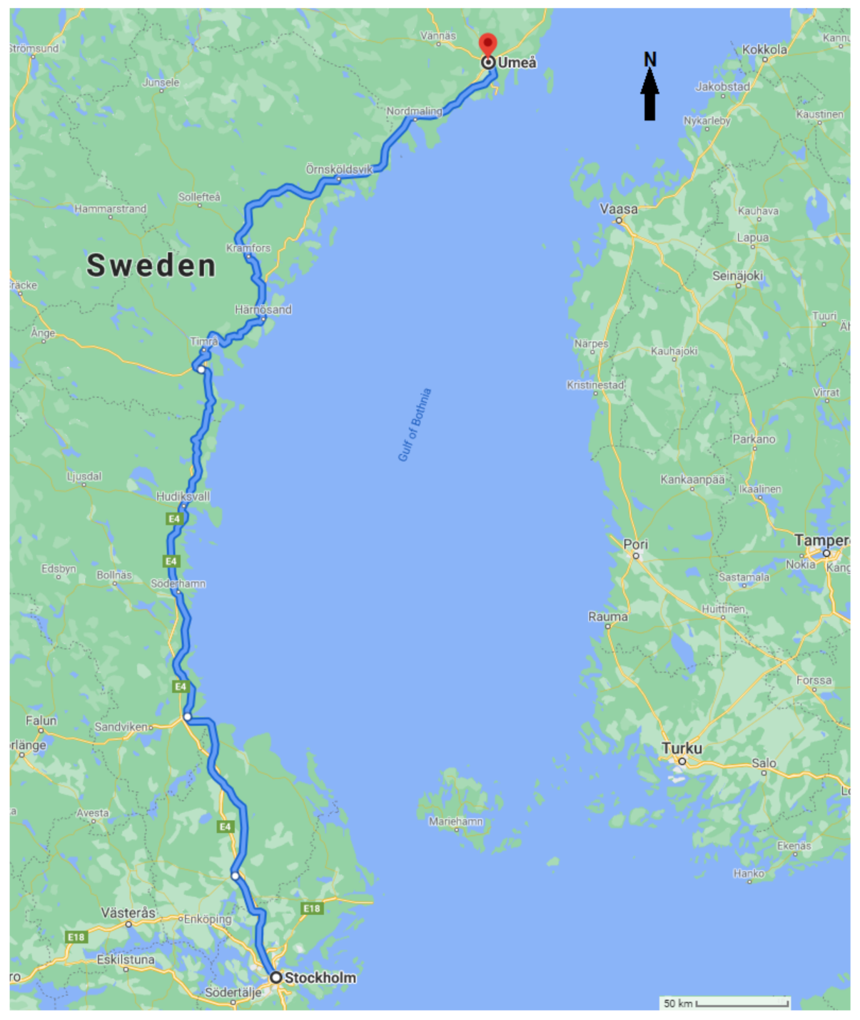
The weather data from December 2016 to February 2017 is simulated from the Weather Research and Forecasting (WRF) model instead of using real meteorological observations, since the distances between the nearest meteorological station and measuring spot along the train line range from 17 to 24 km [12]. Thus, using meteorological data is not an ideal choice in the analysis. However, a WRF model is a numerical weather prediction system that is used for research and operational purposes. Its reliable performance has been assessed in several studies [20,21,22,23]. The WRF model simulates the desired weather variable estimations over grids. Higher spatial resolution implies smaller grids over a region of interest. Temporal resolution decides the time interval between each simulation. Therefore, a WRF with high spatio-temporal resolution is a good alternative under this situation. In this study, the spatial resolution is set as $3\times 3$ km and the temporal resolution is set as 1 h. The simulation region as well as the train line of interest are shown in Figure 2.

The weather variables of interest are shown in

Table 2. The weather variables of interest.

Variables	Description
Temperature	The temperature (${}^{\circ }$C) at 2 m above the ground
Humidity	Relative Humidity (%) at 2-m
Snow depth	The snow depth in centimetres (cm)
Ice/snow precipitation	Hourly accumulated ice/snow in millimetre (mm)

. These variables are chosen because they are believed to have impacts on the train operation in winter and have been used in Ottosson [12], Wang et al. [13].

The measuring time in train operation data must be rounded to the closest hour, so that every measuring spot on the train line can be matched with the closest grid point by date and time.

The average of the weather variables within any two consecutive spots are calculated and used in the analysis. Since a large number of the ice/snow precipitation values are zero along the train line, a categorical variable is used instead of a continuous variable, i.e., 0 if ice/snow precipitation is zero, 1 otherwise.

3.3. Missing Values in the Train Operation Data

A section between two consecutive measuring spots for a train trip often has missing departure/arrival times that can be classified into three different classes, which are defined in

Table 3. Classes of missing times.

Class	Departure Time Missing	Arrival Time Missing
1	True	False
2	False	True
3	True	True

.

A common method to impute missing values in such longitudinal data is called last observation carried forward (LOCF), i.e., the latest recorded value is used to impute the missing value. The advantages of using LOCF are that the number of observations removed from the study decreases and makes it possible to study all subjects over the whole time period. A disadvantage of the method is the introduction of bias of the estimates if the values change considerably with time, or the time period between the most recent value and the missing value is long. Because the intervals with missing values are short in the dataset, which decreases the risk of bias, it is reasonable to apply this approach. Based on the LOCF, the imputation procedure is explained further below.

(1)

Start from the beginning of the trip and save the latest arrival and departure time until a missing time is occurring.

(2)

If the missing time is arrival time, then (a); if departure time is missing then (b):

(a)

Replace the missing arrival time with the latest departure time + the planned driving time for the previous section

(b)

Replace the missing departure time with the latest arrival time + the planned dwell time.

(3)

Save the imputed time as the new latest time.

(4)

If the section is not the last section of the trip, go back to step 1.

3.4. Likelihood Ratio Test

The likelihood ratio test is a hypothesis test that helps to determine whether adding complexity to a simple model makes the complex model significantly better compared to the simple model. Under the study context, comparisons occur between the two (complex) heterogeneous models against the two (simple) homogeneous models, respectively. The likelihood ratio test statistic is given by

$$\lambda =-2ln\left(\frac{{\mathcal{L}}_{homo}\left(\widehat{\theta }\right)}{{\mathcal{L}}_{heter}\left(\widehat{\theta }\right)}\right),$$

(10)

where the numerator in the bracket is the likelihood value for a homogeneous model with estimated parameter vector $\widehat{\theta }$, while the denominator represents the likelihood for the corresponding heterogeneous model. The null hypothesis in the simple model is better and a low p value leads to the rejection of the null hypothesis and favouring of the complex model.

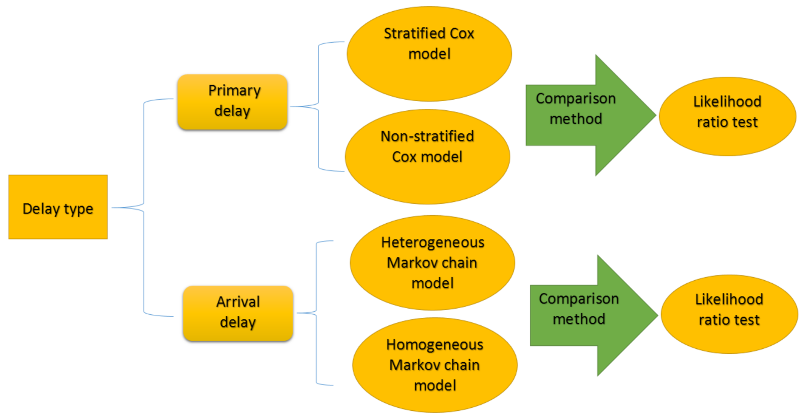
For the purposes of clarity, Figure 3 summarises the related statistical methodologies used for the analysis of the two types of delays as well as the model comparison method, respectively.

3.5. Analysis Tool

R is the software used for data processing and modelling. Specifically, the package survival is used for the stratified Cox model and the package msm is used for the heterogeneous Markov chain model.

4. Results

4.1. Stratified Cox Model

The estimates from the fitted stratified Cox model with 95% confidence intervals (CIs) and p-values can be found in

Table 4. Estimates from the fitted stratified Cox model.

Predictor	Hazard Ratio	CI: Lower	CI: Upper	p-Value
Temperature	0.964	0.933	0.997	0.0338
Humidity	1.017	1.003	1.030	0.0107
Snow depth	1.017	0.990	1.044	0.2197
Ice/snow precipitation	1.055	0.841	1.323	0.6465

. Temperature and humidity are two variables that have significant effects on the occurrence of the primary delay. To be specific, as temperature increases with $1{}^{\circ }$C, the hazard decreases 3.6%, and as humidity increases 1%, the hazard increases 1.7%. Comparison between the stratified Cox model and the non-stratified Cox model in Wang et al. [13] using a likelihood ratio test shows that the stratified model is significantly better than the non-stratified model ($p<0.0001$).

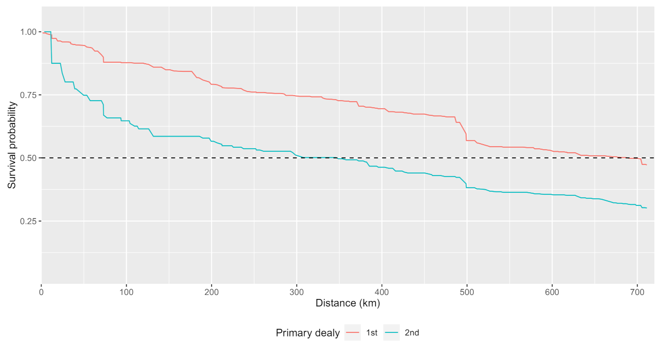
Besides hazard ratios, a survival plot is also produced to show how survival probabilities vary between the first and second occurrence of primary delays in Figure 4. The survival curves for the higher orders of primary delays are not shown due to the data deficiency. The curves are plotted under the condition with the average of temperature, humidity and snow depth among the whole data together with ice/snow precipitation, i.e., temperature is $-1.2{}^{\circ }$C, humidity is 85%, snow depth is 3 cm and ice/snow precipitation is 1.

The figure clearly indicates that slightly less than 50% of trains do not experience any primary delay during the trip, and 50% of trains that have experienced the first primary delay suffer second primary delays after running 330 km from the starting point. It is interesting to note that there is a substantial reduction in survival probability right before running 500 km from the starting point for the first primary delay. The reason for this might be related to some mechanical problems of trains in winter.

4.2. Heterogeneous Markov Chain Model

As indicated in Figure 4, under the average weather conditions, half of the number of the first two primary delays occur in the second part of the trip partitioned at 330 km, thus it is reasonable to assume the transition intensities are different before and after running 330 km. Therefore, $t_0=330$ is chosen when modelling heterogeneous Markov chain (9).

Table 5. Hazard ratios from punctual to delayed states.

Predictor	Hazard Ratio	CI: Lower	CI: Upper	p-Value
Temperature	0.988	0.962	1.015	0.3881
Humidity	0.990	0.980	1.001	0.0683
Snow depth	1.000	0.977	1.026	0.9442
Ice/snow precipitation	1.230	1.001	1.512	0.0489

and

Table 6. Hazard ratios from delayed to punctual states.

Predictor	Hazard Ratio	CI: Lower	CI: Upper	p-Value
Temperature	1.044	1.016	1.073	0.0022
Humidity	0.984	0.973	0.995	0.0036
Snow depth	0.952	0.924	0.980	0.0012
Ice/snow precipitation	0.890	0.719	1.103	0.2921

present the hazard ratios from the heterogeneous Markov chain model with 95% CIs and p-values. The ice/snow precipitation has a significant impact on the transition from punctual to delayed states in Table 5, which means that the transition intensity from punctuality to delay increases 23% with ice/snow precipitation. In contrast, temperature, humidity and snow depth have significant impacts on the transition from delayed to punctual states. It indicates in Table 6 that as the temperature increases 1 ${}^{\circ }$C, the transition intensity from delayed to punctual states increases 4.4%, as the humidity increases 1%, the transition intensity decreases 1.6%, and as the snow depth increases 1 cm, the transition intensity decreases 4.8%. Likelihood ratio test between the heterogeneous Markov chain model (9) and the homogeneous Markov chain model in Wang et al. [13] is also performed, which shows that our new model (9) fits significantly better with $p<0.0001$ than the homogeneous one.

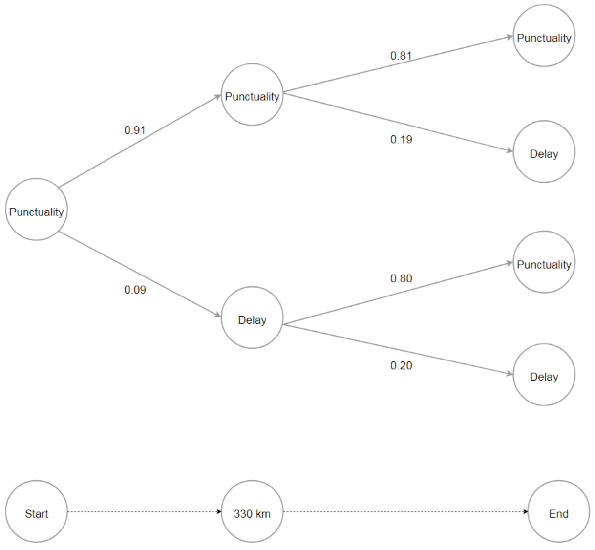
Using the average of temperature, humidity and snow depth together with ice/snow precipitation,

Table 7. Estimated hazard ratios between segments $[330,\mathrm{end})$ and $[0,330)$.

Predictor	Hazard Ratio	CI: Lower	CI: Upper	p-Value
Punctuality—delay	1.586	1.337	1.883	<0.0001
Delay—punctuality	0.681	0.564	0.822	<0.0001

and Figure 5 show the estimated transition intensities and probabilities of evolution of delayed status for the two segments divided at 330 km, respectively. In Table 7, the transition intensity of the second segment of the trip from punctual to delayed states is 58.6% higher than the first; however, transition intensity of the second segment of the trip from delayed to punctual states is 31.9% lower than the first segment. In other words, the second segment is much more likely to suffer delay and more difficult to recover from a delay. It is also verified in Figure 5 that the first segment has a higher probability of being punctual. Since the arrival delay analysis is conducted over all the measuring spots after the starting point, and the state of the train at the initial station is not considered, and for the purpose of illustration of the difference of transition intensities between the two segments shown in Table 7, Figure 5 only presents the trip that begins with a punctual state. Under such an assumption, the probability of a train arriving at the final station on time is about 81% $(0.91\times 0.81+0.09\times 0.80=0.809)$.

5. Discussion

In the study, we considered the heterogeneity within each train in both statistical models; however, the heterogeneity among trains is not touched on yet and could be considered for further investigation, for example a frailty Cox model and/or fitting the two models from a Bayesian perspective with random effects among trains [24]. In addition, choosing the changing point and the number of changing points in a heterogeneous Markov chain process become critical problems, since the estimated transition intensity matrix may be sensitive to the choices, which are very subjective. In this study, only one changing point at 330 km was used, which was decided by the fact that half of the number of the first two primary delays occurred in the second part of the trip partitioned at 330 km under the average weather condition in Figure 4. Continuously changing transition intensities, which are a smooth function of time, e.g., a Weibull-distributed time function, may be more plausible with the help of numerical approximation methods [19]. Moreover, more could be done in terms of statistical modelling. For instance, (1) a more-than-two-states Markov chain model can be used to acquire a deeper understanding of the climate effects; (2) more than one changing point of the transition intensity can be investigated in the model; and (3) interactions between weather variables and the indicator variable could be considered to account for the weather effects in each segment in the heterogeneous Markov chain model. Moreover, train operation data from more than one winter could to be included in the model-fitting procedure to acquire more robust inference.

6. Conclusions

This study investigated the effects of a harsh winter climate on the performance of high-speed passenger trains in northern Sweden, with respect to the occurrence of primary delays and the transition intensities between delayed and punctual states. Novel approaches based on heterogeneous statistical models were introduced to analyse the train performance to take the time-varying risks of train delays into consideration. Specifically, a stratified Cox model and a heterogeneous Markov chain model were used to modelling primary delays and arrival delays, respectively. We conclude that (1) the two heterogeneous models outperform the homogeneous counterparts; (2) the weather variables, including temperature, humidity, snow depth, and ice/snow precipitation, have significant impacts on train delays.

References

1. Yuan, J. Dealing with Stochastic Dependence in the Modeling of Train Delays and Delay Propagation. Ph.D. Thesis, TRAIL Research School, Delft University of Technology, Delft, The Netherlands, 2006. [Google Scholar] [CrossRef]
2. Murali, P.; Dessouky, M.; Ordóñez, F.; Palmer, K. A delay estimation technique for single and double-track railroads. Transp. Res. Part E Logist. Transp. Rev. 2010, 46, 483–495. [Google Scholar] [CrossRef]
3. Lessan, J.; Fu, L.; Wen, C. A hybrid Bayesian network model for predicting delays in train operations. Comput. Ind. Eng. 2019, 127, 1214–1222. [Google Scholar] [CrossRef]
4. Huang, P.; Wen, C.; Li, J.; Peng, Q.; Li, Z.; Fu, Z. Statistical Analysis of Train Delay and Delay Propagation Patterns in a High-Speed Railway System. In Proceedings of the 2019 5th International Conference on Transportation Information and Safety (ICTIS), Liverpool, UK, 14–17 July 2019; pp. 664–669. [Google Scholar] [CrossRef]
5. Huang, P.; Lessan, J.; Wen, C.; Peng, Q.; Fu, L.; Li, L.; Xu, X. A Bayesian network model to predict the effects of interruptions on train operations. Transp. Res. Part C Emerg. Technol. 2020, 114, 338–358. [Google Scholar] [CrossRef]
6. Thornes, J.; Davis, B. Mitigating the impact of weather and climate on railway operations in the UK. In Proceedings of the ASME/IEEE Joint Railroad Conference, Washington, DC, USA, 23–25 April 2002; pp. 29–38. [Google Scholar] [CrossRef]
7. Ludvigsen, J.; Klæboe, R. Extreme weather impacts on freight railways in Europe. Nat. Hazards 2013, 70, 767–787. [Google Scholar] [CrossRef]
8. Xia, Y.; Van Ommeren, J.N.; Rietveld, P.; Verhagen, W. Railway infrastructure disturbances and train operator performance: The role of weather. Transp. Res. Part D Transp. Environ. 2013, 18, 97–102. [Google Scholar] [CrossRef]
9. Nagy, E.; Csiszár, C. Analysis of Delay Causes in Railway Passenger Transportation. Periodica Polytech. Trans. Eng. 2015. [Google Scholar] [CrossRef] [Green Version]
10. Brazil, W.; White, A.; Nogal, M.; Caulfield, B.; O’Connor, A.; Morton, C. Weather and rail delays: Analysis of metropolitan rail in Dublin. J. Transp. Geogr. 2017, 59, 69–76. [Google Scholar] [CrossRef]
11. Wang, P.; Zhang, Q.P. Train delay analysis and prediction based on big data fusion. Transp. Saf. Environ. 2019, 1, 79–88. [Google Scholar] [CrossRef]
12. Ottosson, L. Analysis of High-Speed Passenger Trains and the Influence of Winter Climate and Atmospheric Icing. Master’s Thesis, Department of Mathematics and Mathematical Statistics, Umeå University, Umeå, Sweden, 2019. [Google Scholar]
13. Wang, J.; Granlöf, M.; Yu, J. Effects of winter climate on delays of high speed passenger trains in Botnia-Atlantica region. J. Rail Transp. Plan. Manag. 2021, 18, 100251. [Google Scholar] [CrossRef]
14. Cox, D.R. Regression models and life-tables. J. R. Stat. Soc. Ser. B 1972, 34, 187–220. [Google Scholar] [CrossRef]
15. Andersen, P.K.; Gill, R.D. Cox’s regression model for counting processes: A large sample study. Ann. Stat. 1982, 10, 1100–1120. [Google Scholar] [CrossRef]
16. Prentice, R.L.; Williams, B.J.; Peterson, A.V. On the regression analysis of multivariate failure time data. Biometrika 1981, 68, 373–379. [Google Scholar] [CrossRef]
17. Cox, D.R.; Miller, H.D. The Theory of Stochastic Processes; CRC Press: Boca Raton, FL, USA, 1977. [Google Scholar]
18. Marshall, G.; Jones, R.H. Multi-state models and diabetic retinopathy. Stat. Med. 1995, 14, 1975–1983. [Google Scholar] [CrossRef] [PubMed]
19. Titman, A. Flexible nonhomogeneous Markov models for panel observed data. Biometrics 2011, 67, 780–787. [Google Scholar] [CrossRef] [PubMed]
20. Wang, J.; Fonseca, R.M.; Rutledge, K.; Martín-Torres, J.; Yu, J. Weather simulation uncertainty estimation using Bayesian hierarchical models. J. Appl. Meteorol. Climatol. 2019, 58, 585–603. [Google Scholar] [CrossRef]
21. Wang, J.; Fonseca, R.M.; Rutledge, K.; Martín-Torres, J.; Yu, J. A hybrid statistical-dynamical downscaling of air temperature over Scandinavia using the WRF model. Adv. Atmos. Sci. 2020, 37, 57–74. [Google Scholar] [CrossRef]
22. Mohan, M.; Bhati, S. Analysis of WRF model performance over subtropical region of Delhi, India. Adv. Meteorol. 2011, 2011, 621235. [Google Scholar] [CrossRef] [Green Version]
23. Cassano, J.J.; Higgins, M.E.; Seefeldt, M.W. Performance of the weather research and forecasting model for month-long pan-arctic simulations. Mon. Weather Rev. 2011, 139, 3469–3488. [Google Scholar] [CrossRef]
24. van Niekerk, J.; Bakka, H.; Rue, H.; Schenk, O. New frontiers in Bayesian modeling using the INLA package in R. arXiv 2019, arXiv:1907.10426. [Google Scholar]
Figure 1. Illustration of a train run with derived indicators for primary and arrival delays.
Atmosphere 12 01115 g001
Figure 2. Train line in the region with simulated WRF data.
Atmosphere 12 01115 g002
Figure 3. Statistical methodologies in the analysis.
Atmosphere 12 01115 g003
Figure 4. Survival probabilities for the first two primary delays.
Atmosphere 12 01115 g004
Figure 5. Probabilities of evolution of delayed status in the trip.
Atmosphere 12 01115 g005