
A Study on the Appropriateness of the Drought Index Estimation Method Using Damage Data from Gyeongsangnamdo, South Korea


Abstract
:1. Introduction
2. Materials and Methods
2.1. SPI
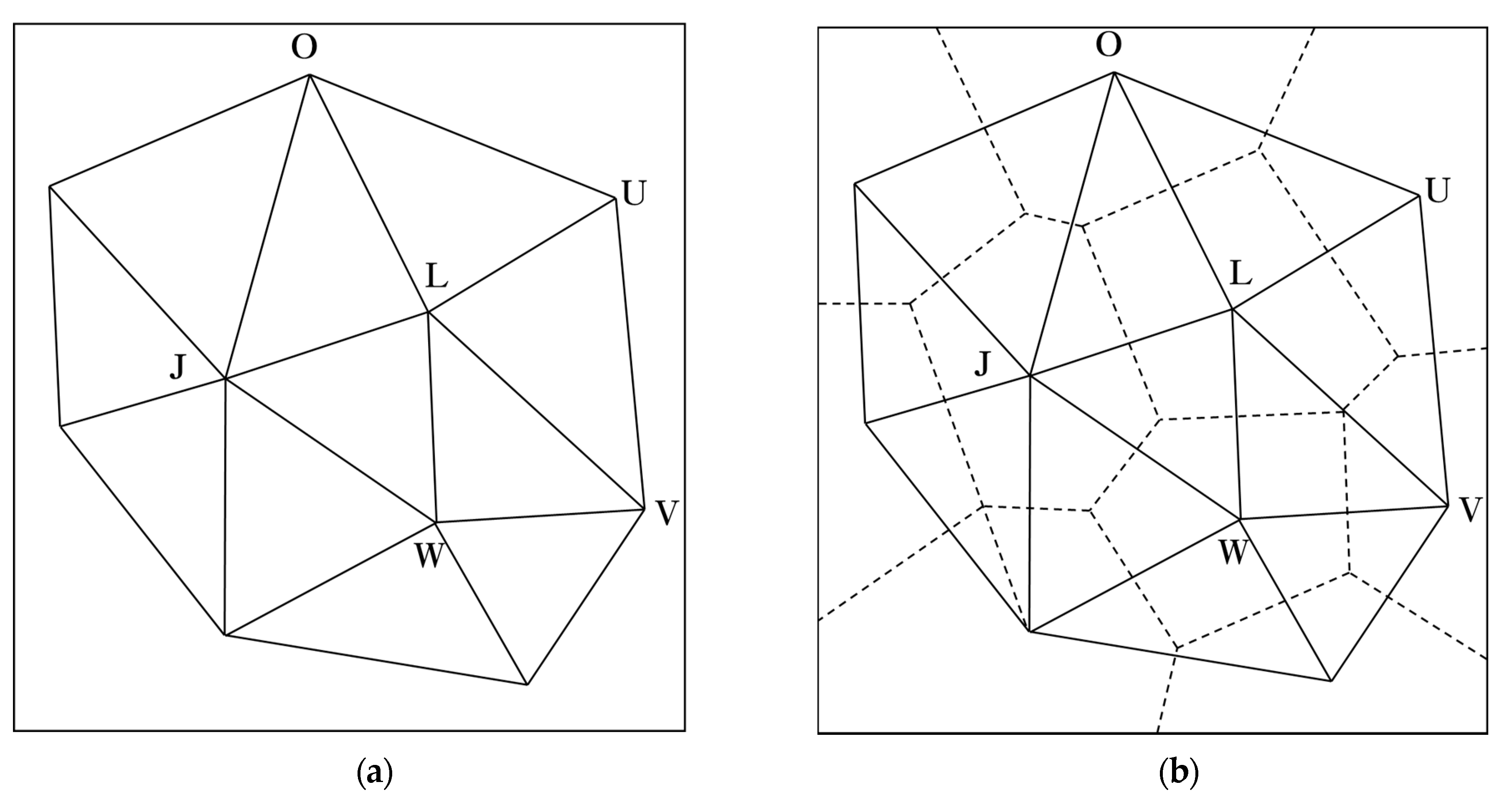
2.2. Thiessen Method
2.3. Cluster Analysis
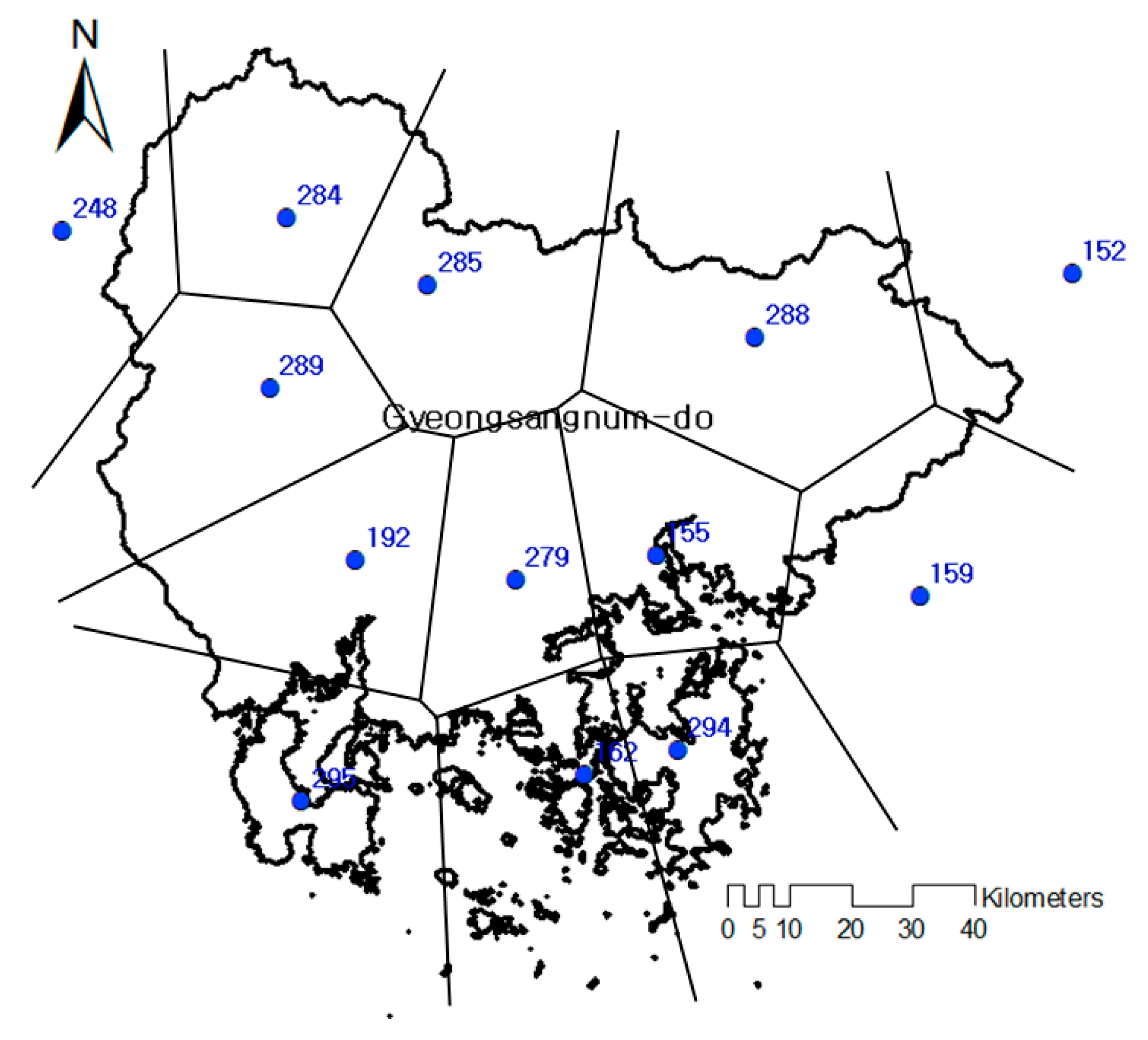
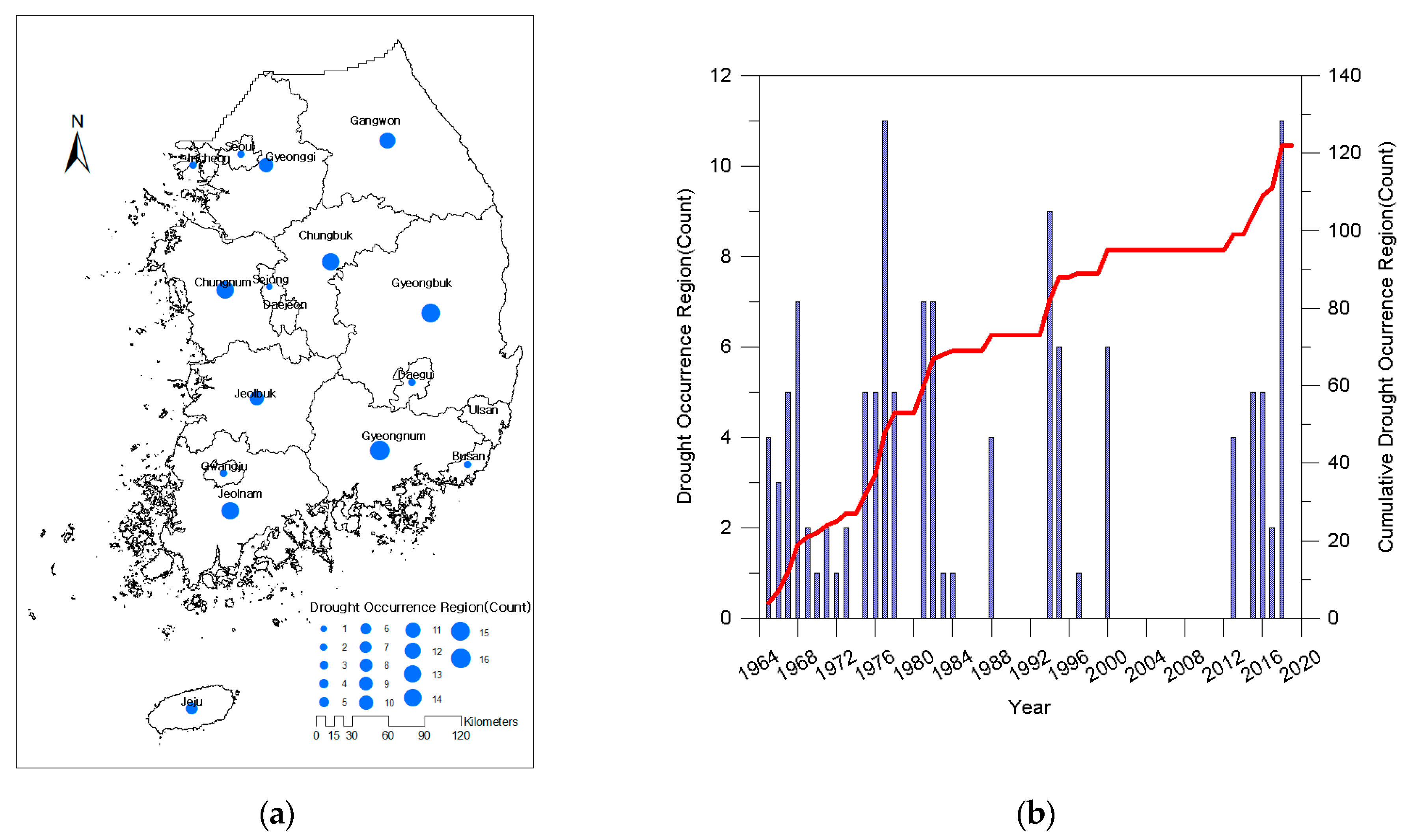
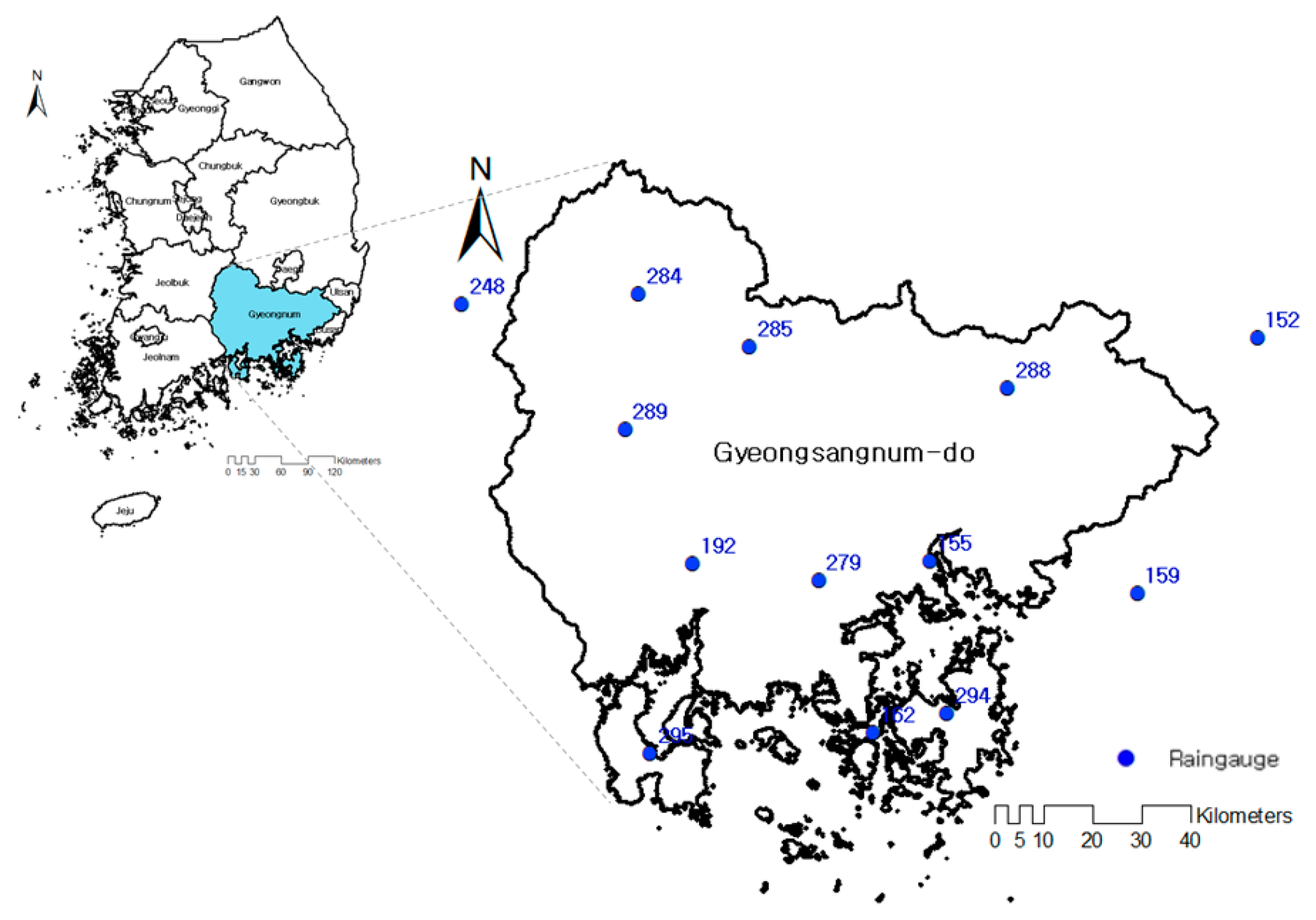
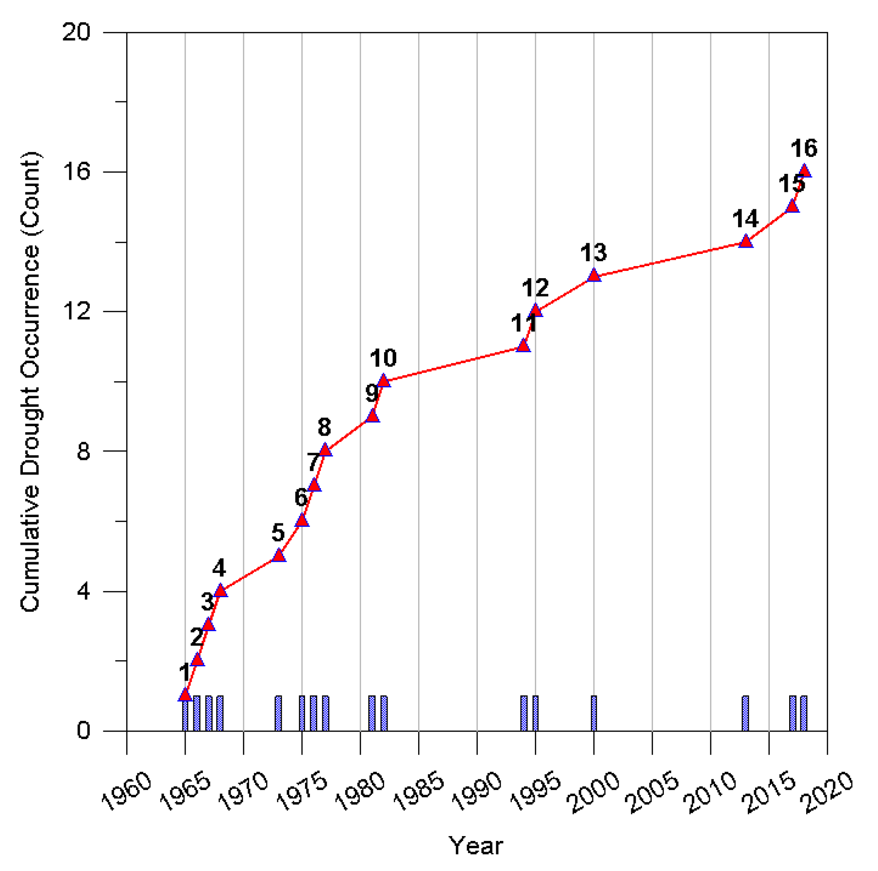
2.4. Drought Damage Status and Target Area Selection
3. Results
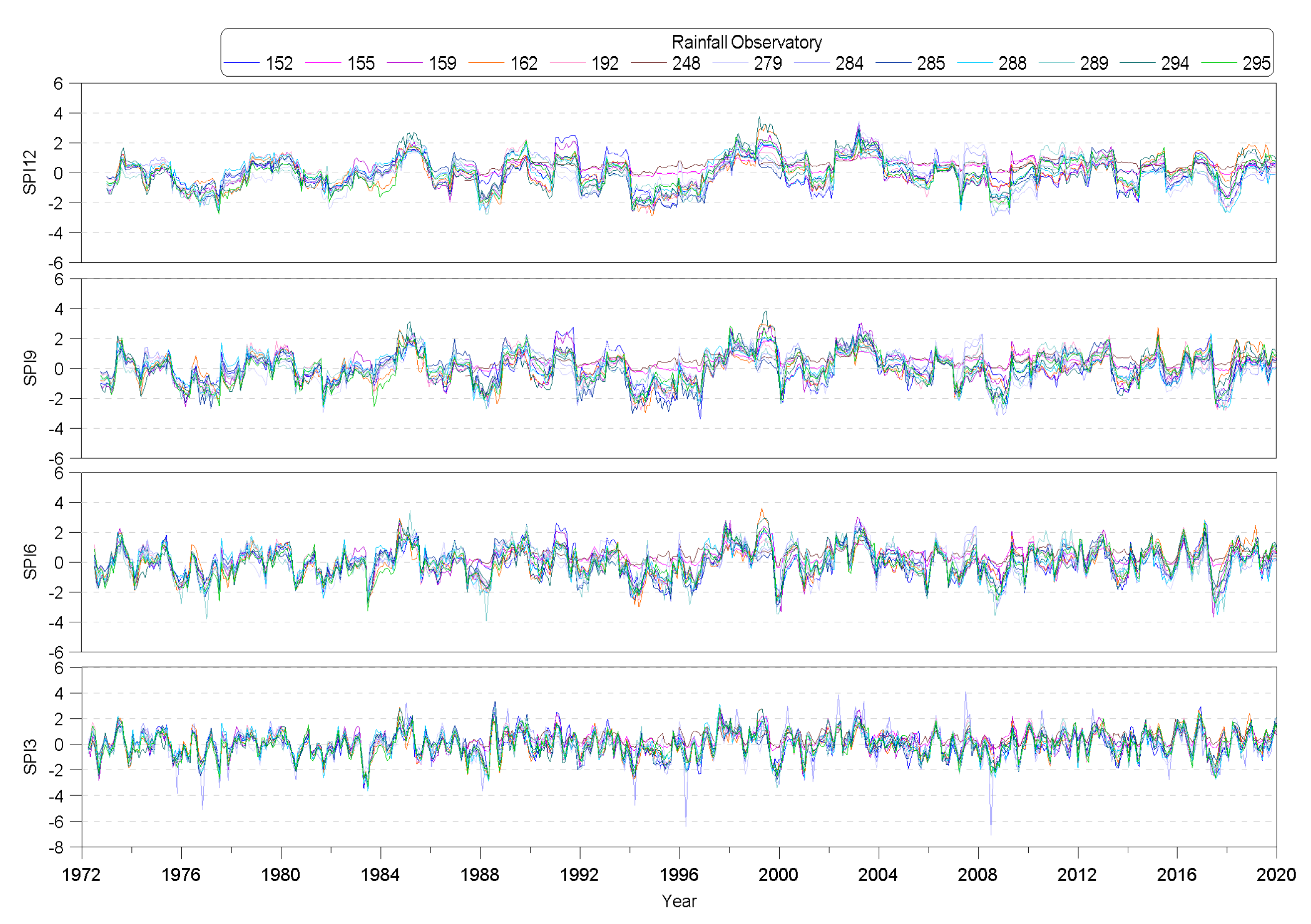
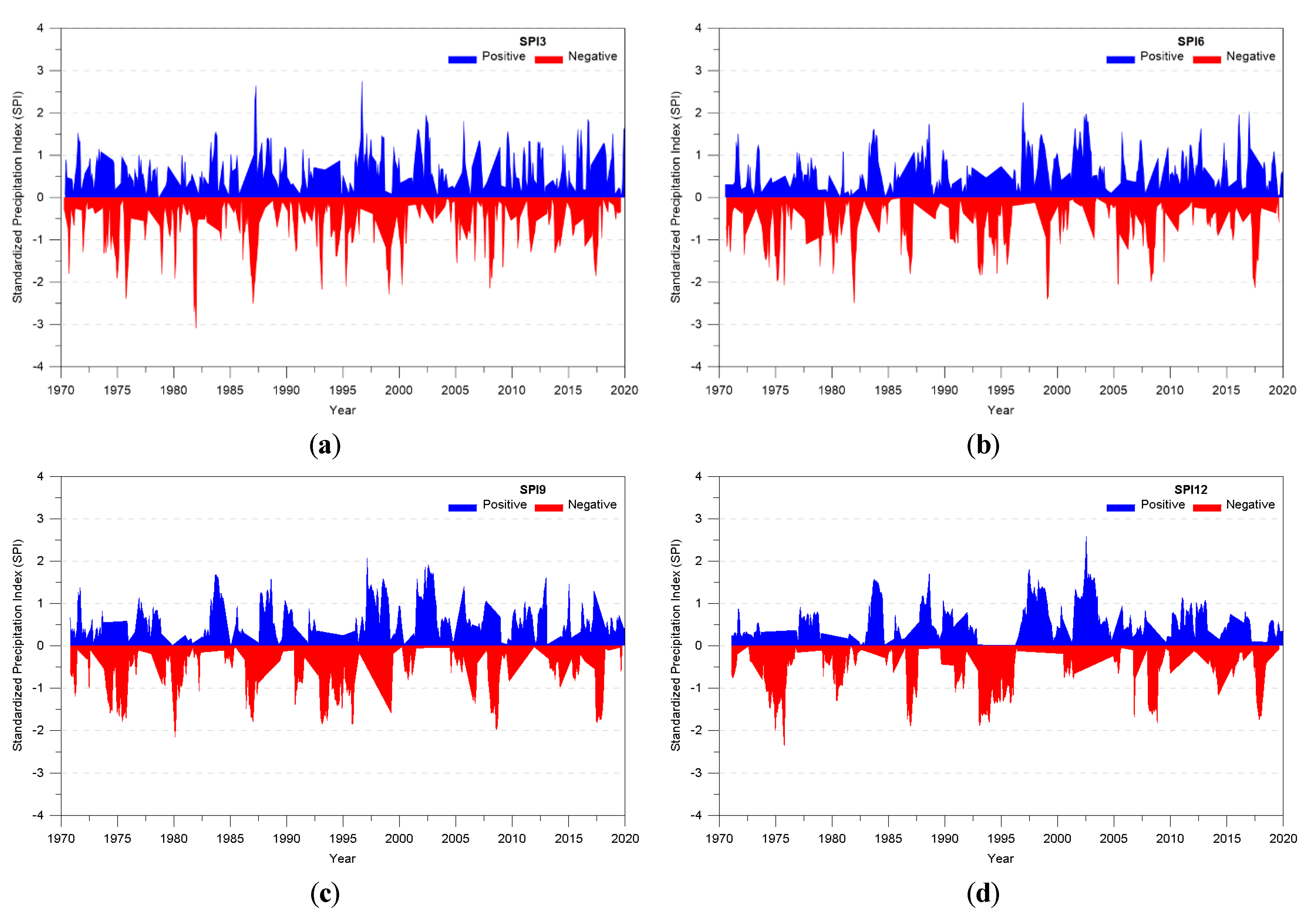
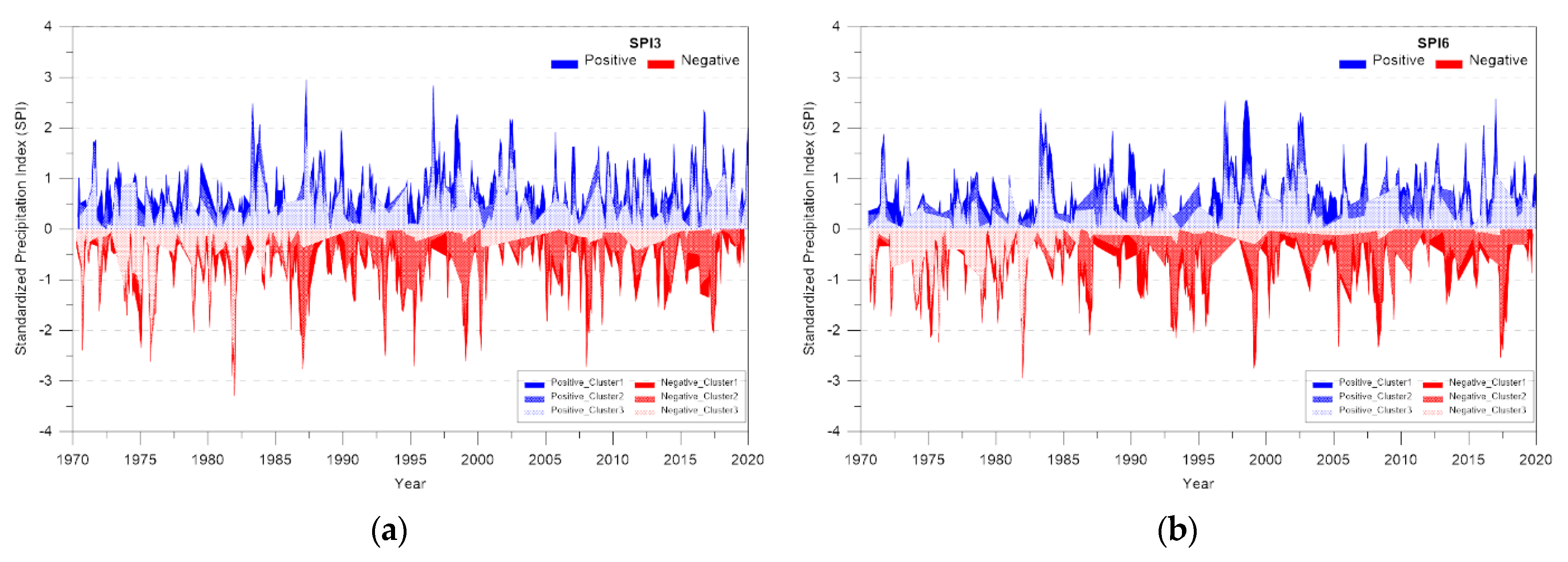
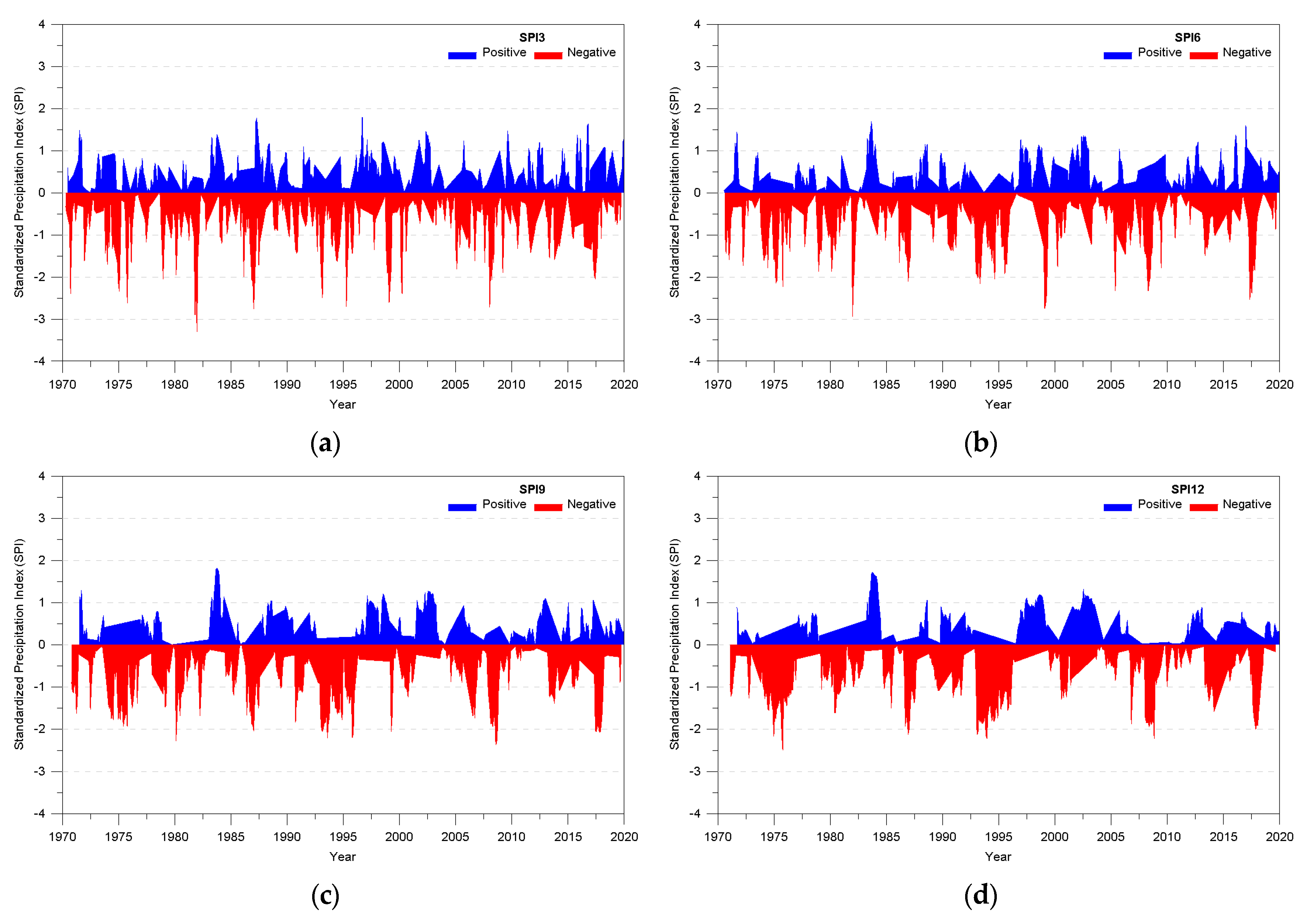
3.1. SPI Analysis
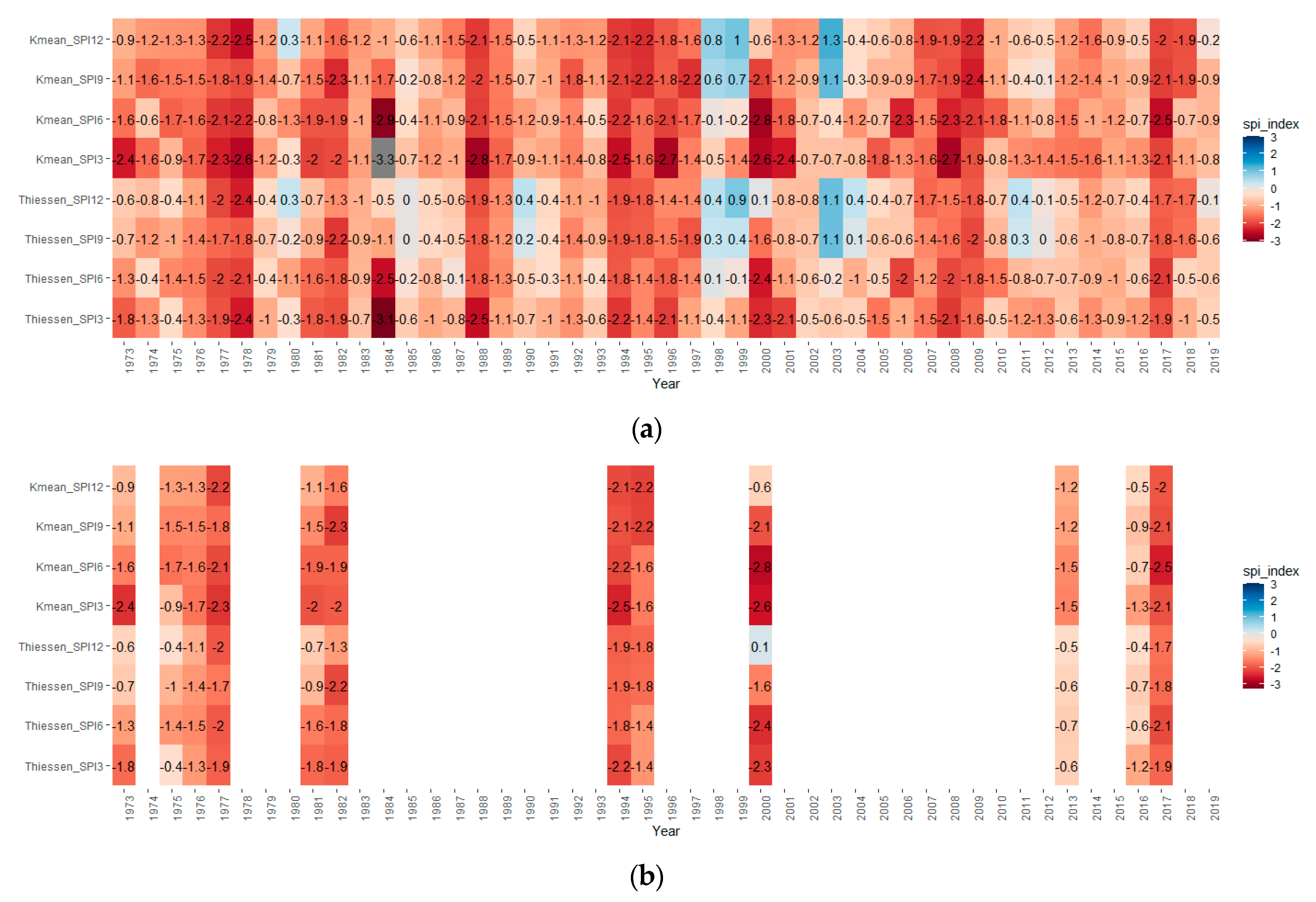
3.2. Drought Index Analysis Using the Thiessen Method
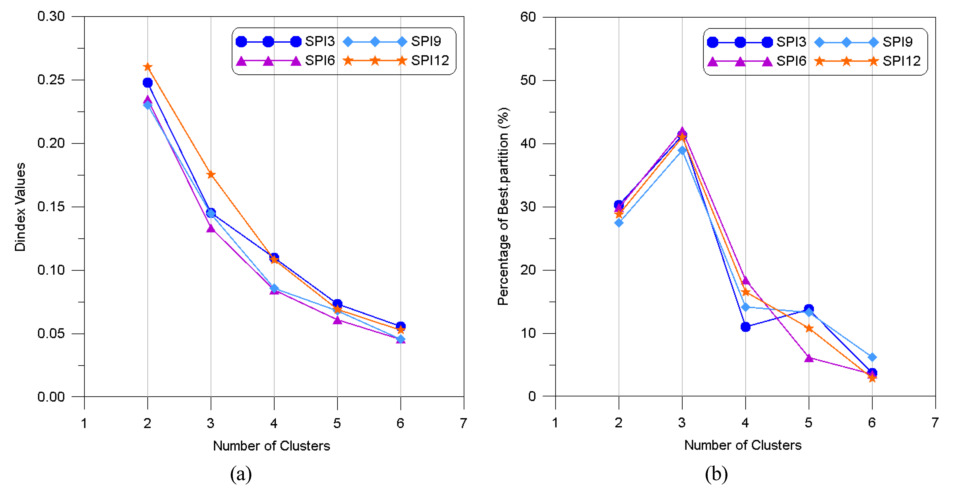
3.3. Analysis of the Drought Index Using Cluster Analysis
3.4. Examination of Drought Damage and the Appropriateness of the Drought Index
4. Discussion
5. Conclusions
Author Contributions
Funding
Informed Consent Statement
Data Availability Statement
Acknowledgments
Conflicts of Interest
References
- Rossi, G.; Benedini, M.; Tsakiris, G.; Giakoumakis, S. On regional drought estimation and analysis. Water Resour. Manag. 1992, 6, 249–277. [Google Scholar] [CrossRef]
- Obasi, G.O.P. Wmo’s role in the international decade for natural disaster reduction. Bull. Am. Meteorol. Soc. 1994, 75, 1655–1661. [Google Scholar] [CrossRef] [Green Version]
- Mpelasoka, F.; Hennessy, K.; Jones, R.; Bates, B. Comparison of suitable drought indices for climate change impacts assessment over australia towards resource management. Int. J. Climatol. 2008, 28, 1283–1292. [Google Scholar] [CrossRef]
- McKee, T.B.; Doesken, N.J.; Kleist, J. The relationship of drought frequency and duration to time scales. In Proceedings of the 8th Conference on Applied Climatology, Anaheim, CA, USA, 17–22 January 1993; American Meteorological Society: Boston, MA, USA, 1993; Volume 17, pp. 179–183. [Google Scholar]
- Vicente-Serrano, S.M.; Beguería, S.; López-Moreno, J.I. A multiscalar drought index sensitive to global warming: The standardized precipitation evapotranspiration index. J. Clim. 2010, 23, 1696–1718. [Google Scholar] [CrossRef] [Green Version]
- Tsakiris, G.; Vangelis, H. Establishing a drought index incorporating evapotranspiration. Eur. Water 2005, 9, 3–11. [Google Scholar]
- Palmer, W.C. Meteorological Drought; US Department of Commerce, Weather Bureau: Washington, DC, USA, 1965. [Google Scholar]
- Byun, H.-R.; Wilhite, D.A. Objective quantification of drought severity and duration. J. Clim. 1999, 12, 2747–2756. [Google Scholar] [CrossRef]
- Hayes, M.; Svoboda, M.; Wall, N.; Widhalm, M. The lincoln declaration on drought indices: Universal meteorological drought index recommended. Bull. Am. Meteorol. Soc. 2011, 92, 485–488. [Google Scholar] [CrossRef] [Green Version]
- Livada, I.; Assimakopoulos, V. Spatial and temporal analysis of drought in Greece using the standardized precipitation index (SPI). Theor. Appl. Climatol. 2007, 89, 143–153. [Google Scholar] [CrossRef]
- Smakhtin, V.; Hughes, D. Automated estimation and analyses of meteorological drought characteristics from monthly rainfall data. Environ. Model Softw. 2007, 22, 880–890. [Google Scholar] [CrossRef]
- Naresh Kumar, M.; Murthy, C.; Sesha Sai, M.; Roy, P. On the use of standardized precipitation index (SPI) for drought intensity assessment. Meteorol. Appl. 2009, 16, 381–389. [Google Scholar] [CrossRef] [Green Version]
- Kisi, O.; Gorgij, A.; Zounemat-Kermani, M.; Mahdavi-Meymand, A.; Kim, S. Drought forecasting using novel heuristic methods in a semi-arid environment. J. Hydrol. 2019, 578, 124053. [Google Scholar] [CrossRef]
- Agnew, C.T.; Chappell, A. Drought in the Sahel. GeoJournal 1999, 48, 299–311. [Google Scholar] [CrossRef]
- Cheo, A.E.; Voigt, H.J.; Mbua, R.L. Vulnerability of water resources in northern Cameroon in the context of climate change. Environ. Earth Sci. 2013, 70, 1211–1217. [Google Scholar] [CrossRef]
- Dhakar, R.; Sehgal, V.K.; Pradhan, S. Study on inter-seasonal and intra-seasonal relationships of meteorological and agricultural drought indices in the Rajasthan State of India. J. Arid. Environ. 2013, 97, 108–119. [Google Scholar] [CrossRef]
- Dutra, E.; Di Giuseppe, F.; Wetterhall, F.; Pappenberger, F. Seasonal forecasts of droughts in African basins using the Standardized Precipitation Index. Hydrol. Earth Syst. Sci. 2013, 17, 2359–2373. [Google Scholar] [CrossRef] [Green Version]
- Edossa, D.C.; Babel, M.S.; Gupta, A.D. Drought analysis in the Awash River basin, Ethiopia. Water Resour. Manag. 2010, 24, 1440–1460. [Google Scholar] [CrossRef]
- Feng, J.; Yan, D.H.; Li, C.Z. Evolutionary trends of drought under climate change in the Heihe River basin, Northwest China. J. Food Agric. Environ. 2013, 11, 1025–1031. [Google Scholar]
- Ford, T.; Labosier, C.F. Spatial patterns of drought persistence in the Southeastern United States. Int. J. Climatol. 2014, 34, 2229–2240. [Google Scholar] [CrossRef]
- Ganguli, P.; Reddy, M.J. Evaluation of trends and multivariate frequency analysis of droughts in three meteorological subdivisions of western India. Int. J. Climatol. 2014, 34, 911–928. [Google Scholar] [CrossRef]
- Gocic, M.; Trajkovic, S. Analysis of precipitation and drought data in Serbia over the period 1980–2010. J. Hydrol. 2013, 494, 32–42. [Google Scholar] [CrossRef]
- Hayes, M.J.; Svoboda, M.D.; Wihite, D.A.; Vanyarhko, O.V. Monitoring the 1996 drought using the standardized precipitation index. Bull. Am. Meteorol. Soc. 1999, 80, 429–438. [Google Scholar] [CrossRef] [Green Version]
- Karavitis, C.A.; Chortaria, C.; Alexandris, S.; Vasilakou, C.G.; Tsesmelis, D.E. Development of the standardised precipitation index for Greece. Urban Water J. 2012, 9, 401–417. [Google Scholar] [CrossRef]
- Khan, S.; Gabriel, H.F.; Rana, T. Standard precipitation index to track drought and assess impact of rainfall on watertables in irrigation areas. Irrig. Drain. Syst. 2008, 22, 159–177. [Google Scholar] [CrossRef]
- Liu, X.C.; Xu, Z.X.; Yu, R.H. Spatiotemporal variability of drought and the potential climatological driving factors in the Liao River basin. Hydrol. Process. 2012, 26, 1–14. [Google Scholar] [CrossRef]
- Lloyd-Hughes, B.; Saunders, M.A. A drought climatology for Europe. Int. J. Climatol. 2002, 22, 1571–1592. [Google Scholar] [CrossRef]
- Pai, D.S.; Sridhar, L.; Guhathakurta, P.; Hatwar, H.R. District-wide drought climatology of the southwest monsoon season over India based on standardized precipitation index (SPI). Nat. Hazards 2011, 59, 1797–1813. [Google Scholar] [CrossRef]
- Seiler, R.; Hayes, M.; Bressan, L. Using the standardized precipitation index for flood risk monitoring. Int. J. Climatol. 2002, 22, 1365–1376. [Google Scholar] [CrossRef]
- Spinoni, J.; Naumann, G.; Carrao, H.; Barbosa, P.; Vogt, J. World drought frequency, duration, and severity for 1951–2010. Int. J. Climatol. 2014, 34, 2792–2804. [Google Scholar] [CrossRef] [Green Version]
- Tabari, H.; Abghari, H.; Talaee, P.H. Temporal trends and spatial characteristics of drought and rainfall in arid and semiarid regions of Iran. Hydrol. Process. 2012, 26, 3351–3361. [Google Scholar] [CrossRef]
- Tsakiris, G.; Vangelis, H. Towards a drought watch system based on spatial SPI. Water Resour. Manag. 2004, 18, 1–12. [Google Scholar] [CrossRef]
- Vasiliades, L.; Loukas, A.; Liberis, N. A water balanced derived drought index for Pinios River Basin, Greece. Water Resour. Manag. 2010, 25, 1087–1101. [Google Scholar] [CrossRef]
- Vincente-Serrano, S.M.; Gonzalez-Hidalgo, J.C.; Luis, M.; Raventos, J. Drought pattern in the Mediterranean area: The Valencia region (eastern Spain). Clim. Res. 2004, 26, 5–15. [Google Scholar] [CrossRef] [Green Version]
- Xie, H.; Ringler, C.; Zhu, T.J.; Waqas, A. Droughts in Pakistan: A spatiotemporal variability analysis using the Standardized Precipitation Index. Water Int. 2013, 38, 620–631. [Google Scholar] [CrossRef]
- Zhang, Q.; Li, J.F.; Singh, V.P.; Bai, Y.G. SPI-based evaluation of drought events in Xinjiang, China. Nat. Hazards 2012, 64, 481–492. [Google Scholar] [CrossRef]
- Zin, W.Z.W.; Jemain, A.A.; Ibrahim, K. Analysis of drought condition and risk in Peninsular Malaysia using Standardised Precipitation Index. Theor. Appl. Climatol. 2013, 111, 559–568. [Google Scholar] [CrossRef]
- Zhang, Q.; Xu, C.Y.; Zhang, Z.X. Observed changes of drought/wetness episodes in the Pearl River basin, China, using the standardized precipitation index and aridity index. Theor. Appl. Climatol. 2009, 98, 89–99. [Google Scholar] [CrossRef]
- Du, J.; Fang, J.; Xu, W.; Shi, P.J. Analysis of dry/wet conditions using the standardized precipitation index and its potential usefulness for drought/flood monitoring in Hunan Province, China. Stoch. Environ. Res. Risk Assess. 2013, 27, 377–387. [Google Scholar] [CrossRef]
- Fischer, T.; Gemmer, M.; Su, B.; Scholten, T. Hydrological long-term dry and wet periods in the Xijiang River basin, South China. Hydrol. Earth Syst. Sci. 2013, 17, 135–148. [Google Scholar] [CrossRef] [Green Version]
- Huang, J.; Sun, S.L.; Xue, Y.; Li, J.J.; Zhang, J.C. Spatial and Temporal Variability of Precipitation and Dryness/Wetness during 1961–2008 in Sichuan province, West China. Water Resour. Manag. 2014, 28, 1655–1670. [Google Scholar] [CrossRef]
- Raziei, T.; Bordi, I.; Pereira, L.S.; Corte-Real, J.; Santos, J.A. Relationship between daily atmospheric circulation types and winter dry/wet spells in western Iran. Int. J. Climatol. 2012, 32, 1056–1068. [Google Scholar] [CrossRef] [Green Version]
- Tosic, I.; Unkasevic, M. Analysis of wet and dry periods in Serbia. Int. J. Climatol. 2014, 34, 1357–1368. [Google Scholar] [CrossRef]
- Li, B.; Su, H.B.; Chen, F.; Li, S.G.; Tian, J.; Qin, Y.C.; Zhang, R.H.; Chen, S.H.; Yang, Y.M.; Rong, Y. The changing pattern of droughts in the Lancang River Basin during 1960–2005. Theor. Appl. Climatol. 2013, 111, 401–415. [Google Scholar] [CrossRef]
- Zhao, G.J.; Mu, X.M.; Hormann, G.; Fohrer, N.; Xiong, M.; Su, B.D.; Li, X.C. Spatial patterns and temporal variability of dryness/wetness in the Yangtze River Basin, China. Quat. Int. 2012, 282, 5–13. [Google Scholar] [CrossRef]
- Bokal, S. Standardized Precipitation Index Tool for Drought Monitoring—Examples from Slovenia, Drought Management Centre for South-Eastern Europe; DMCSEE: Ljubljana, Slovenia, 2017. [Google Scholar]
- Santos, J.F.; Pulido-Calvo, I.; Portela, M.M. Spatial and temporal variability of drought in Portugal. Water Resour. Res. 2010, 46, W03503. [Google Scholar] [CrossRef] [Green Version]
- Moreira, E.E.; Martins, D.S.; Pereira, L.S. Assessing drought cycles in SPI time series using a Fourier analysis. NHESS 2015, 15, 571–585. [Google Scholar] [CrossRef] [Green Version]
- Mishra, A.K.; Singh, V.P. A review of drought concepts. J. Hydrol. 2010, 391, 202–216. [Google Scholar] [CrossRef]
- val Loon, A.F.; Laaha, G. Hydrological drought severity explained by climate and catchment characteristics. J. Hydrol. 2015, 526, 3–14. [Google Scholar] [CrossRef] [Green Version]
- Barker, L.; Hannaford, J.; Chiverton, A.; Svensson, C. From meteorological to hydrological drought using standardized indicators. Hydrol. Earth Syst. Sci. 2016, 20, 2483–2505. [Google Scholar] [CrossRef] [Green Version]
- Mavromatis, T. Drought index evaluation for assessing future wheat production in Greece. Int. J. Climatol. 2007, 27, 911–924. [Google Scholar] [CrossRef]
- Kempes, C.; Myers, O.; Breshears, D.; Ebersole, J. Comparing response of Pinus edulis tree-ring growth to five alternate moisture indices using historic meteorological data. J. Arid Environ. 2008, 72, 350–357. [Google Scholar] [CrossRef]
- Vicente-Serrano, S.; Beguería, S.; López-Moreno, J.; Angulo, M.; El Kenawy, A. A new global 0.5 gridded dataset (1901–2006) of a multiscalar drought index: Comparison with current drought index datasets based on the Palmer Drought Severity Index. J. Hydrometeorol. 2010, 11, 1033–1043. [Google Scholar] [CrossRef] [Green Version]
- Taylor, C.; de Jeu, R.; Guichard, F.; Harris, P.; Dorigo, W. Afternoon rain more likely over drier soils. Nature 2012, 489, 423–426. [Google Scholar] [CrossRef] [Green Version]
- Teuling, A.; Van Loon, A.; Seneviratne, S.; Lehner, I.; Aubinet, M.; Heinesch, B.; Spank, U. Evapotranspiration amplifies European summer drought. Geophys. Res. Lett. 2013, 40, 2071–2075. [Google Scholar] [CrossRef]
- Zhang, B.; He, C. A modified water demand estimation method for drought identification over arid and semiarid regions. Agric. For. Meteorol. 2016, 230, 58–66. [Google Scholar] [CrossRef]
- Asrari, E.; Masoudi, M. A new methodology for drought vulnerability assessment using SPI (standardized precipitation index). Int. J. Sci. Knowl. 2014, 2, 425–432. [Google Scholar] [CrossRef]
- Masoudi, M.; Hakimi, S. A new model for vulnerability assessment of drought in Iran using percent of normal precipitation index (PNPI). Iran. J. Sci. Technol. Sci. 2014, 38, 435–440. [Google Scholar]
- Zarei, A.; Masoudi, M.; Mahmodi, A.R. Analyzing spatial pattern of drought changes in Iran, using standardized precipitation index (SPI). Ecol. Environ. Conserv. 2014, 20, 427–432. [Google Scholar]
- Won, J.; Choi, J.; Lee, O.; Kim, S. Copula-based joint drought index using SPI and EDDI and its application to climate change. Sci. Total Environ. 2020, 744, 140701. [Google Scholar] [CrossRef]
- Rhee, J.; Carbone, G.J.; Hussey, J. Drought index mapping at different spatial units. J. Hydrometeorol. 2008, 9, 1523–1534. [Google Scholar] [CrossRef]
- Thomas, B.F.; Famiglietti, J.S.; Landerer, F.W.; Wiese, D.N.; Molotch, N.P.; Argus, D.F. GRACE groundwater drought index: Evaluation of California Central Valley groundwater drought. Remote. Sens. Environ. 2017, 198, 384–392. [Google Scholar] [CrossRef]
- Zhang, H.; Song, J.; Wang, G.; Wu, X.; Li, J. Spatiotemporal characteristic and forecast of drought in northern Xinjiang, China. Ecol. Indic. 2021, 127, 107712. [Google Scholar] [CrossRef]
- Zhou, H.; Liu, Y. SPI based meteorological drought assessment over a humid basin: Effects of processing schemes. Water 2016, 8, 373. [Google Scholar] [CrossRef] [Green Version]
- Zhai, J.; Su, B.; Krysanova, V.; Vetter, T.; Gao, C.; Jiang, T. Spatial variation and trends in PDSI and SPI indices and their relation to streamflow in 10 large regions of China. J. Clim. 2010, 23, 649–663. [Google Scholar] [CrossRef]
- Gao, L.; Zhang, Y. Spatio-temporal variation of hydrological drought under climate change during the period 1960–2013 in the Hexi Corridor, China. J. Arid Land 2016, 8, 157–171. [Google Scholar] [CrossRef] [Green Version]
- Dash, B.K.; Rafiuddin, M.; Khanam, F.; Islam, M.N. Characteristics of meteorological drought in Bangladesh. Nat. Hazards 2012, 64, 1461–1474. [Google Scholar] [CrossRef]
- Mishra, A.K.; Singh, V.P.; Desai, V.R. Drought characterization: A probabilistic approach. Stoch. Environ. Res. Risk Assess. 2007, 23, S11–S19. [Google Scholar] [CrossRef]
- Vicente-Serrano, S.M. Differences in spatial patterns of drought on different time scales: An analysis of the Iberian Peninsula. Water Resour. Manag. 2006, 20, 37–60. [Google Scholar] [CrossRef]
- Shamshirband, S.; Gocić, M.; Petković, D.; Javidnia, H.; Ab Hamid, S.H.; Mansor, Z.; Qasem, S.N. Clustering project management for drought regions determination: A case study in Serbia. Agric. For. Meteorol. 2015, 200, 57–65. [Google Scholar] [CrossRef]
- McKee, T.B. Drought Monitoring with Multiple Time Scales. In Proceedings of the 9th Conference on Applied Climatology, Boston, MA, USA, 15–20 January 1995. [Google Scholar]
- Rebay, S. Efficient Unstructured mesh generation by mean of Delaunay triangulation and Bowyer-Watson algorithm. J. Comput. Phys. 1993, 106, 125–138. [Google Scholar] [CrossRef]
- Pedrini, H. An Adaptive Method for Terrain Surface Approximation Based on Triangular Meshes. Ph.D. Thesis, Rensselaer Institute Troy, New York, NY, USA, 2000. [Google Scholar]
- MacQueen, J. Some Methods for Classification and Analysis of Multivariate Observation, in 5th Berkeley Symposium on Mathematical Statistics and Probability; Statistical Laboratory University: California, CA, USA, 1967; pp. 281–297. [Google Scholar]
- Lloyd, S. Least squares quantization in PCM. IEEE Trans. Inf. Theory 1982, 28, 129–137. [Google Scholar] [CrossRef]
- Trenberth, K.; Overpeck, J.; Solomon, S. Exploring drought and its implications for the future. EOS Trans. Am. Geophys. Union 2007, 85, 27. [Google Scholar] [CrossRef]


| SPI Values | Drought Category | Occurrence Probability (%) |
|---|---|---|
| 2.00 ≤ SPI | Extremely wet | 2.3 |
| 1.50–1.99 | Very wet | 4.4 |
| 1.00–1.49 | Moderately wet | 9.2 |
| −0.99–0.99 | Near normal | 68.2 |
| −1.49 to −1.00 | Moderately dry | 9.2 |
| −1.99 to −1.50 | Severe dry | 4.4 |
| SPI ≤ −2.00 | Extremely dry | 2.3 |
| Step | Contents |
|---|---|
| Step 1 | Initial k clusters are selected from n data. |
| Step 2 | Data are composed of the nearest k clusters. |
| Step 3 | k clusters are created arbitrarily, and the initial values are estimated for the average of each cluster, i.e., |
| Step 4 | The average of n data in k clusters is calculated. |
| Step 5 | Steps 3 and 4 are repeated until there is no significant change in the average. |
| Station Index | Station Name | Observation Date | Station Index | Station Name | Observation Date |
|---|---|---|---|---|---|
| 152 | Ulsan | 1965.01 | 284 | Geochang | 1972.01 |
| 155 | Changwon | 1985.07 | 285 | Hapcheon | 1973.01 |
| 159 | Busan | 1965.01 | 288 | Miryang | 1973.01 |
| 162 | Tongyeong | 1968.01 | 289 | Sancheong | 1972.03 |
| 192 | Jinju | 1969.03 | 294 | Geoje | 1972.01 |
| 248 | Jangju | 1988.01 | 295 | Namhae | 1972.01 |
| 279 | Gumi | 1973.01 | Count | 13 | |
| Station Index | Station Name | Thiessen Weight | Station Index | Station Name | Thiessen Weight | ||
|---|---|---|---|---|---|---|---|
| 1973−1987 | 1988−2019 | 1973−1987 | 1988−2019 | ||||
| 152 | Ulsan | 0.019 | 0.016 | 284 | Geochang | - | 0.107 |
| 155 | Changwon | - | 0.088 | 285 | Hapcheon | 0.147 | 0.118 |
| 159 | Busan | 0.034 | 0.028 | 288 | Miryang | 0.193 | 0.155 |
| 162 | Tongyeong | 0.044 | 0.036 | 289 | Sancheong | 0.150 | 0.120 |
| 192 | Jinju | 0.155 | 0.126 | 294 | Geoje | 0.046 | 0.037 |
| 248 | Jangju | 0.027 | 0.021 | 295 | Namhae | 0.066 | 0.053 |
| 279 | Gumi | 0.119 | 0.095 | Sum | 1.000 | 1.000 | |
| Drought Index | MAD | MSE | RMSE | Drought Index | MAD | MSE | RMSE | ||
|---|---|---|---|---|---|---|---|---|---|
| Thiessen | SPI3 | 0.523 | 0.506 | 0.711 | K-mean | SPI3 | 0.414 | 0.381 | 0.617 |
| SPI6 | 0.544 | 0.484 | 0.696 | SPI6 | 0.428 | 0.394 | 0.628 | ||
| SPI9 | 0.674 | 0.569 | 0.754 | SPI9 | 0.426 | 0.355 | 0.596 | ||
| SPI12 | 0.964 | 0.848 | 0.921 | SPI12 | 0.670 | 0.582 | 0.763 | ||
Publisher’s Note: MDPI stays neutral with regard to jurisdictional claims in published maps and institutional affiliations. |
© 2021 by the authors. Licensee MDPI, Basel, Switzerland. This article is an open access article distributed under the terms and conditions of the Creative Commons Attribution (CC BY) license (https://creativecommons.org/licenses/by/4.0/).
Share and Cite
Song, Y.; Park, M. A Study on the Appropriateness of the Drought Index Estimation Method Using Damage Data from Gyeongsangnamdo, South Korea. Atmosphere 2021, 12, 998. https://doi.org/10.3390/atmos12080998
Song Y, Park M. A Study on the Appropriateness of the Drought Index Estimation Method Using Damage Data from Gyeongsangnamdo, South Korea. Atmosphere. 2021; 12(8):998. https://doi.org/10.3390/atmos12080998
Chicago/Turabian StyleSong, Youngseok, and Moojong Park. 2021. "A Study on the Appropriateness of the Drought Index Estimation Method Using Damage Data from Gyeongsangnamdo, South Korea" Atmosphere 12, no. 8: 998. https://doi.org/10.3390/atmos12080998
APA StyleSong, Y., & Park, M. (2021). A Study on the Appropriateness of the Drought Index Estimation Method Using Damage Data from Gyeongsangnamdo, South Korea. Atmosphere, 12(8), 998. https://doi.org/10.3390/atmos12080998