Article

A Modeling Study on the Downslope Wind of “Katevatos” in Greece and Implications for the Battle of Arachova in 1826

by
Stavros Solomos
1,*,
Panagiotis T. Nastos
2,
Dimitrios Emmanouloudis
3,4,
Antonia Koutsouraki
5 and
Christos Zerefos
1,6,7,8
1
Research Centre for Atmospheric Physics and Climatology, Academy of Athens, 10679 Athens, Greece
2
Laboratory of Climatology and Atmospheric Environment, Department of Geology and Geoenvironment, National and Kapodistrian University of Athens, 15772 Athens, Greece
3
UNESCO Chair Con-E-Ect on Conservation & Ecotourism of Riparian & Deltaic Ecosystems, 66100 Drama, Greece
4
Department of Forestry and Natural Environment, International Hellenic University, 66100 Drama, Greece
5
Laboratory of Analysis and Management of Natural Disasters and Technological Risks, International Hellenic University, 66100 Drama, Greece
6
Biomedical Research Foundation, Academy of Athens, 11527 Athens, Greece
7
Navarino Environmental Observatory (N.E.O.), Costa Navarino, Navarino Dunes Messinia, 24001 Messinia, Greece
8
Mariolopoulos-Kanaginis Foundation for the Environmental Sciences, 10675 Athens, Greece
*
Author to whom correspondence should be addressed.
Atmosphere 2021, 12(8), 993; https://doi.org/10.3390/atmos12080993
Submission received: 30 June 2021 / Revised: 26 July 2021 / Accepted: 29 July 2021 / Published: 31 July 2021

Abstract

:
Downslope winds and lee gravity waves are common features of mountainous environments. A similar weather type at Mt. Parnassos in Arachova, Greece is known as “Katevatos” and has devastating results for the population and visitors at the local touristic resorts. In this study, we analyze three incidents of this atmospheric pattern at local scale resolution (1 × 1 km) with WRF model. This is the first study of this local weather hazard, and the following key factors are identified. (I) The main synoptic forcing is the propagation of an upper-level trough from central Europe towards the Balkans. (II) The associated generation of a surface low-pressure system over the Aegean Sea results in a northeast flow in the lower troposphere that is perpendicular to the main topographic ridge of Mt. Parnassos. (III) Generation of gravity waves and downward reflection of wave energy at the critical level between the upper level flow and the undercutting northeast current result in the formation of “Katevatos” downslope wind at the lee side of the mountain. This hurricane-scale wind is accompanied with horizontal transport of frozen rain and snow from the mountain tops towards the village of Arachova. This wind pattern appeared also during the battle of Arachova in November 1826 between the Greek and Ottoman forces resulting in enormous casualties due to the adverse weather conditions.

1. Introduction

The year 2021 marks the anniversary for the 200 years since the Greek revolution of 1821 against the Ottoman Empire that gave birth to the modern-era Greek state. One of the most important conflicts during this revolution took place in November 1826 at the mountainous village of Arachova that is located at 1000 m elevation at the south slope of Mt. Parnassos. According to the historic sources, a severe weather type that was prevailing during these days included very low temperatures, gale-scale winds, and adverse snowstorm [1,2,3,4,5]. The Greek barracks during the battle were at the lower elevations, allowing the troops to take cover and protection inside the village houses, while the Ottoman forces remained at higher elevations at the mountain slopes and thus were exposed to the extreme weather. This condition resulted in an almost complete elimination of the Ottoman forces due to the cold, the wind, and the severe snowstorm. This specific pattern is well known to the locals as “Katevatos”, which obviously reflects the katabatic nature of the wind and the associated phenomena. However, we need to distinguish here that the term “katabatic” is commonly reserved in meteorology for weak to moderate flows that occur from the cooling of the air masses adjacent to a mountain slope, while “katevatos” is actually a hurricane-force downslope windstorm of great local importance with wind speeds reaching up to 100 km h−1.
In general, the complex topographic features of Greece including a 15,000 km long coastline, over 6000 islands and a mountainous inland with steep orography, canyons, valleys, etc., result in the generation of numerous local weather patterns. Nowadays, these unique sceneries are the attraction of millions of visitors from around the world. However, the formation of local scale weather types played an important role and affected the fate of several battles and wars throughout the long Greek history. An early example is already evident for the battle of Salamis in 480 B.C., when the Greek admirals took advantage of a local sea-breeze to defeat the Persian fleet in the straits of Salamis [6].
Several local katabatic winds are known worldwide (e.g., “Bora” in the Adriatic Sea [7], “Mistral” in south France (Rhone valley) [8], etc.) associated with the formation of mountain gravity waves. Foehn-type winds are also typical in mountainous regions (e.g., “Chinook” in the US Rocky Mountains [9], “Livas” in Crete [10], etc.). Due to their local nature, such flows are not commonly included in mesoscale forecasts and analysis fields [11]. For example, [12] describe how the formation of a Foehn flow over the leeward slopes of Crete can only be described at a modeling grid-space of 1 × 1 km or finer. As a result, the “Katevatos” wind that is discussed here has not yet been extensively analyzed, despite its great importance for civil protection at the very popular touristic destination of Arachova and its’ historic role. The specific area is one of the most important touristic destinations in Greece, attracting thousands of visitors per year due to winter sports activities but also due to the very important archaeological site of Delfi that is located 12 km west of Arachova. For this reason, apart from the profound scientific importance, a deeper understanding of this phenomenon is also needed in terms of civil security and protection against extreme weather events. In this study, we investigate the various physical processes that take place along several atmospheric scales (from synoptic to mesoscale and local) leading to the formation of this unique weather type. A conceptual approach of katabatic winds formation as well as the methodology used in this study are described in Section 2, followed by the analysis of our results in Section 3. Section 4 includes the conclusions as well as a discussion on the historical implications of “Katevatos”.

2. Theoretical Concept and Modeling Methodology

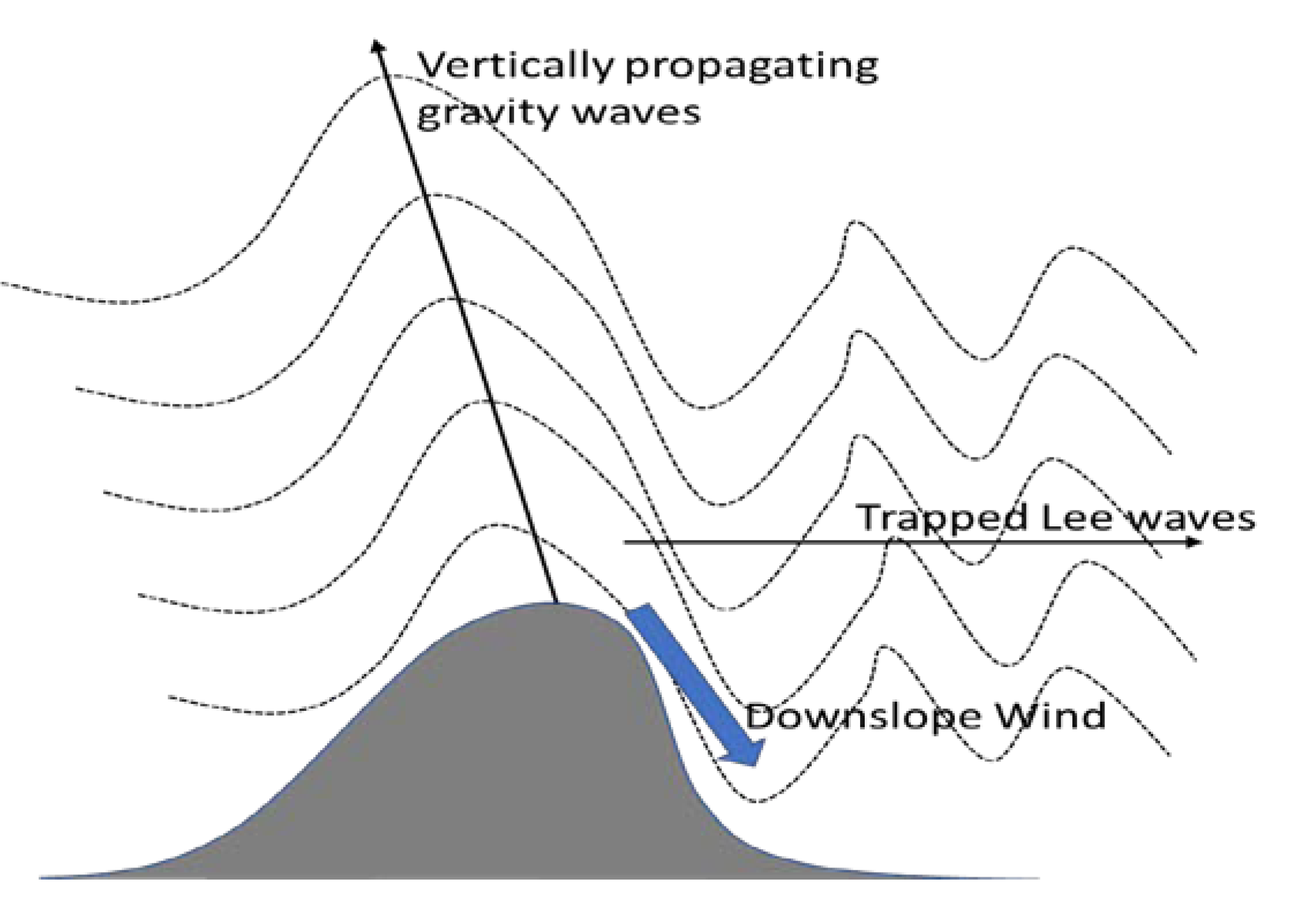
2.1. Theoretical Background

Formation of lee gravity waves is a common feature in atmospheric fluid dynamics. Lee waves form due to the vertical oscillation of the air mass, after the flow has been vertically perturbed to overcome a mountain ridge. The existence of such waves is often evident by the formation of lenticular clouds at the lee side of the mountain and by the generation of severe downslope winds (Figure 1). Considering Newton’s second law, the balance at the vertical direction takes the form of Equation (1), where z’ is the mean elevation of the air mass parcel, z is the vertical elevation, g is the gravitational constant and ρ is the density of the air mass. Assuming a vertically stabilized density field with denser fluid laying below the lighter ones and a constant rate of density change in the vertical ( ρ z < 0 ,   constant ) , Equation (1) obtains a solution in the wave form of Equation (2). This solution shows that the air mass parcel is oscillating in the vertical while traveling horizontally. Parameters A and B in Equation (2) are constants, and N is the classical Brunt-Vaisala frequency (Equation (3)) where θ is the potential temperature (e.g., [13]). In a stable air mass where N2 > 0 a vertically perturbed air parcel will have the tendency to come back to its equilibrium level, and the frequency of the oscillation is given by N. In an unstable air mass, N2 < 0 and the vertically perturbed air parcel will move away from the equilibrium level (i.e., free convection). Favorable tuning between atmospheric and topographic properties can lead to the formation of downslope windstorms analogous to a hydraulic jump when the flow over a mountain transitions from subcritical to supercritical, or when vertically-propagating mountain waves undergo partial reflection at wave-induced critical layers (wave breaking) or atmospheric critical layers (e.g., wind shear regimes) [14,15,16,17,18].
2 z t 2 = g ρ 0 ρ z z
z = A cos Ν t + B sin Ν t  
N = g θ θ z

2.2. Model Configuration

The modeling study is performed with WRF-ARW v4.1.3 model [19,20] set up in a 3-grid structure (12 × 12 km, 3 × 3 km, 1 × 1 km grid space) and 41 vertical sigma levels up to 50 mb. Initial and boundary fields are from the National Centers for Environmental Prediction (NCEP) final analysis dataset (FNL) at 1° × 1° resolution. The daily updated Sea Surface Temperature (SST) is from the NCEP 1° × 1° analysis. A 6 h spin-up time is assumed in all runs. The model microphysics are computed with the Morrison 2-moment scheme [21], shortwave and longwave radiation is computed with RRTMG scheme [22], the revised MM5 scheme and the NOAH Unified model are used for surface layer and soil physics, respectively [23,24], the YSU scheme is used for boundary layer physics [25] and the Grell 3D ensemble scheme [26,27] is used for cumulus parameterization.
Three separate runs are performed for the incidents of 13 February 2019, 6 January 2020 and 15 February 2021. The above days are selected due to their unusually high speeds and due to their characterization by the local community of Arachova as typical “Katevatos” events. For all three days, the recorded wind speed at the station of the National Observatory of Athens in Arachova [28] is the maximum monthly record. The station is located at elevation of 1069 m at 38°30′N, 22°36′E and the maximum recorded wind gusts during these events are 101.4 km h−1 at 21:20 UTC, 13 February 2019; 91.7 km h−1 at 01:10 UTC, 6 January 2020; and 77.2 km h−1 at 10:20 UTC, 15 February 2021. All the above extreme speeds are from N and NNE directions.

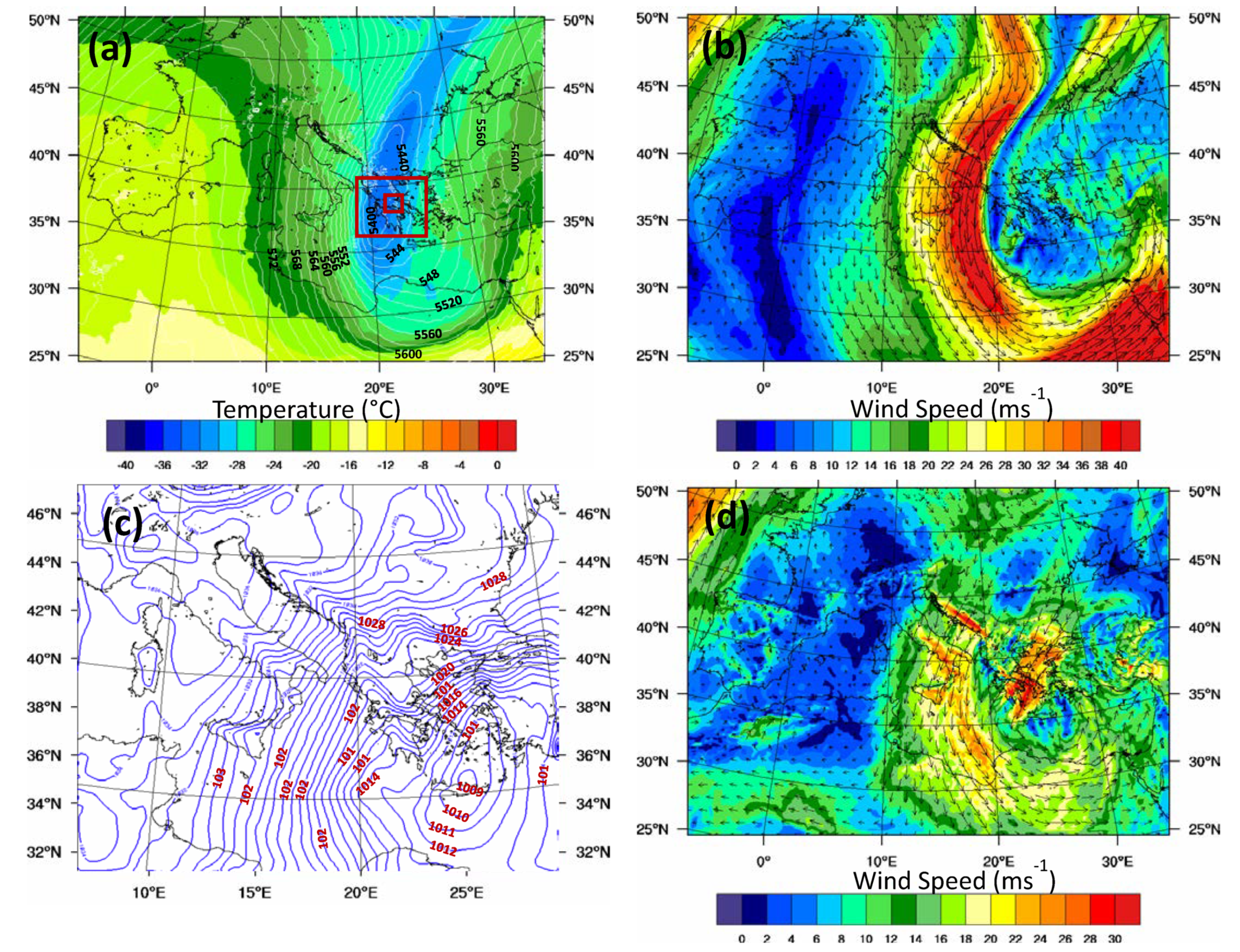
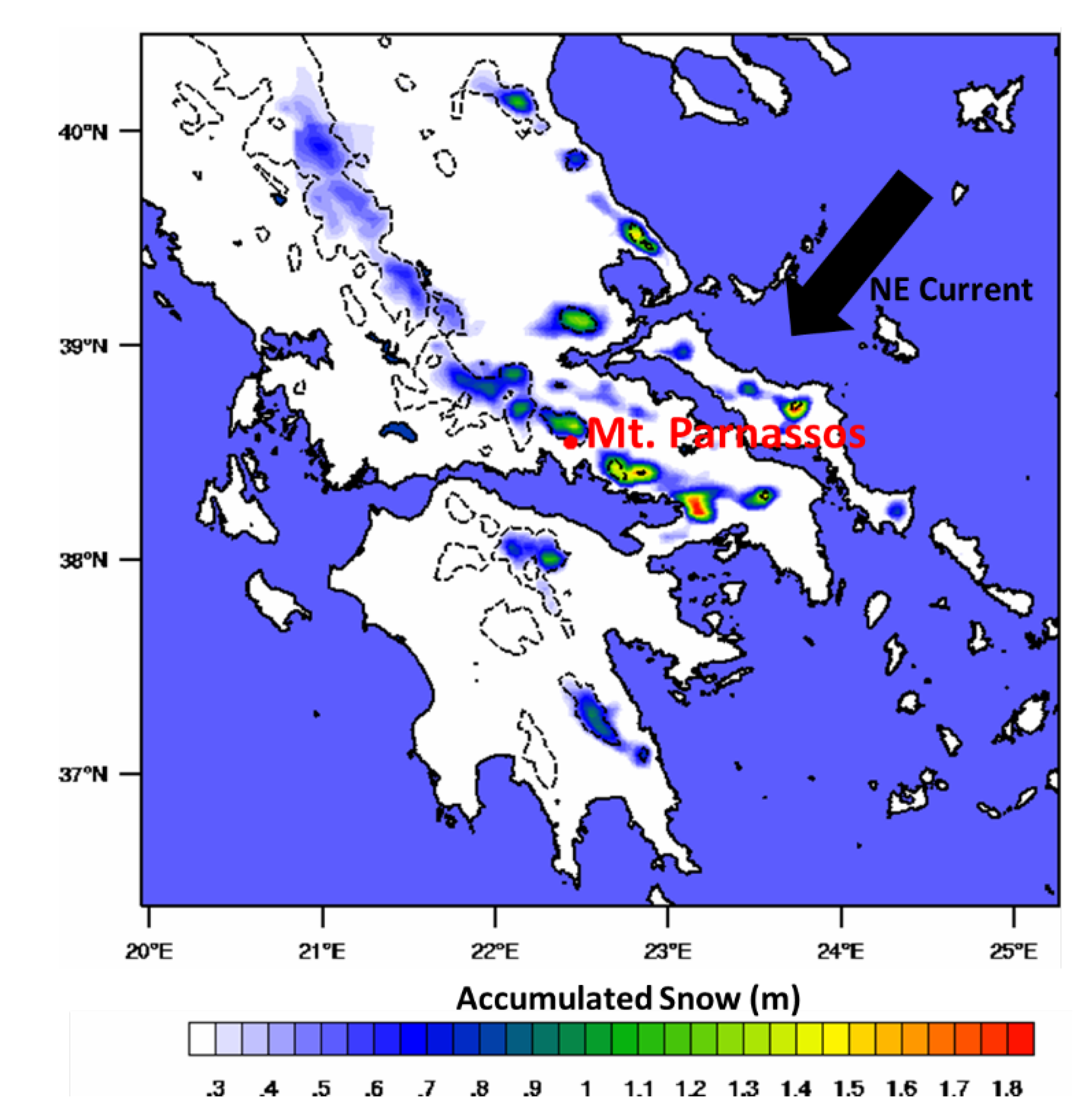
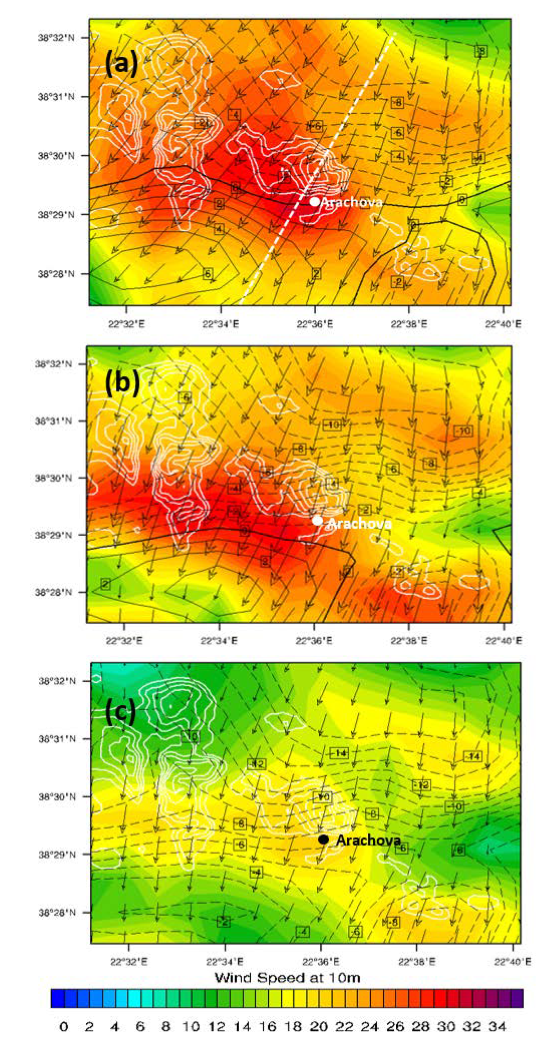
3. Modeling Results and Analysis of the Atmospheric Processes Forming “Katevatos”

The analysis is performed separately for the three cases of “Katevatos” in Arachova to identify the main atmospheric features that drive the phenomenon. All three events present similar findings in terms of the general atmospheric structure. For this reason, in the following paragraphs we present plots only from the February 2019 case, except when certain features are found to vary significantly between the runs. In such a case, separate plots are shown for each run to discuss similarities and differences.
At synoptic scale, the main atmospheric disturbance is found to be an eastward propagating trough that is evident by the geopotential height and temperature field at 500 mb in Figure 2a, on 13 February 2019, 18:00. The trough is deepening over Greece with geopotential heights reaching 5400 m and temperatures falling below −36 °C. The wind flow at 500 mb is dominated by the trough circulation, and as seen by the wind field on 14 February 2019, 00:00 UTC in Figure 2b, the wind direction over central Greece at this tropospheric level is SSE. Cyclogenesis is evident at the lower tropospheric levels on 14 February 2019, 00:00 UTC, as seen by the sea level pressure contours in Figure 2c. The center of the surface depression is found over the southern parts of Aegean Sea, accompanied by the “packing” of isobars along the SW–NE axis over the Aegean. The combination of this low-pressure system with the higher sea- level pressure over central Europe results in the generation of a strong northeast wind flow channeling through the Aegean with maximum speeds on 14 February 2019, 00:00 UTC exceeding 30 m s−1 at 850 mb (Figure 2d). The acceleration of wind speed that is evident in this plot over mainland Greece, the Aegean islands and the Dalmatian Alps, indicates the interaction between the wind flow and the orography. As will be explained in the following sections, backing of the wind from SSE at 500 mb to NNE at 850 mb over the area of interest plays an important role for the generation of the “Katevatos” downslope flow. Furthermore, the advected NE air masses are enriched with vapor from the Aegean Sea, and thus, they become lighter and more unstable. As seen by the total modeled accumulated snowfall from all runs at the intermediate model domain (Figure 3), the northeast current is associated with heavy snowfall over central Greece. This is mostly evident for the upwind slopes that are perpendicular to the incoming flow, due to mechanical convection when the advected air masses reach the inland mountain ridges. As seen also in Figure 3, the greater area of Mt. Parnassos is one of the most affected by snowfall areas in mainland Greece in our simulations.
A more detailed representation of the local atmospheric conditions for all three cases is given in Figure 4 from the inner modeling domain at 1 × 1 km grid space. In all cases, the highest wind speeds (reaching 33 m s−1 in Figure 4a,b) are evident at the lee (south) slope of Mt. Parnassos and particularly at the greater area of Arachova. It is worth mentioning that wind speeds above 33 m s−1 are classified as hurricane in the Saffir–Simpson scale. The 2 m-temperature is also very low in the greater area of interest, reaching down to –8 °C in Figure 4c. Although freezing conditions are evident overall in the domain, the 2 m temperatures at the lee side of the mountain are still much higher than the windward ones, indicating a Foehn type adiabatic heating of the air masses as they descend the lee slopes (Figure 5). This combination of extreme wind speed and very cold temperatures marks the appearance of “Katevatos” as the most extreme downslope flow over the entire modeling domain.
Downslope windstorms are determined by the vertical structure of the atmosphere above the mountain top and by the destabilization of the relatively laminar windward flow as the air masses climb over the mountain top. The resulting atmospheric structure that is shown by the isentropic lines in Figure 6a is typical of vertically propagating gravity waves and downslope windstorm formation as described already in early theoretical studies, e.g., [15,16]. The modeled flow in Figure 6a corresponds to the high drag regime cases that are shown in Figure 1b,c in [15] and Figure 4b and Figure 6b in [16]. The cold air of the northeast current is forced to climb the windward slope in order to overpass the ridge of Mt. Parnassos. When the flow crosses the top of the mountain, the denser air parcels fall towards the ground due to buoyancy and the oscillation is advected several kilometers downwind. The generation of vertically propagating gravity waves is evident by the upwind tilting isentropes above the mountain top. Increased stability is also evident near the mountain top in Figure 6a by the “packing” of isentropic lines between 2 and 4 km height above the upwind slope. The tropopause is also evident by the very stable layer above 9 km. A critical level is defined at about 6 km height in the upwind flow where the cross-barrier flow (i.e., the meridional wind component) is zero (Figure 6a). This critical level is produced at the interface between the SE winds associated with the trough circulation in the middle troposphere and the undercutting NE current arriving below (Figure 6b). According to [15], downward reflection of the gravity waves occurs at critical layers with Richardson number less than ¼. Such areas are evident in Figure 6c at about 6–7 km height above the windward slope and also at the tropopause (9–10 km). The downward reflection of gravity wave energy that occurs at this critical level, results in the generation and intensification of the downslope wind. The constant potential temperature surfaces (isentropic lines) in Figure 6a are actually the traveling paths of the air parcels.
Earlier studies on the effects of asymmetric mountain slopes to the generation of downslope windstorms have shown that the mountain shape has a peculiar influence on gravity wave structure and that the wave drags are significantly enhanced for mountain ridges with gentle windward slopes and steeper lee slopes [29,30,31,32]. A steeper lee orography is also the case for Mt. Parnassos as can be seen by the topographic contour lines in Figure 4 and by the cross-section plots (e.g., Figure 6). The steeper lee slope acts as an additional enhancing factor to the windstorm force. Obviously, the flow domain is in fact more complex, especially at areas of cloud formation; however, our results are in line with the idealized theoretical concepts for the formation of lee gravity waves and downslopes. Favorable tuning between the critical layer height, mountain top heights and flow properties (wind speed and shear, stability) can result in partial reflection of waves towards the ground and generation of downslope winds [14,15,16]. Such conditions are evident in Figure 6a and Figure 7a where the abrupt wind shift at about 6–7 km acts as critical surface for wave reflection.
The wave reflection can be identified by the vertical flux of horizontal momentum that is defined as MFy = ρ·v·w, where ρ is the air density, v the meridional wind component and w the vertical wind component. The difference between MFy at 03:00 and MFy at 02:00 UTC is shown in Figure 7b. As seen in this plot, the downward reflection of wave momentum results in negative values of MFy03:00–MFy02:00 at the upwind ascending region and positive values at the descending region just below the critical level. Wave reflection is evident at both above the mountain (around 38.48–38.59°N, 3–6 km height) and downwind (38.41°N–38.48°N, 1–2 km height). The severity of the downstream current is also evident by the vertical wind component (w) in Figure 7c, obtaining a minimum value (absolute maximum) of about −11 m s−1 adjacent to the slope surface. The upward and downward gravity wave phases that are evident in Figure 7c indicate how the oscillation reaches up to the troposphere at about 9–10 km height.
The downslope flow is shown in Figure 8 at the time of maximum horizontal speed occurrence for each simulation. It is defined by a shallow layer of hurricane-scale wind speeds (>40 m s−1) rolling down from the mountain top towards the village of Arachova. As seen previously in Figure 6b, the horizontal wind during the onset stages of the phenomenon presents a significant vertical shear and is actually rotating in the vertical between 0° and 360° downwind of the lee slope. After the windstorm is fully established, northeast directions (0–90°) prevail overall the domain from the surface up to 6 km height (not shown).
Cloud development and generation of precipitation during “Katevatos” events are mostly related to the windward slope of Mt. Parnassos. Mechanical uplifting of the moist air masses coming from the Aegean Sea result in vertical cloud development and increased mixing ratios of liquid (cloud and rain droplets) and frozen (ice, snow, hail) condensates at the windward slope as seen in Figure 9a. Most of the precipitation falls in the form of snow and supercooled rain droplets before the air parcels overcome the mountain top. However, during the most intense phases of the downslope windstorm, large amounts of rain and snow are transported horizontally (parallel to the slope) by the wind, from the mountain top towards lower elevations and Arachova. This process can be seen in Figure 9b by comparing the vertical structure of the precipitating clouds over the windward slope to the very shallow layer of condensates rolling down the lee slope of the mountain.
This combination of very low temperatures, hurricane scale winds and transport of frozen condensates creates the unique hazardous environment of “Katevatos” that appears about 1–2 times per year over a limited area around Arachova, favored by the local topographic features. The extreme conditions in all simulated cases last for about 24–30 h. The cases of 2019 and 2020 (Figure 4a,b) present the highest wind speeds with simulated values continuously exceeding 25 m s−1 for several hours over large parts of the domain. The case of 2021 (Figure 4c) presents lower wind speeds up to 20 m s−1, however exhibiting the lowest modeled temperatures falling down to −7 °C at the greater area of Arachova.

4. Conclusions and Discussion

Our study presents an analysis of the main atmospheric processes that interplay for the generation of a unique and understudied winter weather type that appears in Mt. Parnassos. The specific “Katevatos” pattern results from a combination between synoptic scale forcing, mesoscale wind flow and local-scale perturbations caused by the steep mountain topography and the specific landscape of Arachova (mountain passages, canyons, slopes etc.). The main features that are identified in our analysis are as follows: (I) The vertical displacement of the NE flow to overcome Mt. Parnassos results in vertical oscillation of the air mass at the lee side of the mountain due to buoyancy; (II) Generation of vertically propagating mountain waves is evident over the mountain top and up to the tropopause; (III) Reflection of wave energy towards the surface occurs at the critical level that appears along the interface between the upper level SE flow and the undercutting NE wind resulting in the generation of the downslope wind; (IV) Although precipitation occurs mostly over the windward slope, an avalanche of ice condensates and supercooled rain droplets are also carried downstream by the “Katevatos” current, finally resulting in a hazardous event that combines extreme wind, very low temperatures and snowfall. In fact, “Katevatos” is even more hazardous than described in our modeling analysis because even at this dense grid space of 1 × 1 km, the simulations are not capable of reproducing the highest recorded wind gusts. Very local topographic properties such as mountain openings and canyons increase the severity of the phenomenon due to channeling effects and local accelerations of the downslope flow. However, the similar mesoscale fields that are found for all three analyzed cases suggest two forecasting guidelines for the appearance of Katevatos: (1) Formation of a low-pressure system centered east of the Parnassos mountain (i.e., in the Aegean Sea) and (2) Formation of a NE wind current arriving at the windward slope from the surface up to about 6 km accompanied by abrupt wind shear above this level.
After analyzing the current events, we can postulate that the weather patterns shown in this study are responsible for the “Katevatos” event that was recorded during the battle of Arachova in November of 1826 between Greek and Ottoman forces. As described in the historical sources [1,2,3,4,5], this critical battle took place under weather conditions similar to the ones found in this study. The prevalence of the Greek forces in the battle of Arachova was crucial for the fate of the Greek revolution, and this conflict had a major contribution to the final stages of the Greek–Ottoman war. The battle lasted for 5–6 days and ended on 24 November 1826. The Ottoman forces, leaded by general Moustambeis, were trapped at the elevated slopes of Mt. Parnassos, while the Greek forces of general Karaiskakis remained protected from the extreme weather at lower elevations inside Arachova (see Figure 10). When the Ottomans tried to escape through the mountain passages, the appearance of “Katevatos” made their attempt impossible and resulted in heavy casualties, practically eliminating their forces [1,2,3,4]. The impact of “Katevatos” was so important that it was attributed to divine intervention by the Greeks [5].

Author Contributions

Conceptualization, S.S., P.T.N., D.E., A.K. and C.Z.; methodology, S.S. and P.T.N.; software, S.S.; validation, S.S., P.T.N., D.E., A.K. and C.Z.; formal analysis, S.S.; investigation, S.S.; resources, S.S. and C.Z.; data curation, S.S.; writing—Original draft preparation, S.S.; writing—Review and editing, S.S., P.T.N., D.E., A.K. and C.Z.; visualization, S.S.; supervision, S.S.; project administration, S.S. and C.Z.; funding acquisition, C.Z. All authors have read and agreed to the published version of the manuscript.

Funding

This research was funded by the Mariolopoulos-Kanaginis Foundation for the Environmental Sciences.

Institutional Review Board Statement

Not applicable.

Informed Consent Statement

Not applicable.

Data Availability Statement

Not applicable.

Acknowledgments

Stavros Solomos acknowledges financial support from the project MegDeth (HFRI no. 703).

Conflicts of Interest

The authors declare no conflict of interest.

References

  1. Vakalopoulos, A. H Επανάσταση του Ελληνικού Έθνους [The Revolution of the Greek Nation]; Stamoulis Publications: Thessaloniki, Greece, 2016; Volume 3, pp. 671–676. [Google Scholar]
  2. Vakalopoulos, A.; Vakalopoulos, K.; Giannopoulos, I.; Droulia, L.; Koukkou, E.; Koumarianou, A.; Papadopoulos, S.; Sfyroeras, V. H Ελληνική Επανάσταση και η ίδρυση του Ελληνικού Κράτους [The Greek revolution and the shaping of the Greek State]. In Ιστορία του Ελληνικού Έθνους [The History of the Greek People]; Ekdotike Athenon, S.A.: Athens, Greece, 1975; Volume IB, pp. 426–429. [Google Scholar]
  3. Trikoupis, S. H Ιστορία της Ελληνικής Επαναστάσεως [The History of the Greek Revolution], 2nd ed.; W. Blackwood and Sons: London, UK, 1860; Volume D, pp. 90–93. [Google Scholar]
  4. Orlandos, A. Ναυτικά, Ήτοι Ιστορία Των Κατά Τον Υπέρ Aνεξαρτησίας Της Ελλάδοσ Aγώνα Πεπραγμένων υπό Των Τριών Ναυτικών Νήσων, Ιδίως δε των Σπετσών [Nautica, Hence Chronicles of the Actions in Support of the Struggle for Greek Independence by the Three Island Fleets, Particularly that of Spetses]; Print. Ch. N. Philadelpheos: Athens, Greece, 1869; Volume B, pp. 435–438. [Google Scholar]
  5. Γενική Εφημερίς Της Ελλάδος, 1826–1827, 8 [General Newspaper of Greece, 1826–1827, 8]; Provisional Administration of Greece: Aigina, Greece, 1826. Available online: https://www.searchculture.gr/aggregator/edm/KEINE/000133-181961?language=el (accessed on 20 July 2021).
  6. Zerefos, C.; Solomos, S.; Melas, D.; Kapsomenakis, J.; Repapis, C. The Role of Weather during the Greek–Persian “Naval Battle of Salamis” in 480 B.C. Atmosphere 2020, 11, 838. [Google Scholar] [CrossRef]
  7. Smith, R.B. Aerial observations of the Yugoslavian bora. J. Atmos. Sci. 1987, 44, 269–297. [Google Scholar] [CrossRef] [Green Version]
  8. Drobinski, P.; Bastin, S.; Guenard, V.; Caccia, J.-L.; Dabas, A.; Delville, P.; Protat, A.; Reitebuch, O.; Werner, C. Summer mistral at the exit of the Rhône valley. Q. J. R. Meteorol. Soc. 2005, 131, 353–375. [Google Scholar] [CrossRef] [Green Version]
  9. Glennf, C.L. The Chinook. Weatherwise 1961, 14, 175–182. [Google Scholar] [CrossRef]
  10. Nastos, P.T.; Bleta, A.G.; Matsangouras, I.T. Human thermal perception related to Föhn winds due to Saharan dust outbreaks in Crete Island, Greece. Theor. Appl. Climatol. 2017, 128, 635–647. [Google Scholar] [CrossRef]
  11. Cao, Y.; Fovell, G.R. Downslope windstorms of San Diego County. Part I: A case study. Mon. Weather Rev. 2016, 144, 529–552. [Google Scholar] [CrossRef]
  12. Solomos, S.; Kalivitis, N.; Mihalopoulos, N.; Amiridis, V.; Kouvarakis, G.; Gkikas, A.; Binietoglou, I.; Tsekeri, A.; Kazadzis, S.; Kottas, M.; et al. From Tropospheric Folding to Khamsin and Foehn Winds: How Atmospheric Dynamics Advanced a Record-Breaking Dust Episode in Crete. Atmosphere 2018, 9, 240. [Google Scholar] [CrossRef] [Green Version]
  13. Holton, J.R. An Introduction to Dynamic Meteorology, 2nd ed; Academic Press: New York, NY, USA, 1979; p. 391. [Google Scholar]
  14. Smith, R. On severe downslope winds. J. Atmos. Sci. 1985, 42, 2597–2603. [Google Scholar] [CrossRef] [Green Version]
  15. Durran, D.R.; Klemp, J.B. Another look at downslope winds. Part II: Nonlinear amplification beneath wave-overturning layers. J. Atmos. Sci. 1987, 44, 3402–3412. [Google Scholar] [CrossRef] [Green Version]
  16. Durran, D.R. Mountain waves and downslope winds. In Atmospheric Process over Complex Terrain; Blumen, W., Ed.; American Meteorological Society: Boston, MA, USA, 1990; pp. 59–81. [Google Scholar]
  17. Richard, E.; Mascart, P.; Nickerson, E.C. The role of surface friction in downslope windstorms. J. Appl. Meteor. 1989, 28, 241–251. [Google Scholar] [CrossRef] [Green Version]
  18. Mercer, A.; Richman, M.; Bluestein, H.; Brown, J. Statistical modeling of downslope windstorms in Boulder, Colorado. Weather Forecast. 2008, 23, 1176–1194. [Google Scholar] [CrossRef] [Green Version]
  19. Skamarock, W.C.; Klemp, J.B.; Dudhia, J.; Gill, D.O.; Zhiquan, L.; Berner, J.; Wang, W.; Powers, J.G.; Duda, M.G.; Barker, D.M.; et al. A Description of the Advanced Research WRF Model Version 4; Tech. Note NCAR/TN-475+STR; National Center for Atmospheric Research: Boulder, CO, USA, 2019; p. 145. [Google Scholar]
  20. Powers, J.G.; Klemp, J.B.; Skamarock, W.C.; Davis, C.A.; Dudhia, J.; Gill, D.O.; Coen, J.L.; Gochis, D.J.; Ahmadov, R.; Peckham, S.E.; et al. The weather research and forecasting model: Overview, system efforts, and future directions. Bull. Am. Meteorol. Soc. 2017, 98, 1717–1737. [Google Scholar] [CrossRef]
  21. Morrison, H.; Thompson, G.; Tatarskii, V. Impact of Cloud Microphysics on the Development of Trailing Stratiform Precipitation in a Simulated Squall Line: Comparison of One– and Two–Moment Schemes. Mon. Weather Rev. 2009, 137, 991–1007. [Google Scholar] [CrossRef] [Green Version]
  22. Iacono, M.J.; Delamere, J.S.; Mlawer, E.J.; Shephard, M.W.; Clough, S.A.; Collins, W.D. Radiative forcing by long–lived greenhouse gases: Calculations with the AER radiative transfer models. J. Geophys. Res. 2008, 113, D13103. [Google Scholar] [CrossRef]
  23. Jimenez, P.A.; Dudhia, J.; Gonzalez–Rouco, J.F.; Navarro, J.; Montavez, J.P.; Garcia–Bustamante, E. A revised scheme for the WRF surface layer formulation. Mon. Weather Rev. 2012, 140, 898–918. [Google Scholar] [CrossRef] [Green Version]
  24. Tewari, M.F.; Chen, W.; Wang, J.; Dudhia, M.A.; LeMone, K.; Mitchell, M.; Ek, G.; Gayno, J.; Wegiel, J.; Cuenca, R.H. Implementation and verification of the unified NOAH land surface model in the WRF model. In Proceedings of the 20th Conference on Weather Analysis and Forecasting/16th Conference on Numerical Weather Prediction, Seattle, WA, USA, 12–16 January 2004; pp. 11–15. [Google Scholar]
  25. Song–You, H.; Noh, Y.; Dudhia, J. A new vertical diffusion package with an explicit treatment of entrainment processes. Mon. Weather Rev. 2006, 134, 2318–2341. [Google Scholar] [CrossRef] [Green Version]
  26. Grell, G.A. Prognostic Evaluation of Assumptions Used by Cumulus Parameterizations. Mon. Weather Rev. 1993, 121, 764–787. [Google Scholar] [CrossRef] [Green Version]
  27. Grell, G.A.; Devenyi, D. A generalized approach to parameterizing convection combining ensemble and data assimilation techniques. Geophys. Res. Lett. 2002, 29, 1693. [Google Scholar] [CrossRef] [Green Version]
  28. Lagouvardos, K.; Kotroni, V.; Bezes, A.; Koletsis, I.; Kopania, T.; Lykoudis, S.; Mazarakis, N.; Papagiannaki, K.; Vougioukas, S. The automatic weather stations NOANN network of the National Observatory of Athens: Operation and database. Geosci. Data J. 2017, 4, 4–16. [Google Scholar] [CrossRef]
  29. Lilly, D.K. A severe downslope windstorm and aircraft turbulence event induced by a mountain wave. J. Atmos. Sci. 1978, 35, 59–77. [Google Scholar] [CrossRef] [Green Version]
  30. Smith, R.B. The steepening of hydrostatic mountain waves. J. Atmos. Sci. 1977, 34, 1634–1654. [Google Scholar] [CrossRef] [Green Version]
  31. Lilly, D.K.; Klemp, J.B. The effects of terrain shape on nonlinear hydrostatic mountan waves. J. Fluid Mech. 1979, 95, 241–261. [Google Scholar] [CrossRef]
  32. Hoinka, K.P. A comparison of numerical simulations of hydrostatic flow over mountains and observations. Mon. Weather Rev. 1985, 113, 719–735. [Google Scholar] [CrossRef] [Green Version]
Figure 1. Schematic diagram of lee waves and downslope wind formation.
Atmosphere 12 00993 g001
Figure 2. (a) Geopotential height (line contours every 20 m) and temperature (color scale in °C) at 500 mb, 13 February 2019, 18:00 UTC; (b) Wind speed and direction at 500 mb (m s−1), 14 February 2019, 00:00 UTC; (c) Sea level pressure (every 1 mb), 14 February 2019, 00:00 UTC (zoom from grid1) and (d) Wind speed and direction at 850 mb (m s−1), 14 February 2019, 00:00 UTC, as simulated at the external model domain. The nesting structure is also shown by the red rectangulars in Figure 2a.
Atmosphere 12 00993 g002
Figure 3. Total accumulated snow (m) at the 2nd model grid, from all three simulations. The dashed contour is the 1000 m topographic elevation.
Atmosphere 12 00993 g003
Figure 4. Topography (white contours every 250 m starting from 1000 m), temperature at 2 m (°C) (black contours) and wind speed and direction at 10 m (color scale in m s−1) at the time of the domain-maximum speed occurrence for each simulation: (a) 14 February 2019, 02:00 UTC. The location of Arachova and the location of the cross-section shown in following plots is also given here; (b) 6 January 2020, 07:00 UTC; (c) 15 February 2021, 18:00 UTC.
Atmosphere 12 00993 g004
Figure 5. Modeled temperature in °C from the inner 1 × 1 km domain, along the cross-section shown in Figure 4a, 14 February 2019, 02:00 UTC.
Atmosphere 12 00993 g005
Figure 6. (a) Potential temperature (line contours in K) and meridional wind speed (color scale in m s−1). The bold black line is the zero speed isotach; (b) Wind direction (degrees), (c) Richardson Number (Ri), simulated on 13 February 2019, 21:00 UTC.
Atmosphere 12 00993 g006
Figure 7. (a) Potential temperature (line contours in K) and meridional wind speed (color scale in m s−1) on 14 February 2019, 02:00 UTC. The bold black line is the zero isotach for the v wind component; (b) Momentum flux difference MFy (03:00 UTC)—MFy (02:00 UTC) (kg m−1 s−2) and zero v isotach; (c) Vertical (w) wind component (m s−1), 14 February 2019, 02:00 UTC. The bold black line is the zero isotach for the w wind component.
Atmosphere 12 00993 g007
Figure 8. Horizontal wind speed (m s−1) at the time of the maximum speed occurrence for each simulation: (a) 14 February 2019, 03:00 UTC; (b) 6 January 2020, 16:00 UTC; (c) 15 February 2021, 18:00 UTC.
Atmosphere 12 00993 g008
Figure 9. Modeled condensates mixing ratio: liquid (red contours every 0.04 g kg−1 starting from 0.04 g kg−1) and frozen (blue contours every 5.E-4 g kg−1 starting at 5.E-4 g kg−1): (a) 13 February 2019, 12:00 UTC; (b) 13 February 2019, 23:00 UTC.
Atmosphere 12 00993 g009
Figure 10. Schematic plot for the battle of Arachova in November 1826 (Batte at Arachova, D. Zografos—I. Makrigiannis, The American School of Classical Studies at Athens, Gennadius Library). The white text labels have been added in this study to denote the relative possitions of the armies.
Atmosphere 12 00993 g010
Publisher’s Note: MDPI stays neutral with regard to jurisdictional claims in published maps and institutional affiliations.

