Abstract
Climate change impacts the characteristics of the vegetation carbon-uptake process in the northern Eurasian terrestrial ecosystem. However, the currently available direct CO2 flux measurement datasets, particularly for central Siberia, are insufficient for understanding the current condition in the northern Eurasian carbon cycle. Here, we report daily and seasonal interannual variations in CO2 fluxes and associated abiotic factors measured using eddy covariance in a coniferous forest and a bog near Zotino, Krasnoyarsk Krai, Russia, for April to early June, 2013–2017. Despite the snow not being completely melted, both ecosystems became weak net CO2 sinks if the air temperature was warm enough for photosynthesis. The forest became a net CO2 sink 7–16 days earlier than the bog. After the surface soil temperature exceeded ~1 °C, the ecosystems became persistent net CO2 sinks. Net ecosystem productivity was highest in 2015 for both ecosystems because of the anomalously high air temperature in May compared with other years. Our findings demonstrate that long-term monitoring of flux measurements at the site level, particularly during winter and its transition to spring, is essential for understanding the responses of the northern Eurasian ecosystem to spring warming.
Keywords:
spring; eddy covariance; CO2 flux; temperature; snowmelt; boreal forest; peatland; Siberia; carbon cycle; northern Eurasia 1. Introduction
Boreal forests and peatlands are the major terrestrial biomes and large carbon (C) reservoirs in northern Eurasia, occupying 49% and 25% of Russia’s land area, respectively [1,2]. Both ecosystems are considered essential C sinks in the global C cycle [2,3,4,5,6,7,8]. The role of annual or seasonal C-sink capacity in boreal forests can vary depending on temperature and environmental factors (e.g., age, management) [5,9,10]. In case of peatlands, quantifying the seasonal C-uptake capacity seems more complex than in forests because of various ecohydrological factors (e.g., vegetation, soil microbes) [11,12,13,14]. Considering only CO2 exchange processes, both boreal forests and peatlands in northern Eurasia are generally considered as net CO2 sinks during the snow-free season [15,16,17,18].
During the seasonal transition from winter to spring, rapidly increasing radiation, temperature, and water availability after snowmelt affect plant photosynthesis and associated processes, thereby impacting the net ecosystem exchange of CO2 (NEE). For instance, gross CO2 uptake rates gradually increase from April to May owing to the increase in photochemical efficiency and more favorable meteorological conditions during that period [19,20]. The photosynthetic apparatus of boreal forests is adapted to quickly respond to positive temperatures and spring snowmelt, resulting in rapid recovery of physiological activity [20,21,22,23,24]. Similarly, a reactivation of photosynthesis for peat mosses occurs immediately after they are exposed from the snow cover [18,25,26,27]. At the beginning of snowmelt, the surface soil temperature exceeds 0 °C but remains close to 0 °C until snowmelt completion [21,25]. Once the snow has melted, surface soil temperature increases rapidly, and its diurnal cycle becomes pronounced [28]. Overall, the above mentioned studies demonstrate that the photosynthetic capacity of both boreal forests and peatlands are strongly influenced by the interannual variability in abiotic and environmental conditions during spring. Therefore, CO2 flux data for the winter-to-spring transition period are crucial to understanding the C cycle in northern Eurasia.
Over the past five decades, substantial air temperature warming during spring has reduced the extent of snow cover in northern Eurasia [4,29,30,31,32,33]. A study by Pulliainen et al. [22] showed that during 1979–2014, earlier snowmelt induced by temperature warming increased spring ecosystem productivity in boreal forests. Earlier snowmelt impacts the earlier start of phenological development and may result in enhanced vegetation productivity [30]. However, other studies have shown that since the 2000s, the temperature-warming trend has slowed down in high-northern latitudes [31]. A slowed temperature increase may weaken C uptake in boreal forests [32]. Moreover, snow-cover reduction in northern Eurasia differs depending on the considered period or region [33]. These variations imply a need for continuous monitoring of the CO2 flux at the ecosystem scale in northern Eurasia, particularly during winter and the transition to spring.
Eddy covariance (EC) flux measurements can provide direct information about biosphere-atmosphere interaction and photosynthesis-related processes at the ecosystem scale [34,35]. Boreal coniferous forests and peat bogs are major biomes in the Russian middle taiga [36]. However, EC flux data are still sparse for Siberia [37]. This lack of data motivated the first initiative of EC measurements in Siberia during 1999–2003 [15,38]. Various studies have quantified seasonal and inter-annual variabilities in CO2 fluxes in Siberian boreal forests [15,28,36]. In addition, comparisons of CO2 fluxes over the different peatland types have been reported [38,39,40]. In particular, Arneth et al. [21] highlighted differences in carbon- and energy-flux dynamics between the Scots pine forest and peat bog in central Siberia for April to May 1999–2000. However, no EC flux measurements were performed for the period of 2003 to mid-2012 in this area. To quantify the long-term biogeochemical cycle in northern Eurasia, EC flux measurements were subsequently re-initiated in a coniferous forest and a bog adjacent to the Zotino Tall Tower Observatory (ZOTTO) [40]. CO2 flux measurements collected after mid-2012 were reported by Winderlich et al. [41] and Park et al. [42]; however, these studies analyzed the 2012–2013 growing season only. Despite the importance of the snow to the snow-free period in influencing the C cycle, to our best knowledge, there has been no subsequent investigation highlighting springtime after the study of Arneth et al. [21] in central Siberia.
Here, we report five years of springtime CO2 flux data (April to early June 2013–2017) near Zotino in Russia. Our objectives are: (a) to characterize the difference in seasonal CO2 fluxes and their responses to abiotic factors between the two ecosystems and among years; (b) to identify the factors explaining the CO2 fluxes in a coniferous forest and a bog in spring; and (c) to examine the effects of temperature on the strength of net CO2 sink and the timing of the start of CO2 uptake. In particular, we focus on the seasonal variations of CO2 fluxes for the three years (2014–2016). Lastly, we discuss the effect of spring warming on snowmelt and the ability of net CO2 sink in both ecosystems.
2. Materials and Methods
2.1. Study Site
The Zotino forest flux tower (hereafter ZF; 60°48ʹ25″ N, 89°21ʹ27″ E, elevation 110 m a.s.l.) is situated 900 m to the north-northeast of the ZOTTO (Figure 1). The average canopy height of the forest is approximately 20 m, and the measurement height is 30.3 m (Table 1). The dominant tree species is Scots pine (Pinus sylvestris), ranging in age from 80 to 180 years, whereas the patchy distributed regrowth Scots pine (height < 5 m) in understory is represented by younger pine trees of several age groups (40 years). The main ground vegetation within the footprint area is lichen (Cladina stellaris and Cladina rangiferina), with patches of dwarf shrub (Vaccinium vitis-idaea).
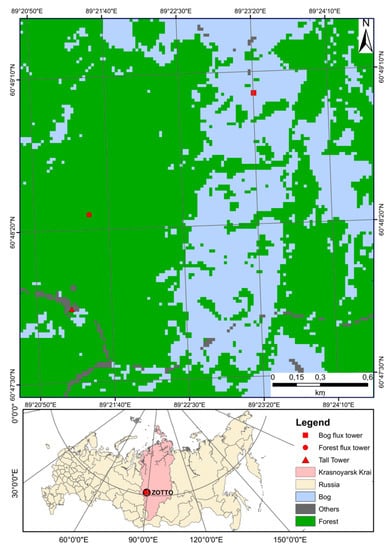
Figure 1.
Land-cover map and geographical locations of forest (ZF; red circle) and bog (ZB; red rectangle) flux towers and tall tower (red triangle) in Zotino, Krasnoyarsk Krai, Russia (black circle). The map is derived from 30 m resolution Landsat-8 image. The ZOTTO denotes the Zotino Tall Tower Observatory. We reclassified 14 initial land-cover types into 3 types. Forest includes reforestation, regrowth, and lichen with pines. Bog includes shrubs, flooded, and wet body. Other classes (others) include clear-cut/barren, burned, sand, and sparse vegetation.

Table 1.
Site characteristics of the forest and bog flux towers at Zotino.
The Zotino bog flux tower (hereafter ZB, 60°49′03″ N, 89°23′20″ E, 66 m a.s.l.) is situated approximately 2 km to the northeast of the ZOTTO. The average canopy height at the site was approximately 2.5 m, and the measurement height was 9.9 m (Table 1 and Figure 1). The type of peat is classified as an ombrotrophic [21]. The landscape was covered by a pine-dwarf, shrub-sphagnum (in Siberia, called ryam), hollow-ridge complex. They had a height of 0.4–0.6 m and were covered by plant communities consisting of dwarf pine (Pinus sylvestris f. litwinowii), which dominates the trees and dwarf shrubs (Chamaedaphne calyculata). The peat’s calibrated age at the bottom of the bog ranged from 9397 ± 134 y BP at the edges to 13617 ± 190 y BP at the bog’s center. The peat depth showed a wide range from 1.60 m to 5.10 m, increasing toward the bog’s center.
2.2. Measurement System
Identical micrometeorological measurement systems were installed at the forest and bog sites (Table 2). The EC system consisted of a three-dimensional ultrasonic anemometer (USA-1, Metek GmbH, Elmshorn, Germany) with integrated 55 W heating and closed-path infrared gas analyser (LI-7200, LiCor Biosciences, Lincoln, NE, USA) to measure CO2 and H2O fluxes at 20 Hz frequency. An external diaphragm vacuum pump transported air to the gas analyser with a flow rate of 13 L min−1 at ambient atmospheric pressure. At the top of the towers, sensors measured the four radiation components and photosynthetically active radiation (PAR), air temperature (Ta), relative humidity, and atmospheric pressure. Soil or peat temperature (Ts) was measured by PT100 soil-temperature probes at six depths (0.02, 0.04, 0.08, 0.16, 0.32, and 0.64 m for forest and 0.04, 0.08, 0.16, 0.32, 0.64, and 1.28 m for bog, respectively). Soil moisture was measured by six sensors at both sites: two sensors at 0.08 m and one sensor at each depth of 0.16, 0.32, 0.64, and 1.28 m at the ZF and six sensors at a depth of 0.08 m at the ZB. Data collected from the EC system and meteorological measurements were stored on a data logger (CR3000, Campbell Scientific Inc., Logan, UT, USA). Details in setup of the EC system have been described by Park et al. [42]. Snow depths at both sites were measured manually at locations nearby the towers; however, the measurement intervals were irregular.
Table 2.
Instrument setup and sensor types of the flux towers at the Zotino sites.
2.3. Post-Processing of Data and Quality Control
We applied the data processing scheme for the closed-path analysers mentioned in Mammarella et al. [45]. In the raw data post-processing step, spike detection, 2D coordinate rotation, and time lag adjustment as well as calculation of half-hourly turbulent fluxes were performed using the EddyUH software [45]. The thresholds of friction velocity (u*) for ZF and ZB were 0.2 m s−1 and 0.1 m s−1, respectively. Details of the post-processing steps and quality control have been described by Park et al. [42]. The high-quality data available after the quality check and u* filtering led to a data coverage of 42–61% for ZF and 19–51% for ZB for 2013–2017. To calculate the cumulative CO2 flux (NEEcum), we gap-filled the half-hourly data using the REddyProc [46] in R [47]. Storage flux calculation was applied only for ZF data.
2.4. Data Anlaysis and Statistical Model
In this study, ‘spring’ is defined from the day of year (DOY) of 91–165 (01.04–14.06), 2013–2017. Daily CO2 fluxes were summed for each 24-h period with gap-filled data. Regarding the EC convention, a negative NEE or CO2 flux refers to net CO2 uptake by the ecosystem, whereas a positive NEE indicates CO2 release from the ecosystems to the atmosphere.
We used surface albedo (Alb) as a proxy for the status of snowmelt, as suggested in previous studies [22]. We determined the final day of snowmelt on which the 3-day moving average of Alb fell below 0.15 (15%) for the first time. To detect the final day of snowmelt, Shibistova et al. [28] used the daily mean soil temperature at a depth of 0.05 m and a 15-day moving average as the final day of snowmelt; however, in the present study, we used diurnal patterns of surface or peat temperature at a depth of 0.04 (Ts04). To examine the effect of temperature accumulation on vegetation productivity, we defined the accumulated growing degree days for air temperature (CGDDTa) and surface soil or peat temperature (CGDDTs04). We computed the cumulative sums of daily mean Ta and Ts04 above 0 °C (base temperature 0 °C) from DOY 99–165.
To identify the abiotic variables that are important in explaining the variability in daily CO2 flux, we used the multivariate adaptive regression splines (MARS) regression model [48], specifically, the earth package [49] in R [47]. Daily CO2 fluxes with corresponding abiotic variables were used as training data for both sites from DOY of 99 to 165 in 2013–2017 for ZF and the same days in 2014–2016 for ZB, respectively. Several previous studies have shown that spring CO2 uptake is associated with four environmental factors: air temperature (Ta), Ts04, beginning day of snowmelt, and final day of snowmelt [21,22,23,24]. Therefore, we included Ta, Ts04, and Alb to construct the MARS model. For ZF, we used nine abiotic variables as training data: PAR, Alb, Ta, midday vapour pressure deficit (VPD), Ts04, and soil or peat temperature at depths of 0.08 m (Ts08), 0.16 m (Ts16), 0.32 m (Ts32), and 0.64 m (Ts64). For ZB, a total of seven abiotic variables were used as training data: the same as those for ZF but excluding Ts08 and Ts16 due to the long-term data gaps (>3 months) in the data for these two variables.
The MARS is a non-parametric regression method that can deal with both linear and nonlinear relationships and interactions between variables in the data using hinge functions [48]. Variable selection algorithms search the variables using both forward and backward stepwise selections. Variable importance is determined by a selection algorithm and is based on the number of model subsets (nsubsets), generalized-cross validation (GCV) score, and residual sum of squares (RSS). The GCV and RSS were scaled from 0 to 100. Higher GCV scores indicate variables with more explanatory power. The largest summed decrease of the RSS is scaled to 100, meaning that a large net decrease in the RSS is more important than a low RSS. Higher nsubsets means that variables are included in more subsets because they are important. Further statistical theory and application are described in detail at http://www.milbo.org/doc/earth-notes.pdf (accessed on 26 July 2021).
To investigate the impacts of cold spring weathers on the net ecosystem productivity (NEP), we used a rectangular hyperbolic light-response functional relationship [50] between PAR and NEP. We examined the differences in curve shapes and fit parameters for the year with the most frequent cold spring weather days (2014) and the year with the least frequent cold spring weather days (2015) with the following Equation (1):
where PAR (µmol photon m−2 s−1) is the incident photosynthetically active radiation, Amax (µmol CO2 m−2 s−1) is the light-saturation point of CO2 uptake, and α is the initial slope of the NEP-PAR (net CO2 uptake at light saturation), and Rd is the ecosystem respiration during the day (µmol CO2 m−2 s−1). We used daytime data for which potential global radiation (Rpot) exceeded 20 W m−2. To make it easier to visualize, we used NEP, which is opposite in sign to NEE. Three model parameters were estimated for the selected two periods estimated using the Levenberg–Marquardt method, implemented in the minpack.lm package [51] in R [47]. The Levenberg–Marquardt method is a widely used algorithm for analyzing non-linear light-response curves [52,53]. NEPsat was calculated with the obtained three parameters and by fixing PAR at 1500 µmol photon m−2 s−1. The definition of NEPsat was the similar concept addressed by Migliavacca et al. [52] and Musavi et al. [54]. NEPsat helps to understand NEP at light saturation when PAR as 1500 µmol photon m−2 s−1 corresponds to light saturation.
3. Results
3.1. Abiotic Controls of Spring CO2 Fluxes
Temporal evolutions of daily CO2 fluxes and associated abiotic drivers in 2016 showed that CO2 flux variations generally corresponded to the rapid increasing Ta and Ts04 after snowmelt had completed (Figure 2). We confirmed that these highly fluctuating features of fluxes and spring meteorological conditions were similar in other years (Supplementary Figure S1). CO2 fluxes at ZF increased faster than at ZB after snowmelt. Similar features were observed in other years. Alb at ZB was remarkedly different from that at ZF because of the higher radiation absorption by forest. Sporadic warm spells temporarily led to a rapid net uptake of CO2 at ZF. In contrast, net CO2 uptake rates at ZB did not increase as rapidly as those at ZF because the Sphagnum peat was still under snow cover and therefore less affected by changes in Ta. During the snowmelt period (DOY 127–145), the forest transitioned from a net CO2 source to a net CO2 sink. However, CO2 fluxes were still highly variable during this time, fluctuating between net CO2 source and net CO2 sink.
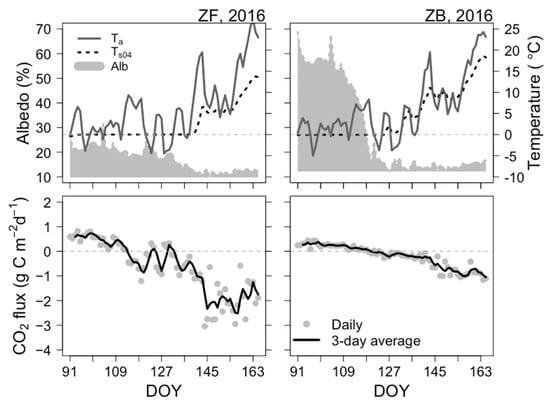
Figure 2.
Time-series of three major environmental drivers and CO2 flux for the period DOY 91–165 in 2016 at ZF and ZB sites. Upper panel: daily mean air temperature (Ta, dark-grey line; unit: °C), soil/peat temperature at 0.04 m (Ts04, dotted black line; unit: °C), and albedo (Alb, grey-shaded area; unitless). Lower panel: daily net CO2 flux (grey circle; unit: g C m−2 d−1) and 3-day moving average CO2 flux (black line; unit: g C m−2 d−1). The dashed grey line denotes the zero-line of CO2 flux, with positive CO2 flux values indicating a net CO2 source and negative values indicating a net CO2 sink.
In a typical springtime, Ta was highly variable, ranging from −5 °C in April to 25 °C in May (Figure 2). The amplitude of Ta was ~30 °C, which is typical of boreal spring weather. At the end of the snowmelt stage, the increase in Ta was considerable (by ~15 °C). This may have led to the disappearance of snow cover on the ground surface, resulting in the observed increase in Ts04 during this period to above 5 °C. As shown in Figure 2, we also confirmed that Ts04 at ZB increased above 15 °C, which was ~5 °C warmer than at ZF for every spring in the study period (Supplementary Figure S1).
At both ecosystems, the start of net CO2 uptake occurred during periods with cold or frozen soil (Figure 2). However, the magnitude of daily CO2 uptake was lower than −1 g C m−2 d−1 until thawing of the surface soil (Ts04 < 0 °C) or snowmelt was complete. CO2 uptake rates remained almost neutral and constituted a net CO2 sink only when Ts04 recovered above 0 °C (DOY 120). As shown in Figure 2, data for both sites reveal that the transition from net CO2 source to net CO2 sink can be disrupted temporarily by cold spells (DOY 110–135). This feature was more distinct in forest ecosystem.
In 2016, the transition from net CO2 source to net CO2 sink occurred earlier in the forest than in the bog (Figure 2). Although the soil was still frozen, if the temperature was favourable (~5 °C) for photosynthesis, the forest ecosystem transformed into a weak net CO2 sink. For instance, the start of net CO2 uptake at ZF was on DOY 114 in 2016. Mean Ta from DOY 113 to 119 was 7.7 °C, which favoured the triggering of the start of net CO2 uptake. Compared with ZF, ZB was a not yet an active CO2 sink, probably because the ground layer peat mosses were partially covered by snow.
We used the MARS model to examine the relative importance of factors controlling CO2 fluxes over the study period. The fitting of this model showed fairly good predictive performance (84–89%; Table 3). For ZF, the MARS model identified six variables (Ts04, PAR, Alb, Ta, Ts16, and Ts64) as the important influences on CO2 fluxes out of the nine analysed. The percentage of variance in daily CO2 fluxes explained by the model (R2) was 84%. For ZB, the MARS model identified five variables (Ts04, Alb, Ts64, PAR, and Ts32) as the important influences on CO2 fluxes out of the seven variables analysed, with R2 of 89% at ZB. Although we did not use ecological model, results show that the MARS model captured the controlling factors of CO2 fluxes fairly well by considering non-linear relationships between modelled CO2 fluxes and abiotic drivers.
Table 3.
The order of important variables with statistics (nsubsets, GCV, and RSS; see details in Section 2.4) of CO2 flux estimated by using the MARS model in spring period (DOY 99–DOY 155) from 2013 to 2017 at the ZF and ZB sites. For ZF, a total of 285 daily means of variables (Ta, Ts04, Ts08, Ts16, Ts32, Ts64, Alb, PAR, and VPD) were used as initial data. The percentage of variance in daily CO2 fluxes explained by the model (R2) was 84%. For ZB, a total of 216 daily means of variables were used for the period DOY 111–155 in 2013 and DOY 99–115 in 2014–2016. Peat temperatures at depths of 0.08 and 0.15 m were excluded for the initial data of the MARS model due to the long-term data gaps (>3 months) for 2014–2015. The percentage of variance in daily CO2 fluxes explained by the model (R2) was 89%.
3.2. Impacts of Cold Weather on Photosynthesis-Related Parameters
During the springtime, Ta was highly variable, with several apparent cold and warm phases (Figure 2). To examine the overall impacts of cold weather on CO2 fluxes, we compared the photosynthesis-related parameters between the year having the most frequent cold spring weather days (2014) and the year having the least frequent cold spring weather days (2015) using the PAR-NEP relationship (Figure 3 and Table 4). Here, we defined cold spring weather as the day with a minimum daily Ta < 0 °C. For both sites, 2014 had the most frequent cold weather days (13 days for ZF and 15 days for ZB), and 2015 had the least frequent cold weather days (0 days for ZF and 2 days for ZB) compared with the entire study period (6 days for ZF and 10 days for ZB, 5-year mean values).
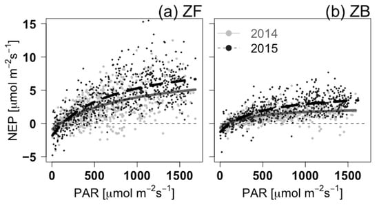
Figure 3.
Ecosystem light-response curves for the year with the highest frequency of cold weather days (2014, grey dots and dark-grey lines) and the year with the lowest frequency of cold weather days (2015, black dots and dashed black lines) for (a) ZF and (b) ZB. Half-hourly daytime (potential global radiation > 20 W m−2) data were chosen for after snowmelt (DOY 129–151 in 2014 and DOY 134–151 in 2015 for ZF; DOY 125–151 in 2014 and DOY 132–151 in 2015 for ZB). Fit parameters and statistics are listed in Table 4.
Table 4.
Model parameters of the rectangular light-response function for the year with the most frequent cold weather days (2014) and for the year with the least frequent cold weather days (2015) for both ZF and ZB. Numbers in parentheses denote the standard errors of the parameters. n is the number of half-hourly data. As NEPsat is a function of Amax, , Rd, and PAR at saturation PAR of 1500 mol photon m−2 s−1, the standard deviations of NEPsat were taken as the averaged maximum and minimum standard errors of each parameter.
It is a typical feature that half-hourly CO2 fluxes during spring daytime are highly scattered due to large temperature changes or cloud cover (Figure 3). Nevertheless, the light-response curves of both ecosystems showed typical shapes of rectangular hyperbola curve. The curve showed a rapid and linear increase in NEP at lower PAR levels, with a slow increase to reach maximum NEP at high PAR levels (Figure 3). Bogs fixed CO2 at much lower PAR levels compared with forests. Under the same environmental conditions, for instance, needle-leaves at the top of the forest canopy are likely to warm sufficiently to photosynthesise compared with the understory vegetation, such as that found at the bog site. Due to the wider range of NEP for forest than those for bog, residual standard errors for ZF were larger than those for ZB (Table 4). Mean Ta values after snowmelt in 2014 and 2015 were ~5 °C and ~13.5 °C, respectively. As a result, both ecosystems seem to have higher Amax and NEPsat in 2015 than in 2014. Amax from the rectangular hyperbola photosynthetic light-response function had a higher light saturation level than the one from the non-rectangular hyperbola curve because the latter had a stronger flattening at the light-compensation point. Therefore, NEPsat better represents values of the maximum CO2 uptake rate of ecosystems. Compared with the bog, the forest had approximately three times higher Amax and NEPsat.
Quantum yields (α) at both ecosystems were similar in 2014 and increased by more than 50% in 2015 (Table 4). In this period, the light-response curves for ZB reached at light-saturation point earlier than for ZF, indicating that the bog reached its maximum ability to fix CO2 earlier than for the forest due to lower light-use efficiency (Figure 3). Interestingly, the relative changes in NEPsat of ZF and ZB in 2015 were approximately +32% and 74%, respectively. Presumably, the contribution of soil microbes in the ecosystem respiration term under the warm spring in 2015 may be greater than in 2014.
3.3. Interannual Variability of Spring Cumulative NEEcum
Overall variations in spring NEEcum were more distinct at ZF compared with ZB, as shown by daily CO2 fluxes in Figure 2. Spring NEEcum between 2014 to 2016 ranged from −27.6 to −37.2 g C m−2 at ZF and from −7.7 to −14.9 g C m−2 at ZB (Figure 4 and Table 5). Compared with the features at ZB, NEEcum at ZF showed larger amplitudes and higher uptake rates, which indicate that forest is a stronger spring CO2 sink than the bog. When thick snow depth rapidly decreased with increasing temperature, between DOY 120 and 130, 2014–2016, both ecosystems released CO2 in the atmosphere.
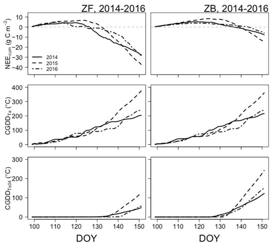
Figure 4.
Cumulative net ecosystem exchange of CO2 (NEEcum; g C m−2, top), cumulative growing degree days of daily mean air temperature (CGDDTa; °C, middle), and cumulative growing degree days of daily mean surface soil/peat temperature (CGDDTs04; °C, bottom) for ZF (left panel) and ZB (right panel). Solid, dashed, and long-dashed black lines denote data for DOY 99–155 for 2014, 2015, and 2016, respectively. Dashed grey zero-lines in the top panel denote the transition from a cumulative CO2 source (positive, ecosystem carbon loss) to cumulative CO2 sink (negative, ecosystem carbon gain).
Table 5.
Cumulative net ecosystem exchange of CO2 (NEEcum; g C m−2), the day of year (DOY) of transition from NEEcum source to NEEcum sink (NEEcum,tran; DOY), cumulative growing degree days of air temperature (CGDDTa; °C) corresponding to NEEcum,tran, cumulative growing degree days of surface soil temperature (CGDDT04; °C) corresponding to NEEcum,tran, and mean slope (; g C m−2 d−2) after reading peak of NEEcum for ZF and ZB for the period DOY 99–155 in 2014–2016.
To compare the rate of change of interannual variability in NEEcum, the mean slopes of the curve () following peak NEEcum were examined (Table 5). Both ecosystems showed steeper declining slopes after the peak of NEEcum in the three years studied, particularly the steepest in the warmest year (2015); was −1.62 g C m−2 d−2 for ZF and −0.92 g C m−2 d−2 for ZB. For both ecosystems, 2015 was the year with the largest NEEcum for both the 3-year period (2014–2016) and the entire study period. In 2015, Ta in May was ~10 °C, which was 4.2 °C higher than the 5-year mean (5.8 °C) (Figure 5). For both ecosystems, NEEcum was strong and negatively correlated with mean Ta in May (R2 = 0.69, P = 0.081 for ZF and R2 = 0.79, P = 0.110 for ZB). Unusually high mean Ta in May corresponded to the highest NEEcum, meaning that the ecosystems were the strongest CO2 sinks in the warmest year.
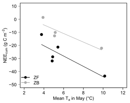
Figure 5.
Relationships between cumulative NEE (NEEcum; g C m−2) and mean Ta in May (°C) from 2013 to 2017 for the ZF and ZB sites. Linear regression for ZF (black dot and line): NEEcum = −4.52*Ta − 3.94, R2 = 0.69, P = 0.081; linear regression for ZB (grey dot and line): 8.77*Ta − 3.28, R2 = 0.79, P = 0.110. NEEcum was calculated from DOY 110–155 in 2013 only for ZB, and the rest of other years for both sites were calculated from DOY 99–155.
Rapid increasing trends in accumulated growing degree days of air and soil temperatures were followed by the steep decreasing slope in NEEcum,tran. These characteristics showed similar variations and trends over the three years. For instance, in 2014, transition day (DOY) from NEEcum source to NEEcum sink (NEEcum,tran) at ZF was DOY 128, corresponding to CGDDTa at 104.5 °C. At this point, Ts04 was positive but stayed close to 0 °C. This implies that Ta plays an important role in NEEcum transition time, as we observed in Figure 2. Before surface Ts04 stays nearly 0 °C, the forest was net CO2 source. Rapid increasing phase in NEEcum followed a steep and a linear increase of CGDDT04 > 4 °C. CGDDT04 increased more than 7 °C in two days (DOY 135–137). After DOY 136, the slope of NEEcum/DOY was −1.05 g C m−2 d−2. From this point, ZF entered the growing season, and photosynthesis had fully recovered from the cold season. Both photosynthesis and ecosystem respiration continuously increase over the growing season. At ZB, NEEcum,tran was 10 days later (DOY 138) than the NEEcum,tran at ZF. At this time, peats were already warmed up, showing positive temperatures (CGDDTa = 164.6 °C). Similar to forest, daily mean Ts04 also increased approximately 7 °C in two days (DOY 128–130) immediately after CGDDT04 exceeded 1 °C. Presumably, the ground surface at ZF is still partly covered by snow, and shading by trees may result in warmer surface conditions later than at ZB. If mosses were exposed to the open space without shading, then they could receive more direct solar radiation on the surface, which may result in earlier soil warm-up conditions. Characteristics of NEEcum,tran and heat accumulation explained by CGDDTa and CGDDT04 imply that the bog seems to have a higher level of temperature accumulation than forest, because soil microbial activity requires a suitable temperature level, corresponding to daily Ts04 > ~7 °C and CGDDT04 of ~41 °C.
In 2015, NEEcum,tran at ZF occurred in DOY 134, corresponding to CGDDTa at 137.6 °C. Although the spring mean Ta in 2015 was the highest, NEEcum,tran in 2015 occurred the latest compared with other years. Perhaps, warm temperature conditions increase ecosystem respiration, leading to the forest remaining a net CO2 source for longer. To find a reasonable answer, we will intend to examine components of the flux partitioning for a future study. Anomalously high Ta also led to the highest Ts04. CGDDTa during DOY 100–150 matched with the transition point of CGDDT04 > ~4 °C. Compared with ZF, CGDDT04 corresponding to NEEcum,tran at ZB varied 40–75 °C. CGDDT04 at ZB showed more rapid enhancement in other years, possibly associated with the soil microbial responses to warm temperature conditions.
4. Discussion
4.1. Identifying the Major Drivers of CO2 Fluxes
At our sites, spring CO2 fluxes were mainly controlled by air temperature (Table 2). A rapid rise in CO2 uptake occurred after surface snow melted, and Ts04 warmed above 1 °C (Figure 2). We confirmed that abiotic controlling factors of CO2 fluxes identified from the MARS model agreed with previous findings. In boreal coniferous forests, spring photosynthesis recovery is related to air temperature, surface soil temperatures, first day of snowmelt, and final day of snowmelt [20,22,23,24,25,26,29]. The coniferous forest was already a net CO2 sink before the end of snowmelt and while part of the soil surface was still frozen (Figure 2). In a wider context, this result agrees with the finding of Parazoo et al. [55], who showed that spring thaw was the crucial trigger for the start of spring photosynthesis and net CO2 uptake in boreal forests in Arctic ecosystem. In northern peatland, peat temperature and snowmelt completion have been shown to affect the rapid increase in vegetation productivity [11,18,21,25]. In addition, PAR and temperature have been identified as controlling factors on the CO2 flux of peat during the growing season [26,56,57].
In our study, Ts04 was identified as the primary driver of CO2 fluxes for both ecosystems (Table 2). From a biophysical point of view, light (i.e., PAR) is known to be the primary driver of the beginning of net CO2 sink or photosynthesis. In a previous study, a data-driven approach similar to the one used here identified PAR as the most important driver of CO2 fluxes at the ZF site [42]. During the growing season, including the snow-melting period, PAR strongly controls the growth of Sphagnum [57]. In the boreal winter-to-spring transition period, snow cover decreases as temperature rises, as shown in reverse patterns of surface reflectance and air temperature [21,22,23]. This reflects that, in reality, Ts04 and Alb are indirect drivers of CO2 fluxes.
We chose the MARS model to identify the relative importance of controlling factors of CO2 fluxes because of its simplicity. In our study site, we often met a long-term data gap, particularly in the winter and early season, meaning that estimates of a reliable annual carbon budget with uncertainty are challenging. To overcome this limitation, further efforts for utilizing major variables identified from the MARS model and/or incorporating with other machine-learning methods suitable for a relatively smaller dataset (e.g., support vector machine) are desirable. With such efforts, we can develop an advanced version for the site-specific gap-filling algorithm.
4.2. Potential Drivers of Spring CO2 Fluxes
We observed that Ta, Ts04, Alb, and PAR affect seasonal variations of CO2 fluxes at a boreal forest and a bog. However, there is still room for exploring unknown or missing drivers of spring CO2 fluxes. For instance, a recent study by Koebsch et al. [58] suggested that biological drivers seem more important for determining the variability in maximum gross primary productivity compared with abiotic drivers in boreal peatlands. Peichl et al. [59] also emphasized the important role of phenology on seasonal variation of photosynthesis in European peatlands. In addition, it is likely that the rapid increase in net CO2 uptake after the snowmelt completion at ZB (Figure 2) may be associated with increases in peat temperatures in the rooting zone (0.1–0.2 m), leaf nitrogen, and chlorophyll a concentration [25]. This suggests that chlorophyll a could be a potential biochemical driver of spring CO2 fluxes in peatlands.
In peatland, hydrological drivers (e.g., precipitation, soil moisture, and water-table depth) and their regime are also crucial for understanding photosynthesis-related processes. Previous studies [11,60,61] suggest that the water-table depth is an important control on the growing season NEE and the annual CO2 balance, although this control appears to be site dependent. In contrast to previous studies, Strachan et al. [62] did not find significant relationships between peatland productivity or cumulative CO2 exchange and early season temperature, the timing of snowmelt, or growing season length at an ombrotrophic bog located in Canada. Our data was limited in analyzing the roles of hydrological factors on seasonality of CO2 uptake in peatland; thus further efforts to examine the roles of biotic and abiotic drivers in regulating peatland C cycle at ZB are desirable. In addition, measurement of other important components of C flux, such as methane, are necessary to better understand the annual C balance in peatland [1,17,63,64].
4.3. Role of Air and Soil Temperatures on Vegetation CO2 Uptake Capacity in Northern Eurasia
Consistent with characteristics of abiotic drivers of CO2 fluxes shown in Figure 2, NEEcum,tran at ZF requires suitable air temperature accumulation (CGDDTa > ~100 °C) more than soil temperature (Figure 4, Table 5). In previous studies, 5-day running mean of daily mean air temperature and cumulative temperature were good predictors of the commencement of spring photosynthesis in boreal coniferous forests [22,23].
We confirmed that both ecosystems have a zero-curtain period at Ts04 that remained close to 0 °C around until mid-April (Figure 2). This feature is a typical phenomenon in high-northern latitude or alpine ecosystems during the winter-to-spring transition period [21,23,25,60,65,66,67]. Although the surface snow may not have fully disappeared, warm spells may affect the timing of the start of net CO2 uptake in boreal forests (Figure 2). Such phenomena may be a piece of evidence that Scots pines growing in high latitudes have adapted to water-limited environments in severe and long winters. Generally, low soil-temperature conditions during spring constrain water uptake and root activity in boreal conifers [24,66,68,69]. However, there is observational evidence that pine trees in winter use stem-stored water regardless of snowmelt termination or available soil water to maintain their metabolism [22,70]. It is also possible that different tree species may have different strategies for the process of spring photosynthesis recovery [71].
Cold weather appears to temporarily reduce CO2 uptake rates over the study period. However, plants recovered CO2 uptake rates as soon as Ta increased above 0 °C (Figure 2). We found a similar pattern in other years (Supplementary Figure S1), which tend to be more distinct in the forest than in the bog. In addition, our data reveal that colder spring weather conditions resulted in a reduction of the maximum photosynthetic capacity (Figure 3). In previous studies, intermittent cold temperatures, for instance, frost events, delayed the photosynthesis recovery process of conifers, and the effect is more pronounced if frost is severe [20,72,73]. In peatlands, chilling can reduce chlorophyll a concentration [25,74]. It is unclear to find these features from daily CO2 fluxes in our study; however, Figure 3 and Table 4 seem to show clues; cold weather temporarily suppresses photosynthetic capacity during spring. Overall, our data showed reasonable ranges and PAR-NEP fit parameters compared with the previous study [64].
A warmer climate may result in an earlier start of spring photosynthesis and increased vegetative productivity as well as annual CO2 uptake in boreal coniferous forests [29,30,73]. However, the effect of warm temperatures on the net CO2 uptake capacity of peatlands is likely to be more complex than that of forests because of soil hydrological conditions. Precipitation, water table depth, vegetation type, and phenology are recognised as other important controls on CO2 fluxes, and their effects on net CO2 uptake seem to be highly site dependent [11,12,14,37,59].
In this study, both ecosystems showed the highest vegetation productivity in 2015 (Figure 5). Despite the small amount of data and highly deviated data in 2015, both ecosystems showed negative relationships between NEEcum and mean Ta in May. Based on the spatial distribution of 2m temperature anomalies over the study period (2013–2017), it is highly likely that vegetations in Zotino absorb the highest CO2 uptake among the years because of anomalously warm temperature in May (Supplementary Figure S2). Anomalous warm temperatures were spread over the western Siberia, including the Zotino site. A study by Alekseychik et al. [37] seems to support that our finding is possible. They reported that the spring in 2015 was warmer; monthly mean air temperature in May was 4.1 °C higher than the long-term average in a similar type of bog in Finland. Besides, Liu et al. [14] and Pulliainen et al. [29] found that net CO2 uptake in boreal ecosystem during the warm spring was greater than the normal year, implying that vegetation is sensitive to the changes in air temperature, and it is a crucial driver to understand spring C uptake. To obtain the robust relationship between NEEcum and mean Ta in May, we plan to analyze the longer term of vegetation indices using remote sensing data together with flux data. In addition, Alekseychik et al. [37] also found that despite the very warm spring in 2015, cloudy and rainy weather conditions in summer in that year resulted in a lower CO2 uptake for the growing season compared with other years. This implies that the high vegetation productivity induced by the anomalously warm temperatures in May 2015 is likely to have been compensated by the cool and wet ensuing summer. Our forthcoming research will examine the annual net CO2 balance through comparison of the results of the present study with those from other sites in Siberia and for different weather conditions.
5. Conclusions
CO2 flux observations at the Zotino sites showed that distinct differences exist in flux magnitude, the timing of start of net CO2 uptake, and the rate of CO2 uptake between the boreal forest and bog. In spring, the boreal forest generally changed from net CO2 source to net CO2 sink approximately 1–2 weeks earlier than the bog. We found similar aspects for the transition from NEEcum source to NEEcum sink. Rapid net CO2 uptakes for both ecosystems covaried with Ta, corresponding to Ts04 values > 5 °C. To change into complete NEEcum sink, ZF seems to require CGDDTa of ~80 to 137 °C and ZB requires CGDDTa of 141 to 211 °C. Compared with ZF, seasonal variations in NEE-cum at ZB were smaller. This implies that forests appear more sensitive to the changes in air temperature than bogs under the same spring weather conditions. We confirmed that cold spring weather reduced the maximum photosynthetic capacity in both ecosystems. During the study period, abnormally warm air temperatures in spring 2015 resulted in the highest vegetation productivity. Overall, results suggest that the CO2 uptake capacities of boreal forest and bog are sensitive to rising air temperature in springtime. This strong relationship between air temperature and NEE seems to support that a linear relationship between NEE estimated from the atmospheric inversion method and air temperature proposed by Rödenbeck et al. [75].
Our analysis is limited in analyzing NEE; thus, future work will examine the effects of anomalously warm spring weather on both photosynthesis and respiration with respect to the annual C balance. Besides, we will investigate the linkage between hydrological conditions (e.g., snow depth and rainfall) in the previous winter and seasonal/annual CO2 balances in the following year. To overcome the limited number of EC flux measurement, remote-sensing-based phenology and photosynthesis products will be utilized. We anticipate direct CO2 flux measurements at Zotino will be valuable for evaluating biogeochemical models. Further, it will provide insights into the prediction for the future terrestrial C cycle in northern Eurasia, particularly in remote and relatively undisturbed natural ecosystems.
Supplementary Materials
The following are available online at https://www.mdpi.com/article/10.3390/atmos12080984/s1, Figure S1: Same as Figure 2, but for (a) 2013, (b) 2014, (c) 2015, (d) 2017 at ZF and ZB. No available CO2 flux measurements at ZB in 2017, Figure S2: Spatial distribution of 2 m temperature anomalies in May for each year over the 5-year mean (May, 2013–2017) from Climate Reanalyzer (https://ClimateReanalyzer.org, accessed on 17 July, 2021), Climate Change Institute, University of Maine, USA. ERA5 is the fifth generation ECMWF atmospheric reanalysis data produced by the Copernicus Climate Change Service (C3S). The spatial resolution of ERA5 is at 0.5°. ZOTTO is situated approximately at 60°N, 89°E. 2m temperature anomaly for (a) May 2013, (b) May 2014, (c) May 2015, (d) May 2016, and (e) May 2017, respectively.
Author Contributions
Conceptualization, S.-B.P., A.K., and M.M.; methodology, S.-B.P., M.M., T.T., I.M., O.P. and A.P.; software, S.-B.P. and O.K.; validation, S.-B.P. and O.K.; investigation, S.-B.P., A.K. and M.M.; resources, T.V.; writing—original draft preparation, S.-B.P.; visualization, S.-B.P.; supervision, A.K.; funding acquisition, J.L., M.H. and S.S.P. All authors have read and agreed to the published version of the manuscript.
Funding
The ZOTTO project is funded by the Max Planck Society through the International Science and Technology Center (ISTC) partner project no. 2757 within the framework of the proposal “Observing and Understanding Biogeochemical Responses to Rapid Climate Changes in Eurasia”. S.-B.P. and S.S.P. are supported by National Research Foundation of Korea (NRF- 2020R1C1C1013628). A.P. is supported by grant RFBR #18-05-60203-Arktika. T.V. thanks the grant of the Tyumen region, Russia, Government in accordance with the Program of the World-Class West Siberian Interregional Scientific and Educational Center (National Project “Nauka”).
Institutional Review Board Statement
Not applicable.
Informed Consent Statement
Not applicable.
Data Availability Statement
Data are available upon reasonable request to the corresponding author.
Acknowledgments
S.-B.P. acknowledges the International Max Planck Research School for Global Biogeochemical Cycles (IMPRS-gBGC). We deeply thank the technical staff for maintaining the eddy covariance flux towers: Karl Kübler, Steffen Schmidt, and Martin Hertel from the Freiland group, Max Planck Institute for Biogeochemistry in Jena; Alexey Panov, Alexander Zukanov, Nikita Sidenko, Sergey Titov, and Anastasiya Urban from the V.N. Sukachev Institute of Forest in Krasnoyarsk; and many other supporters in Zotino. S.-B.P. thanks to colleagues at the MPI-BGC; Andrew Durso, Kendalynn Morris, Jeffrey Beem-Miller, and Shane Stoner for proofreading on the manuscript; Talie Musavi for advising statistical analysis; and Marcus Guderle for creating Figure 1. Authors are grateful to three anonymous reviewers for their helpful comments and suggestions for improvements of the manuscript.
Conflicts of Interest
The authors declare no conflict of interest.
References
- Schulze, E.D.; Lapshina, E.; Filippov, I.; Kuhlmann, I.; Mollicone, D. Carbon dynamics in boreal peatlands of the Yenisey region, western Siberia. Biogeosciences 2015, 12, 7057–7070. [Google Scholar] [CrossRef] [Green Version]
- Dolman, A.; Shvidenko, A.; Schepaschenko, D.; Ciais, P.; Tchebakova, N.; Chen, T.; van der Molen, M.; Marchesini, L.B.; Maximov, T.C.; Maksyutov, S.; et al. An estimate of the terrestrial carbon budget of Russia using inventory-based, eddy covariance and inversion methods. Biogeosciences 2012, 9, 5323–5340. [Google Scholar] [CrossRef] [Green Version]
- Gorham, E. Northern Peatlands: Role in the Carbon Cycle and Probable Responses to Climatic Warming. Ecol. Appl. 1991, 1, 182–195. [Google Scholar] [CrossRef] [PubMed]
- Smith, N.V.; Saatchi, S.S.; Randerson, J.T. Trends in high northern latitude soil freeze and thaw cycles from 1988 to 2002. J. Geophys. Res. Space Phys. 2004, 109, 1–14. [Google Scholar] [CrossRef]
- Luyssaert, S.; Inglima, I.; Jung, M.; Richardson, A.D.; Reichstein, M.; Papale, D.; Piao, S.L.; Schulze, E.-D.; Wingate, L.; Matteucci, G.; et al. CO2 balance of boreal, temperate, and tropical forests derived from a global database. Glob. Chang. Biol. 2007, 13, 2509–2537. [Google Scholar] [CrossRef] [Green Version]
- Yu, Z.C. Northern peatland carbon stocks and dynamics: A review. Biogeosciences 2012, 9, 4071–4085. [Google Scholar] [CrossRef] [Green Version]
- Minkkinen, K.; Ojanen, P.; Penttilä, T.; Aurela, M.; Laurila, T.; Tuovinen, J.-P.; Lohila, A. Persistent carbon sink at a boreal drained bog forest. Biogeosciences 2018, 15, 3603–3624. [Google Scholar] [CrossRef] [Green Version]
- Pan, Y.; Birdsey, R.A.; Fang, J.; Houghton, R.; Kauppi, P.E.; Kurz, W.; Phillips, O.; Shvidenko, A.; Lewis, S.; Canadell, J.; et al. A Large and Persistent Carbon Sink in the World’s Forests. Science 2011, 333, 988–993. [Google Scholar] [CrossRef] [Green Version]
- Lindroth, A.; Grelle, A.; Morén, A. Long-term measurements of boreal forest carbon balance reveal large temperature sensitivity. Glob. Chang. Biol. 1998, 4, 443–450. [Google Scholar] [CrossRef]
- Coursolle, C.; Margolis, H.; Giasson, M.-A.; Bernier, P.-Y.; Amiro, B.; Arain, M.; Barr, A.; Black, T.; Goulden, M.; McCaughey, J.; et al. Influence of stand age on the magnitude and seasonality of carbon fluxes in Canadian forests. Agric. For. Meteorol. 2012, 165, 136–148. [Google Scholar] [CrossRef] [Green Version]
- Bubier, J.L.; Crill, P.M.; Moore, T.R.; Savage, K.; Varner, R.K. Seasonal patterns and controls on net ecosystem CO2 exchange in a boreal peatland complex. Glob. Biogeochem. Cycles 1998, 12, 703–714. [Google Scholar] [CrossRef] [Green Version]
- Korrensalo, A.; Mehtätalo, L.; Alekseychik, P.; Uljas, S.; Mammarella, I.; Vesala, T.; Tuittila, E.-S. Varying Vegetation Composition, Respiration and Photosynthesis Decrease Temporal Variability of the CO2 Sink in a Boreal Bog. Ecosystems 2019, 23, 842–858. [Google Scholar] [CrossRef] [Green Version]
- Dorrepaal, E.; Aerts, R.; Cornelissen, J.H.C.; Callaghan, T.V.; van Logtestijn, R. Summer warming and increased winter snow cover affect Sphagnum fuscum growth, structure and production in a sub-arctic bog. Glob. Chang. Biol. 2003, 10, 93–104. [Google Scholar] [CrossRef]
- Liu, Z.; Kimball, J.S.; Parazoo, N.C.; Ballantyne, A.P.; Wang, W.J.; Madani, N.; Pan, C.G.; Watts, J.D.; Reichle, R.H.; Sonnentag, O.; et al. Increased high-latitude photosynthetic carbon gain offset by respiration carbon loss during an anomalous warm winter to spring transition. Glob. Chang. Biol. 2019, 26, 682–696. [Google Scholar] [CrossRef] [PubMed]
- Lloyd, J.; Shibistova, O.; Zolotoukhine, D.; Kolle, O.; Arneth, A.; Wirth, C.; Styles, J.M.; Tchebakova, N.M.; Schulze, E.-D. Seasonal and annual variations in the photosynthetic productivity and carbon balance of a central Siberian pine forest. Tellus B Chem. Phys. Meteorol. 2002, 54, 590–610. [Google Scholar] [CrossRef]
- Arneth, A.; Kurbatova, J.; Kolle, O.; Shibistova, O.B.; Lloyd, J.; Vygodskaya, N.N.; Schulze, E.-D. Comparative ecosystem-atmosphere exchange of energy and mass in a European Russian and a central Siberian bog II. Interseasonal and interannual variability of CO2 fluxes. Tellus B Chem. Phys. Meteorol. 2002, 54, 514–530. [Google Scholar] [CrossRef]
- Lund, M.; LaFleur, P.M.; Roulet, N.; Lindroth, A.; Christensen, T.; Aurela, M.; Chojnicki, B.; Flanagan, L.; Humphreys, E.; Laurila, T.; et al. Variability in exchange of CO2 across 12 northern peatland and tundra sites. Glob. Chang. Biol. 2009, 16, 2436–2448. [Google Scholar] [CrossRef]
- LaFleur, P.M.; Roulet, N.; Admiral, S.W. Annual cycle of CO2 exchange at a bog peatland. J. Geophys. Res. Space Phys. 2001, 106, 3071–3081. [Google Scholar] [CrossRef]
- Ottander, C.; Campbell, D.; Oquist, G. Seasonal changes in photosystem-II organization and pigment composition in Pinus sylvestris. Planta 1995, 197, 176–183. [Google Scholar] [CrossRef]
- Ensminger, I.; Sveshnikov, D.; Campbell, D.; Funk, C.; Jansson, S.; Lloyd, J.; Shibistova, O.; Öquist, G. Intermittent low temperatures constrain spring recovery of photosynthesis in boreal Scots pine forests. Glob. Chang. Biol. 2004, 10, 995–1008. [Google Scholar] [CrossRef]
- Arneth, A.; Lloyd, J.; Shibistova, O.; Sogachev, A.; Kolle, O. Spring in the boreal environment: Observations on pre- and post-melt energy and CO2 fluxes in two central Siberian ecosystems. Boreal Environ. Res. 2006, 11, 311–328. [Google Scholar]
- Thum, T.; Aalto, T.; Laurila, T.; Aurela, M.; Hatakka, J.; Lindroth, A.; Vesala, T. Spring initiation and autumn cessation of boreal coniferous forest CO2 exchange assessed by meteorological and biological variables. Tellus B Chem. Phys. Meteorol. 2009, 61, 701–717. [Google Scholar] [CrossRef] [Green Version]
- Tanja, S.; Berninger, F.; Vesala, T.; Markkanen, T.; Hari, P.; Mäkelä, A.; Ilvesniemi, H.; Hänninen, H.; Nikinmaa, E.; Huttula, T.; et al. Air temperature triggers the recovery of evergreen boreal forest photosynthesis in spring. Glob. Chang. Biol. 2003, 9, 1410–1426. [Google Scholar] [CrossRef]
- Suni, T.; Berninger, F.; Markkanen, T.; Keronen, P.; Rannik, Ü.; Vesala, T. Interannual variability and timing of growing-season CO2 exchange in a boreal forest. J. Geophys. Res. Atmospheres. 2003, 108, 4265. [Google Scholar] [CrossRef]
- Moore, T.R.; LaFleur, P.M.; Poon, D.M.I.; Heumann, B.W.; Seaquist, J.; Roulet, N. Spring photosynthesis in a cool temperate bog. Glob. Chang. Biol. 2006, 12, 2323–2335. [Google Scholar] [CrossRef]
- Frolking, S.E.; Bubier, J.L.; Moore, T.R.; Ball, T.; Bellisario, L.M.; Bhardwaj, A.; Carroll, P.; Crill, P.; LaFleur, P.M.; McCaughey, J.H.; et al. Relationship between ecosystem productivity and photosynthetically active radiation for northern peatlands. Glob. Biogeochem. Cycles 1998, 12, 115–126. [Google Scholar] [CrossRef] [Green Version]
- Flanagan, L.B. Interacting Controls on Ecosystem Photosynthesis and Respiration in Contrasting Peatland Ecosystems. In Photosynthesis in Bryophytes and Early Land Plants; Hanson, D.T., Rice, S.K., Eds.; Springer: Dordrecht, The Netherlands, 2013; Volume 37, pp. 253–267. [Google Scholar] [CrossRef]
- Shibistova, O.; Lloyd, J.; Zrazhevskaya, G.; Arneth, A.; Kolle, O.; Knohl, A.; Astrakhantceva, N.; Shijneva, I.; Schmerler, J. Annual ecosystem respiration budget for a Pinus sylvestris stand in central Siberia. Tellus B Chem. Phys. Meteorol. 2002, 54, 568–589. [Google Scholar] [CrossRef]
- Pulliainen, J.; Aurela, M.; Laurila, T.; Aalto, T.; Takala, M.; Salminen, M.; Kulmala, M.; Barr, A.; Heimann, M.; Lindroth, A.; et al. Early snowmelt significantly enhances boreal springtime carbon uptake. Proc. Natl. Acad. Sci. USA 2017, 114, 11081–11086. [Google Scholar] [CrossRef] [Green Version]
- Post, E.; Steinman, B.A.; Mann, M. Acceleration of phenological advance and warming with latitude over the past century. Sci. Rep. 2018, 8, 1–8. [Google Scholar] [CrossRef]
- Park, H.; Jeong, S.-J.; Ho, C.-H.; Park, C.-E.; Kim, J. Slowdown of spring green-up advancements in boreal forests. Remote Sens. Environ. 2018, 217, 191–202. [Google Scholar] [CrossRef]
- Piao, S.; Liu, Z.; Wang, S.P.T.; Peng, S.; Ciais, P.; Huang, M.; Ahlstrom, A.; Burkhart, J.F.; Chevallier, F.; Janssens, I.; et al. Weakening temperature control on the interannual variations of spring carbon uptake across northern lands. Nat. Clim. Chang. 2017, 7, 359–363. [Google Scholar] [CrossRef]
- Bulygina, O.N.; Groisman, P.; Razuvaev, V.N.; Korshunova, N.N. Changes in snow cover characteristics over Northern Eurasia since 1966. Environ. Res. Lett. 2011, 6, 045204. [Google Scholar] [CrossRef]
- Baldocchi, D.; Falge, E.; Gu, L.; Olson, R.; Hollinger, D.; Running, S.; Anthoni, P.; Bernhofer, C.; Davis, K.; Evans, R. FLUXNET: A New Tool to Study the Temporal and Spatial Variability of Ecosystem-Scale Carbon Dioxide, Water Vapor, and Energy Flux Densities. Bull. Am. Meteorol. Soc. 2001, 82, 2415–2434. [Google Scholar] [CrossRef]
- Foken, T.; Aubinet, M.; Leuning, R. The Eddy Covariance Method. In Eddy Covariance: A Practical Guide to Measurement and Data Analysis; Aubinet, M., Vesala, T., Papale, D., Eds.; Springer: Dordrecht, The Netherlands, 2012; p. 438. ISBN 978-94-007-2350-4. [Google Scholar]
- Bartsch, A.; Kidd, R.A.; Wagner, W.; Bartalis, Z. Temporal and spatial variability of the beginning and end of daily spring freeze/thaw cycles derived from scatterometer data. Remote Sens. Environ. 2007, 106, 360–374. [Google Scholar] [CrossRef]
- Alekseychik, P.; Mammarella, I.; Karpov, D.; Dengel, S.; Terentieva, I.; Sabrekov, A.; Glagolev, M.; Lapshina, E. Net ecosystem exchange and energy fluxes measured with the eddy covariance technique in a West Siberian bog. Atmos. Chem. Phys. 2017, 17, 9333–9345. [Google Scholar] [CrossRef] [Green Version]
- Schulze, E.D.; Prokuschkin, A.; Arneth, A.; Knorre, N.; Vaganov, E.A. Net ecosystem productivity and peat accumulation in a Siberian Aapa mire. Tellus B Chem. Phys. Meteorol. 2002, 54, 531–536. [Google Scholar] [CrossRef]
- Kurbatova, B.J.; Arneth, A.; Vygodskaya, N.N.; Kolle, O. Comparative ecosystem – atmosphere exchange of energy and mass in a European Russian and a central Siberian bog I. Interseasonal and interannual variability of energy and latent heat fluxes during the snowfree period. Tellus B Chem. Phys. Meteorol. 2002, 54, 497–513. [Google Scholar]
- Heimann, M.; Schulze, E.-D.; Winderlich, J.; Andreae, M.O.; Chi, X.; Gerbig, C.; Kolle, O.; Kuebler, K.; Lavrič, J.V.; Mikhailov, E. The Zotino Tall Tower Observatory (ZOTTO): Quantifying large scale biogeochemical changes in Central Siberia. Nov. Acta Leopoldina 2014, 117, 51–64. [Google Scholar]
- Winderlich, J.; Gerbig, C.; Kolle, O.; Heimann, M. Inferences from CO2 and CH4 concentration profiles at the Zotino Tall Tower Observatory (ZOTTO) on regional summertime ecosystem fluxes. Biogeosciences 2014, 11, 2055–2068. [Google Scholar] [CrossRef] [Green Version]
- Park, S.-B.; Knohl, A.; Lucas-Moffat, A.M.; Migliavacca, M.; Gerbig, C.; Vesala, T.; Peltola, O.; Mammarella, I.; Kolle, O.; Lavrič, J.V.; et al. Strong radiative effect induced by clouds and smoke on forest net ecosystem productivity in central Siberia. Agric. For. Meteorol. 2018, 250–251, 376–387. [Google Scholar] [CrossRef]
- Wirth, C.; Schulze, E.-D.; Schulze, W.; Von Stünzner-Karbe, D.; Ziegler, W.; Miljukova, I.M.; Sogatchev, A.; Varlagin, A.B.; Panvyorov, M.; Grigoriev, S.; et al. Above-ground biomass and structure of pristine Siberian Scots pine forests as controlled by competition and fire. Oecologia 1999, 121, 66–80. [Google Scholar] [CrossRef]
- Nichol, C.J.; Lloyd, J.; Shibistova, O.; Arneth, A.; Roser, C.; Knohl, A.; Matsubara, S.; Grace, J. Remote sensing of photosynthetic-light-use efficiency of a Siberian boreal forest. Tellus B Chem. Phys. Meteorol. 2002, 54, 677–687. [Google Scholar] [CrossRef]
- Mammarella, I.; Peltola, O.; Nordbo, A.; Järvi, L.; Rannik, Ü. Quantifying the uncertainty of eddy covariance fluxes due to the use of different software packages and combinations of processing steps in two contrasting ecosystems. Atmospheric Meas. Tech. 2016, 9, 4915–4933. [Google Scholar] [CrossRef] [Green Version]
- Wutzler, T.; Lucas-Moffat, A.; Migliavacca, M.; Knauer, J.; Sickel, K.; Šigut, L.; Menzer, O.; Reichstein, M. Basic and extensible post-processing of eddy covariance flux data with REddyProc. Biogeosciences 2018, 15, 5015–5030. [Google Scholar] [CrossRef] [Green Version]
- R Core Team. R: A Language and Environment for Statistical Computing. Version 4.0.3. 2020. Available online: https://www.R-project.org/ (accessed on 19 August 2019).
- Friedman, J.H.; Roosen, C.B. An introduction to multivariate adaptive regression splines. Stat. Methods Med. Res. 1995, 4, 197–217. [Google Scholar] [CrossRef] [PubMed]
- Milborrow, S.D.; Derived from mda:mars by Trevor Hastie and Rob Tibshirani. Uses Alan Miller’s Fortran Utilities with Thomas Lumley’s Leaps Wrapper. Earth: Multivariate Adaptive Regression Splines. R Package Version 5.3.0. 2020. Available online: https://CRAN.R-project.org/package=earth (accessed on 28 July 2021).
- Michaelis, L.; Menten, M.L. Die Kinetik der Invertinwirkung. Biochem 1913, 49, 333–369. [Google Scholar]
- Timur, V.; Elzhov, T.V.; Katharine, M.; Mullen, M.K.; Spiess, A.-N.; Bolker, B. minpack.lm: R Interface to the Levenberg-Marquardt Nonlinear Least-Squares Algorithm Found in MINPACK, Plus Support for Bounds. R Package Version 1.2.1. 2016. Available online: https://CRAN.R-project.org/package=minpack.lm (accessed on 28 July 2021).
- Migliavacca, M.; Reichstein, M.; Richardson, A.D.; Colombo, R.; Sutton, M.A.; Lasslop, G.; Tomelleri, E.; Wohlfahrt, G.; Carvalhais, N.; Cescatti, A.; et al. Semiempirical modeling of abiotic and biotic factors controlling ecosystem respiration across eddy covariance sites. Glob. Chang. Biol. 2010, 17, 390–409. [Google Scholar] [CrossRef]
- Chen, L.; Li, Z.-B.; Hui, C.; Cheng, X.; Li, B.-L.; Shi, P.-J. A general method for parameter estimation in light-response models. Sci. Rep. 2016, 6, 27905. [Google Scholar] [CrossRef] [PubMed] [Green Version]
- Musavi, T.; Migliavacca, M.; van de Weg, M.J.; Kattge, J.; Wohlfahrt, G.; van Bodegom, P.M.; Reichstein, M.; Bahn, M.; Carrara, A.; Domingues, T.; et al. Potential and limitations of inferring ecosystem photosynthetic capacity from leaf functional traits. Ecol. Evol. 2016, 6, 7352–7366. [Google Scholar] [CrossRef]
- Parazoo, N.C.; Arneth, A.; Pugh, T.A.M.; Smith, B.; Steiner, N.; Luus, K.; Commane, R.; Benmergui, J.; Stofferahn, E.; Liu, J.; et al. Spring photosynthetic onset and net CO2 uptake in Alaska triggered by landscape thawing. Glob. Chang. Biol. 2018, 24, 3416–3435. [Google Scholar] [CrossRef]
- Humphreys, E.R.; LaFleur, P.M.; Flanagan, L.B.; Hedstrom, N.; Syed, K.H.; Glenn, A.J.; Granger, R. Summer carbon dioxide and water vapor fluxes across a range of northern peatlands. J. Geophys. Res. Space Phys. Space Phys. 2006, 111. [Google Scholar] [CrossRef]
- Loisel, J.; Sala, A.G.; Yu, Z. Global-scale pattern of peatland Sphagnum growth driven by photosynthetically active radiation and growing season length. Biogeosciences 2012, 9, 2737–2746. [Google Scholar] [CrossRef] [Green Version]
- Koebsch, F.; Sonnentag, O.; Järveoja, J.; Peltoniemi, M.; Alekseychik, P.; Aurela, M.; Arslan, A.N.; Dinsmore, K.; Gianelle, D.; Helfter, C.; et al. Refining the role of phenology in regulating gross ecosystem productivity across European peatlands. Glob. Chang. Biol. 2019, 26, 876–887. [Google Scholar] [CrossRef]
- Peichl, M.; Gažovič, M.; Vermeij, I.; De Goede, E.; Sonnentag, O.; Limpens, J.; Nilsson, M.B. Peatland vegetation composition and phenology drive the seasonal trajectory of maximum gross primary production. Sci. Rep. 2018, 8, 1–11. [Google Scholar] [CrossRef]
- LaFleur, P.M.; Roulet, N.T.; Bubier, J.L.; Frolking, S.; Moore, T.R. Interannual variability in the peatland-atmosphere carbon dioxide exchange at an ombrotrophic bog. Glob. Biogeochem. Cycles 2003, 17, 1036. [Google Scholar] [CrossRef] [Green Version]
- LaFleur, P.; Moore, T.; Roulet, N.; Frolking, S. Ecosystem Respiration in a Cool Temperate Bog Depends on Peat Temperature But Not Water Table. Ecosystems 2005, 8, 619–629. [Google Scholar] [CrossRef]
- Strachan, I.B.; Pelletier, L.; Bonneville, M.-C. Inter-annual variability in water table depth controls net ecosystem carbon dioxide exchange in a boreal bog. Biogeochemistry 2015, 127, 99–111. [Google Scholar] [CrossRef]
- Limpens, J.; Berendse, F.; Blodau, C.; Canadell, J.; Freeman, C.; Holden, J.; Roulet, N.; Rydin, H.; Schaepman-Strub, G. Peatlands and the carbon cycle: From local processes to global implications—A synthesis. Biogeosciences 2008, 5, 1475–1491. [Google Scholar] [CrossRef] [Green Version]
- Friborg, T.; Soegaard, H.; Lloyd, C.R.; Christensen, T.R.; Panikov, N.S. Siberian wetlands: Where a sink is a source. Geophys. Res. Lett. 2003, 30. [Google Scholar] [CrossRef]
- Outcalt, S.I.; Nelson, F.E.; Hinkel, K.M. The zero-curtain effect: Heat and mass transfer across an isothermal region in freezing soil. Water Resour. Res. 1990, 26, 1509–1516. [Google Scholar] [CrossRef]
- Bergh, J.; Linder, S. Effects of soil warming during spring on photosynthetic recovery in boreal Norway spruce stands. Glob. Chang. Biol. 1999, 5, 245–253. [Google Scholar] [CrossRef]
- Monson, R.K.; Sparks, J.P.; Rosenstiel, T.N.; Scott-Denton, L.E.; Huxman, T.E.; Harley, P.C.; Turnipseed, A.A.; Burns, S.; Backlund, B.; Hu, J. Climatic influences on net ecosystem CO2 exchange during the transition from wintertime carbon source to springtime carbon sink in a high-elevation, subalpine forest. Oecologia 2005, 146, 130–147. [Google Scholar] [CrossRef] [PubMed]
- Lohila, A.; Aurela, M.; Regina, K.; Tuovinen, J.-P.; Laurila, T. Wintertime CO2 exchange in a boreal agricultural peat soil. Tellus B Chem. Phys. Meteorol. 2007, 59, 860–873. [Google Scholar] [CrossRef]
- Jarvis, P.; Linder, S. Constraints to growth of boreal forests. Nat. Cell Biol. 2000, 405, 904–905. [Google Scholar] [CrossRef] [PubMed]
- Sevanto, S.; Suni, T.; Pumpanen, J.; Grönholm, T.; Kolari, P.; Nikinmaa, E.; Hari, P.; Vesala, T. Wintertime photosynthesis and water uptake in a boreal forest. Tree Physiol. 2006, 26, 749–757. [Google Scholar] [CrossRef] [Green Version]
- Yang, Q.; Blanco, N.E.; Hermida-Carrera, C.; Lehotai, N.; Hurry, V.; Strand, A. Two dominant boreal conifers use contrasting mechanisms to reactivate photosynthesis in the spring. Nat. Commun. 2020, 11, 128. [Google Scholar] [CrossRef]
- Ensminger, I.; Schmidt, L.; Lloyd, J. Soil temperature and intermittent frost modulate the rate of recovery of photosynthesis in Scots pine under simulated spring conditions. New Phytol. 2007, 177, 428–442. [Google Scholar] [CrossRef] [Green Version]
- Wallin, G.; Hall, M.; Slaney, M.; Räntfors, M.; Medhurst, J.; Linder, S. Spring photosynthetic recovery of boreal Norway spruce under conditions of elevated [CO2] and air temperature. Tree Physiol. 2013, 33, 1177–1191. [Google Scholar] [CrossRef] [Green Version]
- Gerdol, R.; Bonora, A.; Gualandri, R.; Pancaldi, S. CO2 exchange, photosynthetic pigment composition, and cell ultrastructure of Sphagnum mosses during dehydration and subsequent rehydration. Can. J. Bot. 1996, 74, 726–734. [Google Scholar] [CrossRef]
- Rödenbeck, C.; Zaehle, S.; Keeling, R.; Heimann, M. History of El Niño impacts on the global carbon cycle 1957–2017: A quantification from atmospheric CO2 data. Philos. Trans. R. Soc. B Biol. Sci. 2018, 373, 20170303. [Google Scholar] [CrossRef] [Green Version]
Publisher’s Note: MDPI stays neutral with regard to jurisdictional claims in published maps and institutional affiliations. |
© 2021 by the authors. Licensee MDPI, Basel, Switzerland. This article is an open access article distributed under the terms and conditions of the Creative Commons Attribution (CC BY) license (https://creativecommons.org/licenses/by/4.0/).