Abstract
High resolution air quality models combining emissions, chemical processes, dispersion and dynamical treatments are necessary to develop effective policies for clean air in urban environments, but can have high computational demand. We demonstrate the application of task farming to reduce runtime for ADMS-Urban, a quasi-Gaussian plume air dispersion model. The model represents the full range of source types (point, road and grid sources) occurring in an urban area at high resolution. Here, we implement and evaluate the option to automatically split up a large model domain into smaller sub-regions, each of which can then be executed concurrently on multiple cores of a HPC or across a PC network, a technique known as task farming. The approach has been tested for a large model domain covering the West Midlands, UK (902 km2), as part of modelling work in the WM-Air (West Midlands Air Quality Improvement Programme) project. Compared to the measurement data, overall, the model performs well. Air quality maps for annual/subset averages and percentiles are generated. For this air quality modelling application of task farming, the optimisation process has reduced weeks of model execution time to approximately 35 h for a single model configuration of annual calculations.
1. Introduction
Air pollution has become the biggest environmental risk for public health both globally and locally [1,2,3,4]. Air pollution can cause adverse health effects, e.g., diseases associated with respiratory, circulatory, nervous, digestive and urinary systems [5]. In 2016, the World Health Organisation (WHO) estimated [6,7] premature deaths attributed to ambient air pollution as about 4.2 million per year and that about 91% of the world’s population dwelt in areas with air pollution levels higher than WHO guidelines [8]. The mortality burden associated with ambient air pollution is about 28–36,000 per year in the UK [9]. The availability of air quality information is of vital importance to improve the understanding of the associated health effects [10,11], and to develop effective and equitable air pollution control policies.
Air quality measurements can provide direct information about the levels of air pollutants in the atmosphere. The UK Automatic Urban and Rural Network (AURN) [12] is the largest automatic air quality monitoring network across the UK. The quality-assured stationary sites in AURN can normally provide continuous measurements of air pollution concentrations at high temporal resolution (e.g., hourly air quality data), but with coarse spatial resolution due to the limited number of sites [12], and at significant capital and operational cost. Owing to the advanced development of Internet of Things, low-cost sensors [13] are also increasingly used for air quality measurements, as indicative measures. These techniques can enable the dense network of air quality monitoring required for building smart cities. Other monitoring approaches, such as mobile measurements using bicycles [14,15] and vehicles [16], generate air quality information at both high temporal and spatial resolutions within relatively small domains, while satellite measurements can provide a globally consistent air quality monitoring service at a coarse spatial resolution [17]. However, these measurement approaches are unable to provide the high-resolution spatial and temporal air pollutant concentration data required for some detailed population exposure calculations, or to evaluate potential policy options.
To complement the information obtainable from air quality monitoring services, the use of air quality modelling has rapidly increased over recent decades. These tools play a key role in environmental science because of their capability to quantify the deterministic relationships between emission sources, dispersion, mixing, concentrations, advection and deposition over different distance and time scales [18]. Their use has been promoted by the 2008 European Directive on Ambient Air Quality and Cleaner Air for Europe that explicitly encourages the adoption of modelling for air quality management such as forecasting and emission reduction plans [19]. Air quality models use mathematical equations to simulate physical and chemical processes affecting air pollution in the atmosphere using different approaches depending on the degree of meteorological and chemical detail required for a given application [20,21]. Dispersion, transport and chemical processes are modelled from local to regional scales using different types of models. Local-scale models can represent explicit source properties, such as geometry and efflux conditions, incorporating a simplified chemical scheme and using representative meteorological and emission data [22,23]. Regional-scale models use diffusion equations (e.g., Eulerian models) [24,25] or instantaneous flow approaches (e.g., Lagrangian models) [26,27] to simulate full chemistry and physical mechanisms acting in the atmosphere, accounting for the interaction of the emissions, homogeneously mixed on each grid, with meteorology. Other models adopt a simpler and less data-demanding approach to estimate air pollutant concentrations using a statistical or empirical approach [28,29,30,31]. The simplification of these models is achieved by ignoring the time-varying processes affecting air pollutant concentrations connected with variations in emissions, processing and meteorological conditions. Models that represent physical and chemical processes are the most suitable for air quality assessment planning for a number of reasons including: the capability to simulate at different spatial scales (from hemispheric simulations to regional and local scale) [32] and temporal scales (from short time period or event analysis to annual and inter-annual simulations) and the possibility to conduct several types of analysis, from the dispersion processes of inert and/or trace pollutants at a particular ground-level receptor influenced by an emission source, to simulations of the full chemistry acting in the atmosphere on pollutants from all available emission sources, and their interactions with meteorology. This also allows the models to be used to assess the likely changes in air pollutant concentrations resulting from differing scenarios of emissions reductions and/or forecasts of future climatic conditions [33].
Different mesoscale meteorological and chemistry-transport models (CTMs) (e.g., WRF [34], CMAQ [35] or WRF-Chem [36]) are commonly used worldwide by governments and researchers to study air pollution exposure [37,38], plan emissions reductions [39] and create scenarios [40] to reduce air pollution in urban areas. These systems require extensive computational time and resources in comparison to statistical and empirical models. This is due to the necessity to account for atmospheric dynamics and complex chemical dispersion and deposition processes of potentially thousands of primary and secondary pollutants over urban areas at different spatial resolution (from a few hundreds of meters to several km) [28]. Parallel HPC (High Performance Computer) clusters are generally used to supply the computational resources for this type of dispersion modelling. HPC clusters are able to run calculations from simulations of three-dimensional domains with different cell dimensions and sizes in parallel with a reasonable computational time [41]. In contrast, for most applications, local-scale dispersion models execute sequentially in terms of spatial and temporal calculations, leading to extended runtimes for the simulation of large urban areas.
Computer models representing physical or chemical processes such as pollutant dispersion are commonly initially written in a sequential form, as this is simple to develop and it is easily portable across different types of computational architecture. However, the computational burden associated with modelling complex atmospheric processes often requires runtime optimisation, such as code parallelisation whereby calculations are distributed over multiple cores on HPC clusters [42]. Sequential code can be converted into parallel code using parallelisation algorithms such as OpenMP [43], Parallel Virtual Machine (PVM) [44] and Message Passing Interface (MPI) [45], but a simpler approach, not requiring changes to code architecture, is to use task farming. Task farming involves running the same, possibly sequential, code on multiple processors using differing model configuration parameters and data inputs [46]. The application of task farming to modelling of physical processes with differing configurations relating to different spatial areas is sometimes known as spatial parallelisation. For some applications, task farming may be wasteful in terms of computational resources compared to full code parallelisation; for instance, the same code will be executed separately on each core and, for spatial parallelisation, there may be a need for additional calculations at the edge of each computational sub-domain. However, spatial parallelisation is relatively simple to implement from a code development perspective and can lead to runtime optimisations that broadly scale with the number of processors available. A task farming approach has previously been applied to the AERMOD Gaussian plume dispersion model with preliminary testing [47], alongside a qualitative assessment of the possibility of code parallelisation, which concluded that it would require significant development effort.
ADMS-Urban [48,49] is a quasi-Gaussian plume air dispersion model that represents the structure of the atmospheric boundary layer using two governing parameters: the boundary layer depth and the Monin–Obukhov length. It uses a physics-based approach, so it requires a range of data inputs (meteorological, emissions and long-range pollutant transport data). ADMS-Urban explicitly represents the full range of source types occurring in an urban area at high resolution (industry, transport and diffuse sources); the model is able to account for the influence of complex urban morphology (building density, street canyons [50,51]) on dispersion and generates street-scale resolution maps that highlight both pollution hotspots and areas of better air quality. The model has been used to quantify urban air pollution levels in many cities worldwide [49,52], but model run times can be extensive when run sequentially, with city-scale calculations taking weeks to execute on standard Windows PCs. Multiple model runs can be required in order to assess different policy or emissions scenarios, and to perform sensitivity analyses, so improving model run times is a key requirement for enabling the analysis of a broad range of scenarios.
This paper presents the results of a novel approach to running ADMS-Urban, where task farming has been used to spatially parallelise the model configuration, and each run component has been executed on an HPC—Bluebear at the University of Birmingham. The approach has been tested for a large model domain covering the West Midlands (WM), UK (902 km2), as part of modelling work in the WM-Air (the West Midlands Air Quality Improvement Programme) project [53]. WM-Air is a five-year impact-focussed programme to support the improvement of air quality and associated health, environmental and economic benefits in the West Midlands. Section 2 describes the methodology of task farming in the ADMS-Urban model and presents the modelling configuration for the WM case study. Section 3 reports the model evaluation from the receptor run and several types of air quality maps from the contour run. Section 4 discusses the results and Section 5 gives a summary.
2. Methodology
2.1. ADMS-Urban Model
ADMS-Urban can model pollution sources with explicit point, line, area or volume geometry, using quasi-Gaussian plume dispersion expressions, with skewed vertical profiles used in convective conditions [54]. Road sources are modelled as a special case of line sources, where traffic-induced turbulence effects are included based on user-defined emission rates and/or traffic flow and speed data [55]. Point sources are modelled as elevated sources for large industry sources and stack parameters (e.g., stack height and diameter, efflux temperature and exit velocity) are needed. A regular grid of volume sources with uniform source depth is also used to represent total emissions of both the explicit sources and other sources where less detailed source characteristics are available, such as domestic heating or minor industrial processes.
Dispersion calculations for each explicit source and a single volume source (forming one cell of the uniform regular grid) are initially carried out along an “internal grid” of calculation locations following the downwind plume centreline, with along-wind interpolation, lateral and vertical profile factors used to obtain concentrations at the required output locations. The internal calculation grid resolution is finest at the source location and increases in geometric sequence with increasing distance from the source, as plume properties are expected to vary more slowly further from the source. The single volume source grid cell dispersion patterns are spatially translated to the location of each cell, scaled by the individual cell emissions and applied to the final output locations.
For pollutants which are considered inert on local scales, concentrations from all included sources are summed at each output location to form the total output concentration. For pollutants where local chemistry processes are significant, such as NOx and NO2, a concentration-weighted average of dispersion time is also calculated at each output location and used in an implementation of the Generic Reaction Set (GRS) chemistry scheme [56,57].
2.2. Run-Time Optimisation Using Task Farming
ADMS-Urban is a serial program designed to run on a single processor. However, the latest version of the model includes the ability to split up a large modelling region into smaller sub-regions, each of which can then be executed concurrently on multiple cores of a HPC or across a PC network, a technique known as task farming.
Only those output points that fall within a given sub-region are included in that sub-region run. Conversely, since the concentration at any output point can be affected by any upwind source within the modelling region, it is important that all source emissions are included in each sub-region run. A study of agricultural non-point source dispersion modelling, for sources with a maximum horizontal dimension of 60–80 m, showed that the exact geometry of neutrally buoyant non-point source types made little difference to predicted downwind concentrations beyond approximately 100 m [58]. Large efficiency gains can therefore be achieved, for appropriate source types, by only explicitly modelling those sources that fall within the sub-region (plus an additional “buffer” zone), while the emissions from more distant sources can be modelled via the (computationally much cheaper) grid source. This also provides justification for regional-scale chemical transport models typically only requiring gridded input emissions.
In ADMS-Urban, road sources are modelled as neutrally buoyant sources (with an initial mixing depth to account for vertical spread in the wake of vehicles) and can therefore be spatially truncated to sub-regions in this way. Figure 1 below shows an example of which road sources are explicitly modelled for a particular sub-region run. Run times can be optimised by ensuring a similar number of explicitly modelled sources and associated output points are included within each sub-region, hence, smaller sub-regions are used in areas with a higher density of explicit road sources.
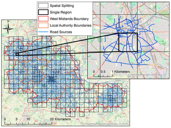
Figure 1.
Example of explicit road source truncation for a particular sub-region. A buffer zone of 750 m has been used. Note that spatial sub-regions outside the WM boundary are run in the model but not included in contour output, and thus are not shown here.
Conversely, point sources with high pollutant emission rates are always modelled explicitly due to their non-negligible buoyancy and elevated source height, which affect their dispersion over a long distance. Point sources are generally selected for explicit modelling if they have annual average emissions greater than 1 g/s of a pollutant of interest, or are subject to specific national regulation (“‘Part A” sources). The number of point sources of this type is often much smaller than the number of modelled road sources and so the run-time cost of including all point sources in each sub-region run, with extents normally of the order of 1 km, is comparatively small.
2.3. Case Study
The West Midlands Combined Authority (WMCA) in the UK covers seven constituent local authorities (Birmingham, Coventry, Dudley, Sandwell, Solihull, Walsall and Wolverhampton). Geographically, the West Midlands (WM) is an area of around 902 km2 roughly centred on Birmingham. Air quality modelling is an important tool for the investigation of air quality within the WM region and for the assessment of the impact of specific intervention scenarios on air quality within the region.
2.3.1. Emissions
Emission sources in the model included explicit point sources, explicit road sources and 1 km × 1 km horizontal resolution grid sources for the baseline year of 2016 (shown as Figure 2). The EMIT Atmospheric Emissions Inventory Toolkit (developed by CERC) was used to pre-process the emission data before import into the ADMS-Urban model. Table 1 shows an overview of total emissions for different source types over WM computational domain.
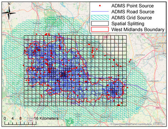
Figure 2.
Emission sources in the model and spatial splitting for the modelling domain over West Midlands.

Table 1.
Overview of total emissions (in tonnes/year) for different sources over the WM computational domain.
Point Sources
Point source emission rates were taken from the UK National Atmospheric Emissions Inventory (NAEI) [59], which collected detailed emission data from large individual sources. Other smaller emission sources in the industrial and commercial sector were included as grid sources (Section Grid Sources). Large industrial point sources were considered explicitly as elevated point sources in the dispersion model. The emission inventory for these point sources combined the NAEI 2016 data (for emission rates) and Birmingham City Council (BCC) Airviro [60] model data (for stack parameters, e.g., stack height and diameter, efflux temperature and exit velocity). Representative typical stack characteristics by sector were used for the point sources where the stack characteristics are not known. The emission rates from the point sources were given for a wide range of pollutants; those of interest are NOx as NO2, PM10, PM2.5, Non-Methane Volatile Organic Compounds (NMVOC) and SO2. The location of the point sources was given in the British National Grid Coordinate System (OSGB) and has been converted to the modelling coordinate system in Lambert Conformal Conic Projection (LCC). The use of modelling coordinate was consistent with that in the regional Community Multiscale Air Quality (CMAQ) modelling system, to prepare for the development of a coupling system between CMAQ and ADMS-Urban model under WM-Air.
Road Sources
Road sources in the current baseline model combined the traffic maps from Transport for West Midlands (TfWM) PRISM model [61] and BCC’s SATURN model [62]. The SATURN model has more road links within the forthcoming Clean Air Zone of Birmingham [63]. The traffic map covers major roads, e.g., motorways and “A” roads. Minor roads not represented by the current traffic map are modelled as grid sources. The traffic data for AM peak, PM peak and inter-peak time periods have been combined and converted into Annual Average Daily Traffic (AADT). The traffic flows were categorised into heavy and light vehicles. These traffic model output data were evaluated against the TfWM’s traffic count data. The light vehicle from the traffic model agrees well with traffic counts, while the heavy vehicle is consistently underestimated compared to traffic counts and an adjustment was made. Bus timetable data from Remix [64] were also processed and included in the model input. Representative fleet composition data (Euro classification for each sub-type of heavy and light vehicles) were taken from ANPR data in a recent Birmingham Clean Air Zone (CAZ) document [62] and has been incorporated into the EMIT calculations. The UK NAEI 2014 road traffic emission factors, with real-world adjustments following the approach described in Hood et al. 2018 [49], were used for the calculation of emission rates.
Grid Sources
Grid sources for 2016 were defined at 1 km × 1 km resolution with a typical depth of 10 m. The base gridded emissions were downloaded from the NAEI website [59] in the OSGB coordinate system, and have been converted to the LCC modelling coordinates. NAEI emissions are available for all SNAP (Selected Nomenclature for Air Pollution) sectors, i.e.,:
- SNAP 01—Combustion in Energy Production and Transformation (energyprod);
- SNAP02—Combustion in Commercial, Industrial, Residential and Agriculture (domcom);
- SNAP03—Combustion in Industry (indcom);
- SNAP04—Production Processes (indproc);
- SNAP05—Extraction and Distribution of Fossil Fuels (offshore);
- SNAP06—Solvent Use (solvents);
- SNAP07—Road Transport (roadtrans);
- SNAP08—Other Transport and Mobile Machinery (othertrans);
- SNAP09—Waste Treatment and Disposal (waste);
- SNAP10—Agriculture, Forestry and Landuse Change (agric);
- SNAP11—Nature (nature).
The pollutants of interest are NOx as NO2, NMVOC, PM10, PM2.5 and SO2. SNAP07 has been reduced by subtracting the emission contribution from the explicit major road sources. EMIT also aggregates the explicit major road emissions into the same 1 km × 1 km grid. The residual emission for this SNAP07 sector can be then derived and modelled as SNAP07_minor road.
2.3.2. Time Varying Factors
Time-varying factors from the EMEP model [65,66] were available for each hour of the day by SNAP sector and pollutant. An emissions inventory covering the area of interest was available, with total emission for each sector. These emission rates were used to calculate a combined set of weighted average monthly emission factors for each pollutant, which were applied to the total gridded emission rates. Separate time varying factors were applied to particulate and gaseous gridded emissions, reflecting different balances between sectors and source types for these pollutants. In additional to the gridded emission rates, time varying factors have been also applied to explicit road sources. The monthly factors used for explicit road source emissions were taken from Community Modelling and Analysis System (CAMS) regional emissions v3.1 [67]. Diurnal profiles for road traffic have been calculated using 24-h flow and speed data from automatic traffic count sites (data downloaded from TfWM), typically available for 1 week per site. The roads of interest were isolated, and the light and heavy vehicle hourly flows and speeds were processed through an Emissions Factor Toolkit (EFT, version 9.0) [68] spreadsheet to calculate hourly emission rates of the pollutant of interest. The emission rates were then normalised by the average emission rate on the road, to give a time varying profile for the road. The roads were classified into medium or high flow and average time-varying profiles were calculated for each type. The diurnal profile for medium roads was also applied to the grid source, representing both the significant contribution of minor roads to the residual gridded emissions and the representation of emissions from roads outside the current sub-region and buffer zones in the gridded emissions.
2.3.3. Background Data
Background concentration files were created using historic observation data from a variety of rural background sites surrounding the West Midlands modelling area, available from the Department for Environment, Food and Rural Affairs (Defra) UK-Air website [12]. Data were limited in the West Midlands area, so a suitable background file was created using the following sites for different pollutants: (1) NOx, NO2, O3: Ladybower (Lat, Lon: 53.403370, −0.752006), Market Harbough (52.554444, −0.772222), Chilbolton (51.149617, −1.438228), Leominster (52.221740, −2.736665), (2) SO2: Ladybower, Narberth (51.781784, −4.691462), Chilbolton and (3) PM10 and PM2.5: Chilbolton (with large periods of missing data filled using data from Sheffield Devonshire Green). The direction of each monitoring site from the centre of the modelling region, and wind direction sectors which were appropriate for each site, were calculated. The monitored wind direction for each hour was used to identify upwind monitoring data for that hour. The use of Chilbolton for particulate background concentrations was due to the fact that appropriate background monitoring sites for PM were scarce around the West Midlands area. The monitored Chilbolton concentration was multiplied by the ratio of the annual average concentration at a rural area bordering the West Midlands to that at Chilbolton based on Defra’s background concentration maps [69].
2.3.4. Meteorological Data
For the West Midlands, an appropriate synoptic meteorological measurement site is located at Birmingham Elmdon, within Birmingham Airport, with data obtained from Met Office MIDAS in CEDA Archive [70]. “UK Hourly weather data”, “UK Mean Wind” and “UK Hourly rainfall data” have been combined to create the met data format required by the model. The generated met file included hourly data for wind direction, wind speed (converted from knots to m/s), total cloud fraction, air temperature, relative humidity and precipitation.
2.3.5. Advanced Canyon and Urban Canopy Files
The data required to carry out the advanced canyon [51] and urban canopy [50] calculations are (1) a road network shapefile and (2) a buildings shapefile, including a height field. The building data have been obtained from Digimap database [71] via the University. The ADMS-Urban software package included ArcGIS tools [72] which have been used to calculate an Advanced Canyon file. The building height and canyon width along each road link were derived. The gridded urban canopy parameters have also been calculated for use in representing urban wind flow variations. These will enable the ADMS-Urban model to account for the street canyon effect for road emissions and spatially varying urban canopy flow for all source types.
2.3.6. Spatial Splitting
The task farming approach was achieved by spatially splitting the domain within the ADMS model. The overall rectangular output grid domain extent covering WM was first divided into 468 smaller sub-domains (forming a grid of 26 by 18 sub-domains, shown as Figure 2), each with a size of 2 km × 2 km. For some 2 km × 2 km subdomains with denser road links in city centre areas, which also included increased numbers of output points to fully resolve the near-road concentrations, a further spatial splitting into 1 km × 1 km or 500 m × 500 m was adopted in order to reduce the overall computation time. The total number of sub-domains was 540 (although no output points have been specified beyond 1 km outside the WM boundaries). The maximum number of road sources in a single sub-domain was 598 and the maximum number of output points in a domain was 4725. A buffer zone [73] of 750 m for road sources (to exclude explicit road sources unlikely to contribute significantly to modelled concentrations in the sub-domain) was used for each sub-domain.
3. Results
3.1. Receptor Run: Model Evaluation
For the purpose of model evaluation, the model was first run in a “Receptor” Mode (a run with output for a limited number of specified receptors) for 32 air quality measurement sites within the WM over the whole year of 2016, with measured concentration data obtained from local authorities and Defra’s AURN [12] (shown as Figure 3, mostly with available hourly air quality measurements). These sites included three types, i.e., 1 airport site, 19 roadside sites and 12 urban background sites. In order to reduce the model computational time, the source exclusion option [73] was used to not explicitly model road sources far away from specified receptors, and therefore unlikely to contribute significantly to modelled concentrations at receptors, with a specified exclusion distance of 750 m. The Receptor run was conducted in a Windows PC and it took about 12 h’ computation time to get the hourly output of five air pollutants (NOx, NO2, O3, PM10 and PM2.5) across a whole year for all 32 receptors. The Model Evaluation Toolkit [74] was used to conduct the evaluation of the model by comparing to the measured air quality data using statistical and graphical methods.
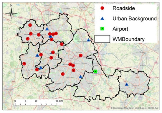
Figure 3.
Monitoring sites within West Midland used for the model evaluation.
3.1.1. NOx and Chemistry
Figure 4 shows the evaluation of modelled annual NOx, NO2 and O3 against observations using scatter plots divided by site type. Overall, the model performed well in terms of NOx and NO2 for all site types. The good fits for O3 further suggested good performance of the model chemistry. Table 2 shows the statistics (see definitions in [49]) for the model evaluation for the baseline year of 2016, calculated from the hourly modelled and measured concentrations. Fb (Fractional bias) measures the mean concentration difference between the model and measurement (ideal value is 0). Fac2 measures the fraction of modelled data within a factor of 2 of observations (ideal value is 1.0). NMSE (normalised mean square error) measures the mean concentration difference between matched pairs of modelled and measured data (ideal value is 0). R (correlation coefficient) measures a linear relationship of concentrations between the model and measurement (ideal value is 1.0). Fb varies between (−0.24, 0.03) for NOx and (−0.08, 0.06) for NO2 and O3, while (0, 0.05) for NOx and (−0.01, 0.06) for NO2 and O3 were derived for the ADMS-Urban run with adjusted road traffic in Hood et al. (2018) [49]. Fac2 indicates that more than 62% of NOx, 76% of NO2 and 73% of O3 are within a factor of 2 of observations. NMSE varies between (1.03, 1.24) for NOx, (0.12, 0.32) for NO2 and O3, which is similar to (0.62, 0.86) for NOx and (0.21, 0.29) for NO2 and O3 in Hood et al. (2018) [49]. R varies between (0.58, 0.83) for NOx, NO2 and O3, which is close to (0.61, 0.77) in Hood et al. (2018) [49].
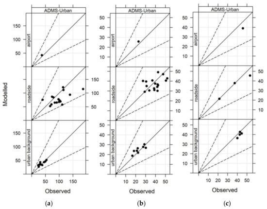
Figure 4.
Comparison of annual averages between model output and measurement: (a) for NOx (in μg m−3), (b) for NO2 (in μg m−3) and (c) for O3 (in μg m−3).
Table 2.
Statistics for model evaluation for the baseline year of 2016 calculated from the hourly modelled and measured concentrations. nSites: number of sites; Obs: observed concentration; Mod: modelled concentration; Fb: fraction bias (ideal value is 0); Fac2: fraction of modelled data within a factor of 2 of observations (ideal value is 1.0); NMSE: normalised mean square error (ideal value is 0); R: correlation coefficient (ideal value is 1.0).
3.1.2. PM10 and PM2.5
Figure 5 shows the evaluation of modelled annual average PM10 and PM2.5 against observations using scatter plots divided by site types; note that there were no PM2.5 measurements at the single airport site. PM10 had a very good fit for the airport and urban background sites. PM10 tended to slightly over-predict at roadside sites, possibly related to uncertainties in traffic non-exhaust emissions and background data. The model had good predictions for the small number of sites with available PM2.5 measurement data. For PM10 and PM2.5, Fb ranges between (−0.13, 0.12), slightly wider than (−0.07, 0.09) in Hood et al. (2018) [49]. Fac2 indicates that more than 74% of PM10 and PM2.5 are within a factor of 2 of observations. NMSE varies between (0.43, 0.53) for PM10 and PM2.5, slightly higher than (0.27, 0.37) in Hood et al. (2018) [49]. R varies between (0.48, 0.66) for PM10 and PM2.5, slightly lower than (0.58, 0.77) in Hood et al. (2018) [49].
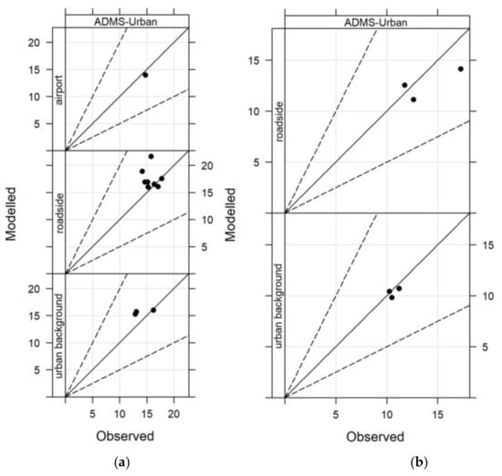
Figure 5.
Comparison of annual averages between model output and measurement: (a) for PM10 (in μg m−3); (b) for PM2.5 (in μg m−3).
3.2. Contour Run: Air Quality Maps
For the generation of air quality maps, the model was then run in a “Contour” Mode (with the splitting option activated) to include output points covering the whole WM (and extending up to 1 km outside the WM boundary). An array job with 540 cores, each for a single sub-domain as shown in Figure 2, was submitted to the HPC at the University of Birmingham using the Linux version of the ADMS-Urban model. The overall elapsed time for the run (determined by the slowest core of 540 cores) for the typical whole year 2016 baseline case is about 35 h, with a median core run time of about 5 h and a minimum run time of 16 s for sub-domains without any emission sources. The total computational time (summing over all 540 cores) is about 169 days. Figure 6 shows a comparison of elapsed (clock) time of the slowest core and total computational time using task farming, (estimated by a typical one day simulation due to the substantial computational time requirement for a single core simulation). From 1 core to 4 core, the typical elapsed time can reduce by about 80%. From 156 cores, the typical elapsed time reduces more gradually. The total computational time profile has a slower decrease than the profile for the elapsed time of the slowest core, which is due to the increase in the buffer zone calculations for larger numbers of cores (especially for 540 cores). The choice of the number of cores can be dependent on the local HPC service, such as limitations in the number of available cores and the maximum allowed time for a single core (walltime).
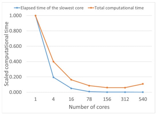
Figure 6.
Comparison of elapsed (clock) time of the slowest core and total computational time using task farming; note that the horizontal axis scale is non-linear.
The output for each subdomain was in netcdf file format, which has been combined and interpolated using the CombineCOF and AddInterpIGP utilities developed by CERC. The re-combination and interpolation time was about 1 h. The recombined and interpolated outputs for the hourly output of the whole year over WM region contained ~0.61 million and ~1.26 million output locations, and had file sizes of about 120 GB and 247 GB, respectively. The final netcdf output was then processed to derive annual/subset averages and other statistical output (e.g., percentiles) using the “Process comprehensive output” tool in the model. This process took a couple of hours, dependent on the number of output air pollutants. The final contour plots over WM at a specified resolution (e.g., 10 m × 10 m) were created via GIS tools, in particular using interpolation in Surfer and display in ArcGIS.
3.2.1. Annual Air Quality Map
Figure 7 presents a map of the annual average NO2 concentration which is a key air quality challenge for roadside locations in the UK, at 10 m × 10 m horizontal resolution for the baseline year of 2016. Other pollutants such as NOx, O3, PM10 and PM2.5 are shown in Figure A1. The legend of Figure 7 indicates colour scales with annual mean NO2 concentrations higher than the UK objective value of 40 μg m−3 [75] shown in orange and red. There were relatively higher concentrations of NO2 near motorways and major roads in city centre areas, mostly due to the higher traffic-related emissions. Away from major roads and in rural areas, NO2 concentrations were generally lower.
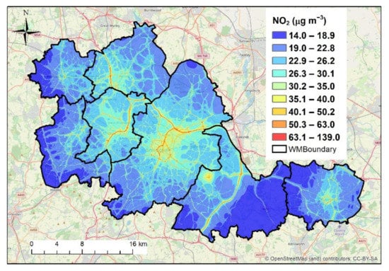
Figure 7.
Annual air quality maps for NO2 (in μg m−3) at 10 m × 10 m resolution. Areas exceeding the UK objective value of 40 μg m−3 are shown in yellow, orange and red.
3.2.2. Projected Air Quality Map for Health
For the purposes of health-related research, including assessment of personal exposure and exploration of relationships between air pollution levels and socio-demographic characteristics typically available on different spatial scales, the 10 m × 10 m horizontal resolution annual air quality map may need to be further aggregated into other polygon layers, e.g., Lower Layer Super Output Areas (LSOA) and ward levels (averages over these layers). Figure 8 shows examples of projected annual air quality maps for NO2 averaged over LSOA layer and ward level layer. There were clear patterns of higher concentration in city centre areas and lower concentration in rural areas. The projected air quality maps for other pollutants such as NOx, O3, PM10 and PM2.5 are shown in Figure A2 (in LSOA layer) and Figure A3 (in the ward layer). These can then be linked to population and health data for the assessment of the health impacts of air pollution. Note that the spatial averaging process leads to a narrower range of concentrations across the whole area, as both the lowest concentrations in the most rural areas and the highest concentrations adjacent to road sources are no longer fully represented; this reduction in dynamic range is significant and dependent on spatial resolution.
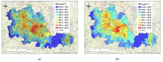
Figure 8.
Projected annual air quality maps for NO2 (in μg m−3) (a) in the Lower Layer Super Output Areas (LSOA) layer and (b) in the ward level.
3.2.3. Percentile Air Quality Map
Apart from annual average air quality targets, percentiles are also a useful indicator for the exceedance of the air quality objective value. For NO2, the 99.8 percentile for the 1 h mean [75] is normally used, which represents the 18th highest concentration in hourly series over a whole calendar year. The UK objective for 1 h mean NO2 concentration (where public exposure occurs) is “200 μg m−3 not to be exceeded more than 18 times a year” [75]. Figure 9 shows the 99.8 percentile for 1 h mean NO2 concentration. The exceedance of air quality objective value (200 μg m−3) for 1 h NO2 concentration was found mostly along motorways and major roads linking to motorways, areas in which public exposure may be limited.
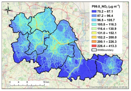
Figure 9.
The 99.8 percentile annual air quality maps for 1 h mean NO2 (in μg m−3) at 10 m × 10 m resolution. Areas exceeding the UK objective value of 200 μg m−3 are shown in orange and red.
3.2.4. Air Quality Maps over Temporal Subsets
Post-processing tools provide the flexibility to obtain concentration averages over temporal subsets, which may be useful when mapped for health/exposure study. Figure 10 shows air quality maps of NO2 over selected temporal subsets, i.e., AM (7 a.m.–9 a.m.) weekday, IP (inter-Peak) (9 a.m.–3 p.m.) weekday, PM (3 p.m.–7 p.m.) weekday, and IP (9 a.m.–3 p.m.) weekend. For AM weekday and PM weekday, the influence of major road emissions is clearly visible over the whole WM region, due to the region-wide increased traffic activity during these peak periods. For IP weekday and IP weekend, the major roads have a lesser contribution to concentrations over the WM region, compared with peak periods on weekdays. The NO2 concentration for IP weekday shows higher overall concentration levels and a clearer pattern of influence from road emissions than that for IP weekend.
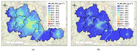
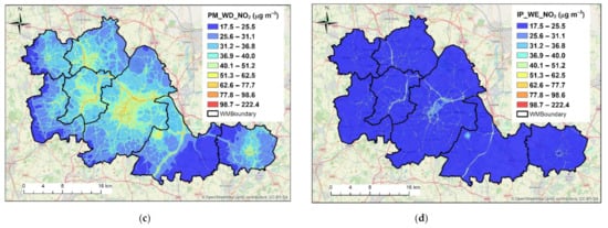
Figure 10.
Air quality maps for NO2 (in μg m−3) at 10 m × 10 m resolution averaged over (a) AM weekday, (b) IP weekday, (c) PM weekday, (d) IP weekend.
4. Discussion
The air quality sites used to evaluate the model performance included three representative types (i.e., airport, roadside and urban background sites). Overall, the model performed well for all pollutants. For airport and urban background sites, the model results reproduce the measured values well since these are less influenced by local emissions and complex building geometry. For roadside sites, the concentrations of air pollutants are more influenced by local emission (e.g., traffic NOx) and street canyon geometry, which may be reflected in higher uncertainty for some of the roadside sites. NOx and NO2 concentration levels are most closely related to local emissions and can be well predicted by the current model. PM concentrations are more related to the regional background, which may have some uncertainty. In order to reduce the model uncertainty, the model has been set up with the best available emissions, meteorology, building data, source locations and monitor locations for the WM region. From the model best practice and model evaluation, the model configuration is satisfactory for the wider WM contour run. It is of note that, for PM10 and PM2.5, the background concentrations (constrained to observations) are greater than the increment associated with emissions in the model domain at all sites.
The contour run was performed by using the modelling capability of task farming (via spatial splitting) within the ADMS-Urban model. For this air quality modelling application in a large urban area, the optimisation process has reduced weeks of model execution time to only ~35 h and the model can generate high horizontal resolution “street-scale” air quality maps over WM. There are relatively higher annual concentrations of NO2 in city centre areas (e.g., Birmingham), mainly due to the higher local traffic emissions. As NO2 concentrations are closely related to local traffic emissions, the control of traffic in city centre areas would have a substantial effect on reducing proximate NO2 levels. A Birmingham CAZ is proposed to be in place from June 2021 to reduce air pollution levels within Birmingham city centre [63].
The high horizontal resolution air quality maps generated from the model output can be further aggregated into other health-related layers (such as LSOA and ward layers) to study the relationship between air quality and health data. Apart from the annual averages, the model output and post-processing flexibility enables the calculation of other statistics, such as percentiles. Exceedances of the air quality objective value for the 99.8 percentile of the 1 h mean NO2 concentration were generally only found for motorways and major roads directing to motorways, which is unsurprising due to intensive traffic activity. The reduction in traffic speed limits for some motorways (e.g., trials on speed limits on M6 and M5 motorways near Birmingham reduced from 70 mph to 60 mph by Highways England [76]) may thus help to reduce the NO2 exceedance, although exposure at such locations may be limited.
Air quality maps over temporal subsets can be also derived for health/exposure study. As expected, AM weekday and PM weekday have clear patterns of region-wide traffic, while NO2 concentrations over these periods are much higher than the annual averages. The influences of traffic over IP weekday and IP weekend are less significant compared with AM weekday and PM weekday. These findings can be useful for exposure and health studies over working periods. Reis et al. [77] also highlighted the importance of workday population mobility on the exposure to air pollutants.
5. Conclusions
A WM-Air ADMS-Urban baseline model configuration has been developed and model predictions for NOx, NO2, O3, PM10 and PM2.5 have been evaluated using measurement data. Overall, the model performed well and run times are manageable using the task farming approach. A regional (e.g., CMAQ) modelling system can provide spatially varying regional background predictions, which can be coupled with the ADMS-Urban model in future, but may also have its own uncertainties in terms of model configuration, compared with observational constraints. The post-processing flexibility enables the creation of air quality maps for annual/subset averages and other statistical output (e.g., percentiles). The model outputs can be useful for the study of health impacts of air pollutants.
Future work will draw upon the demonstrated efficient execution of multiple air quality modelling scenarios on HPC. It is important to ensure that the model configuration includes model inputs that are sufficiently detailed that they allow different scenarios to be represented. There are a range of possible air quality modelling scenarios: local and national, short-term and long-term, transport related and non-transport related. The combination of detailed inventory and spatially defined emissions, high resolution dispersion simulation, efficient parallelisation and flexible post-processing will allow the exploration of multiple scenarios. These may investigate concentration responses to interventions such as Clean Air Zones, the influence of solid fuel combustion, agricultural emissions, air quality–climate interactions and the relationships between air pollution exposure and population distribution. These in turn enable optimisation of combined benefits and equity of possible future limit value and exposure reduction based on air quality targets.
Author Contributions
Conceptualisation, X.C.; methodology, C.H. and K.J.; software, J.S. and J.H.; validation, K.J. and C.H.; formal analysis, J.Z.; investigation, J.Z.; resources, X.C., M.W. and A.M.; data curation, K.J., C.H. and J.Z.; writing—original draft preparation, J.Z. and C.H.; writing—review and editing, A.M., J.S. and W.J.B.; visualisation, J.Z.; supervision, J.S., J.H., M.W. and X.C.; project administration, J.S. and X.C.; funding acquisition, W.J.B. All authors have read and agreed to the published version of the manuscript.
Funding
This research was funded by the UK Natural Environment Research Council (NERC) project WM-Air, grant number NE/S003487/1.
Institutional Review Board Statement
Not applicable.
Data Availability Statement
AURN data are available via Defra website, https://uk-air.defra.gov.uk/networks/network-info?view=aurn (accessed on 18 June 2019). The NAEI emission data are available via http://naei.beis.gov.uk/data (accessed on 18 July 2019). The traffic data may be accessed subject to a license with TfWM/BCC. MIDAS met data are available via http://data.ceda.ac.uk/badc (accessed on 14 January 2019). EMEP time-variation data are available via https://www.emep.int/. The building data are available via https://digimap.edina.ac.uk (accessed on 28 May 2019). Other data (e.g., modelling output) may be made available upon request.
Acknowledgments
The authors appreciate the University of Birmingham’s BlueBEAR HPC service (http://www.bear.bham.ac.uk, accessed on 23 April 2021) for providing the computational resource. The authors would like to acknowledge local authorities within WM for provision of local air quality measurement and modelling data and for their review of local emissions data, with special thanks to John Grant and Curtis Dean in Walsall council. The authors also thank Transport for West Midlands (TfWM) and Birmingham City Council for provision of traffic data, previous modelling and reports.
Conflicts of Interest
The authors declare no conflict of interest.
Appendix A
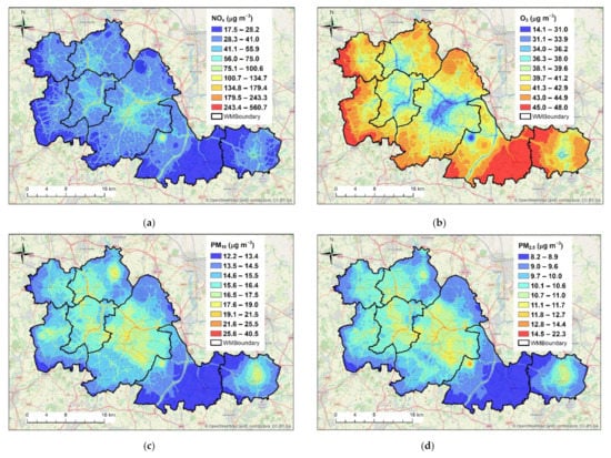
Figure A1.
Annual air quality maps for (a) NOx (in μg m−3), (b) O3 (in μg m−3), (c) PM10 (in μg m−3) and (d) PM2.5 (in μg m−3) at 10 m × 10 m resolution.
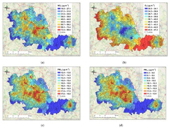
Figure A2.
Projected annual air quality maps for (a) NOx (in μg m−3), (b) O3 (in μg m−3), (c) PM10 (in μg m−3) and (d) PM2.5 (in μg m−3) in the Lower Layer Super Output Areas (LSOA) layer.
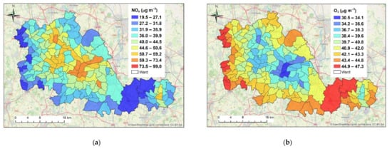

Figure A3.
Projected annual air quality maps for (a) NOx (in μg m−3), (b) O3 (in μg m−3), (c) PM10 (in μg m−3) and (d) PM2.5 (in μg m−3) in the ward level.
References
- WHO. Available online: https://www.who.int/news-room/fact-sheets/detail/ambient-(outdoor)-air-quality-and-health (accessed on 11 January 2021).
- Xu, J.; Srivastava, D.; Wu, X.; Hou, S.; Vu, T.V.; Liu, D.; Sun, Y.; Vlachou, A.; Moschos, V.; Salazar, V.; et al. An evaluation of source apportionment of fine OC and PM 2.5 by multiple methods: APHH-Beijing campaigns as a case study. Faraday Discuss. 2020, 226, 290–313. [Google Scholar] [CrossRef]
- Gordon, T.; Balakrishnan, K.; Dey, S.; Rajagopalan, S.; Thornburg, J.; Thurston, G.; Agrawal, A.; Collman, G.; Guleria, R.; Limaye, S.; et al. Air pollution health research priorities for India: Perspectives of the Indo-US Communities of Researchers. Environ. Int. 2018, 119, 100–108. [Google Scholar] [CrossRef]
- UK_gov. Available online: https://assets.publishing.service.gov.uk/government/uploads/system/uploads/attachment_data/file/633270/air-quality-plan-detail.pdf (accessed on 11 January 2021).
- Hu, F.P.; Guo, Y.M. Health impacts of air pollution in China. Front. Environ. Sci. Eng. 2021, 15, 1–18. [Google Scholar] [CrossRef]
- WHO. Available online: https://www.who.int/phe/publications/air-pollution-global-assessment/en/ (accessed on 11 January 2021).
- Shaddick, G.; Thomas, M.L.; Mudu, P.; Ruggeri, G.; Gumy, S. Half the world’s population are exposed to increasing air pollution. Npj Clim. Atmos. Sci. 2020, 3, 1–5. [Google Scholar] [CrossRef]
- WHO. Available online: https://www.who.int/teams/environment-climate-change-and-health/air-quality-and-health/ambient-air-pollution (accessed on 11 January 2021).
- COMEAP. Available online: https://www.gov.uk/government/publications/nitrogen-dioxide-effects-on-mortality/associations-of-long-term-average-concentrations-of-nitrogen-dioxide-with-mortality-2018-comeap-summary (accessed on 24 May 2021).
- McLaren, J.; Williams, I.D. The impact of communicating information about air pollution events on public health. Sci. Total Environ. 2015, 538, 478–491. [Google Scholar] [CrossRef] [PubMed]
- Delmas, M.A.; Kohli, A. Can Apps Make Air Pollution Visible? Learning About Health Impacts Through Engagement with Air Quality Information. J. Bus. Ethics 2020, 161, 279–302. [Google Scholar] [CrossRef] [Green Version]
- Defra. Available online: https://uk-air.defra.gov.uk/networks/network-info?view=aurn (accessed on 18 June 2019).
- Wesseling, J.; de Ruiter, H.; Blokhuis, C.; Drukker, D.; Weijers, E.; Volten, H.; Vonk, J.; Gast, L.; Voogt, M.; Zandveld, P.; et al. Development and Implementation of a Platform for Public Information on Air Quality, Sensor Measurements, and Citizen Science. Atmosphere 2019, 10, 445. [Google Scholar] [CrossRef] [Green Version]
- Samad, A.; Vogt, U. Mobile air quality measurements using bicycle to obtain spatial distribution and high temporal resolution in and around the city center of Stuttgart. Atmos. Environ. 2021, 244, 117915. [Google Scholar] [CrossRef]
- Elen, B.; Peters, J.; Van Poppel, M.; Bleux, N.; Theunis, J.; Reggente, M.; Standaert, A. The Aeroflex: A Bicycle for Mobile Air Quality Measurements. Sensors 2013, 13, 221–240. [Google Scholar] [CrossRef]
- Hagemann, R.; Corsmeier, U.; Kottmeier, C.; Rinke, R.; Wieser, A.; Vogel, B. Spatial variability of particle number concentrations and NOx in the Karlsruhe (Germany) area obtained with the. mobile laboratory ‘AERO-TRAM’. Atmos. Environ. 2014, 94, 341–352. [Google Scholar] [CrossRef] [Green Version]
- de Vries, J.; Loenen, E.; Mijling, B.; van der Meulen, W.; van der Meer, A. Satellite and Local Measurements Based Services for Air Quality Improvement. Asian J. Atmos. Environ. 2019, 13, 39–44. [Google Scholar] [CrossRef]
- EEA. Available online: https://www.eea.europa.eu/publications/fairmode (accessed on 25 February 2021).
- EUR-Lex. Available online: https://eur-lex.europa.eu/legal-content/EN/TXT/?uri=celex%3A32008L0050 (accessed on 25 February 2021).
- AIR-EIA. Available online: http://www.ess.co.at/AIR-EIA/LECTURES/L001.html (accessed on 25 February 2021).
- Lamb, R.G.; Seinfeld, J.H. Mathematical modeling of urban air pollution. General theory. Environ. Sci. Technol. 1973, 7, 253–261. [Google Scholar] [CrossRef] [PubMed]
- Pasquill, F. The Estimation of The Dispersion of Windborne Material. Meteorol. Mag. 1961, 90, 33–40. [Google Scholar]
- Pasquill, F. Some observed properties of medium-scale diffusion in the atmosphere. Q. J. R. Meteorol. Soc. 1962, 88, 70–79. [Google Scholar] [CrossRef]
- SCOPE. Available online: https://storage.googleapis.com/carnegie-dge-scope-mirror/SCOPE_30/SCOPE_30_2.28_Piver_635-650.pdf (accessed on 25 February 2021).
- Liu, M.-K.; Seinfeld, J.H. On the validity of grid and trajectory models of urban air pollution. Atmos. Environ. 1975, 9, 555–574. [Google Scholar] [CrossRef]
- Friedlander, S.K.; Seinfeld, J.H. Dynamic model of photochemical smog. Environ. Sci. Technol. 1969, 3, 1175–1181. [Google Scholar] [CrossRef]
- Fisher, B.E.A. The long range transport of sulphur dioxide. Atmos. Environ. 1975, 9, 1063–1070. [Google Scholar] [CrossRef]
- El-Harbawi, M. Air quality modelling, simulation, and computational methods: A review. Environ. Rev. 2013, 21, 149–179. [Google Scholar] [CrossRef]
- Russo, A.; Raischel, F.; Lind, P.G. Air quality prediction using optimal neural networks with stochastic variables. Atmos. Environ. 2013, 79, 822–830. [Google Scholar] [CrossRef] [Green Version]
- Voukantsis, D.; Karatzas, K.; Kukkonen, J.; Räsänen, T.; Karppinen, A.; Kolehmainen, M. Intercomparison of air quality data using principal component analysis, and forecasting of PM₁₀ and PM₂.₅ concentrations using artificial neural networks, in Thessaloniki and Helsinki. Sci. Total Environ. 2011, 409, 1266–1276. [Google Scholar] [CrossRef]
- Gardner, M.W.; Dorling, S.R. Artificial neural networks (the multilayer perceptron)—A review of applications in the atmospheric sciences. Atmos. Environ. 1998, 32, 2627–2636. [Google Scholar] [CrossRef]
- Thunis, P.; Miranda, A.; Baldasano, J.M.; Blond, N.; Douros, J.; Graff, A.; Janssen, S.; Juda-Rezler, K.; Karvosenoja, N.; Maffeis, G.; et al. Overview of current regional and local scale air quality modelling practices: Assessment and planning tools in the EU. Environ. Sci. Policy 2016, 65, 13–21. [Google Scholar] [CrossRef]
- Carnevale, C.; Finzi, G.; Guariso, G.; Pisoni, E.; Volta, M. Surrogate models to compute optimal air quality planning policies at a regional scale. Environ. Modell. Softw. 2012, 34, 44–50. [Google Scholar] [CrossRef]
- Skamarock, W.C.; Klemp, J.B. A time-split nonhydrostatic atmospheric model for weather research and forecasting applications. J. Comput. Phys. 2008, 227, 3465–3485. [Google Scholar] [CrossRef]
- Chemel, C.; Fisher, B.E.A.; Kong, X.; Francis, X.V.; Sokhi, R.S.; Good, N.; Collins, W.J.; Folberth, G.A. Application of chemical transport model CMAQ to policy decisions regarding PM2.5 in the UK. Atmos. Environ. 2014, 82, 410–417. [Google Scholar] [CrossRef] [Green Version]
- Grell, G.A.; Peckham, S.E.; Schmitz, R.; McKeen, S.A.; Frost, G.; Skamarock, W.C.; Eder, B. Fully coupled "online" chemistry within the WRF model. Atmos. Environ. 2005, 39, 6957–6975. [Google Scholar] [CrossRef]
- Hu, J.L.; Li, X.; Huang, L.; Ying, Q.; Zhang, Q.; Zhao, B.; Wang, S.X.; Zhang, H.L. Ensemble prediction of air quality using the WRF/CMAQ model system for health effect studies in China. Atmos. Chem. Phys. 2017, 17, 13103–13118. [Google Scholar] [CrossRef] [Green Version]
- San Jose, R.; Perez, J.L.; Perez, L.; Barras, R.M.G. Effects of climate change on the health of citizens modelling urban weather and air pollution. Energy 2018, 165, 53–62. [Google Scholar] [CrossRef]
- Liu, H.; Deng, Y.; Lu, C.; Zhang, X.; Yang, X.; Song, D.; Tan, Q. A CMAQ-based Study on Evaluation of Achievements of Measures on Ozone Pollution Prevention and Control in Summer 2017 in Chengdu. IOP Conf. Ser. Earth Environ. Sci. 2020, 610, 012015. [Google Scholar] [CrossRef]
- Cheng, F.Y.; Feng, C.Y.; Yang, Z.M.; Hsu, C.H.; Chan, K.W.; Lee, C.Y.; Chang, S.C. Evaluation of real-time PM2.5 forecasts with the WRF-CMAQ modeling system and weather-pattern-dependent bias-adjusted PM2.5 forecasts in Taiwan. Atmos. Environ. 2021, 244, 117909. [Google Scholar] [CrossRef]
- Zlatev, Z.; Brandt, J.; Builtjes, P.J.H.; Carmichael, G.; Dimov, I.; Dongarra, J.; Dop, H.V.; Georgiev, K.; Hass, H.; José, R.S. Large Scale Computations in Air Pollution Modelling, 1st ed.; Springer: Dordrecht, The Netherlands, 1999; pp. 1173–1184. [Google Scholar]
- Dabdub, D.; Seinfeld, J.H. Air quality modeling on massively parallel computers. Atmos. Environ. 1994, 28, 1679–1687. [Google Scholar] [CrossRef]
- Dagum, L.; Menon, R. OpenMP: An industry standard API for shared-memory programming. IEEE Comput. Sci. Eng. 1998, 5, 46–55. [Google Scholar] [CrossRef] [Green Version]
- Sunderam, V.S. PVM: A framework for parallel distributed computing. Concurr. Pract. Exper. 1990, 2, 315–339. [Google Scholar] [CrossRef]
- Aoyama, Y.; Nakano, J. RS/6000 SP: Practical MPI Programming; International Technical Support Organisation, IBM Corporation: Austin, TX, USA, 1999; pp. 11–37. [Google Scholar]
- Kolodziej, J.; Pop, F.; Dobre, C. Modeling and Simulation in HPC and Cloud Systems; Springer International Publishing: Cham, Switzerland, 2018; pp. 45–57. [Google Scholar]
- Delic, G. Exploring parallel processing opportunities in AERMOD. In Proceedings of the 15th Annual CMAS Conference, Chapel Hill, NC, USA, 24–26 October 2016. [Google Scholar]
- Owen, B.; Edmunds, H.A.; Carruthers, D.J.; Singles, R.J. Prediction of total oxides of nitrogen and nitrogen dioxide concentrations in a large urban area using a new generation urban scale dispersion model with integral chemistry model. Atmos. Environ. 2000, 34, 397–406. [Google Scholar] [CrossRef]
- Hood, C.; MacKenzie, I.; Stocker, J.; Johnson, K.; Carruthers, D.; Vieno, M.; Doherty, R. Air quality simulations for London using a coupled regional-to-local modelling system. Atmos. Chem. Phys. 2018, 18, 11221–11245. [Google Scholar] [CrossRef] [Green Version]
- Hood, C.; Carruthers, D.; Seaton, M.; Stocker, J.; Johnson, K. Urban canopy flow field and advanced street canyon modelling in ADMS-Urban. In Proceedings of the 16th International Conference on Harmonisation, Varna, Bulgaria, 8–11 September 2014; pp. 8–11. [Google Scholar]
- Hood, C.; Stocker, J.; Seaton, M.; Johnson, K.; O’Neill, J.; Thorne, L.; Carruthers, D. Comprehensive evaluation of an advanced street canyon air pollution model. J. Air Waste Manag. Assoc. 2021, 71, 247–267. [Google Scholar] [CrossRef] [PubMed]
- Biggart, M.; Stocker, J.; Doherty, R.M.; Wild, O.; Hollaway, M.; Carruthers, D.; Li, J.; Zhang, Q.; Wu, R.L.; Kotthaus, S.; et al. Street-scale air quality modelling for Beijing during a winter 2016 measurement campaign. Atmos. Chem. Phys. 2020, 20, 2755–2780. [Google Scholar] [CrossRef] [Green Version]
- WM-Air. Available online: https://wm-air.org.uk/ (accessed on 10 May 2021).
- CERC. Available online: http://www.cerc.co.uk/environmental-software/assets/data/doc_techspec/P10_01.P12_01.pdf (accessed on 26 March 2021).
- CERC. Available online: http://www.cerc.co.uk/environmental-software/assets/data/doc_techspec/P31_01.pdf (accessed on 26 March 2021).
- CERC. Available online: http://www.cerc.co.uk/environmental-software/assets/data/doc_techspec/P18_03.pdf (accessed on 26 March 2021).
- Venkatram, A.; Karamchandani, P.; Pai, P.; Goldstein, R. The development and application of a simplified ozone modeling system (SOMS). Atmos. Environ. 1994, 28, 3665–3678. [Google Scholar] [CrossRef]
- Stocker, J.; Ellis, A.; Smith, S.; Carruthers, D.; Venkatram, A.; Dale, W.; Attree, M. A review of dispersion modelling of agricultural emissions with non-point sources. Int. J. Environ. Pollut. 2017, 62, 247–263. [Google Scholar] [CrossRef]
- NAEI. 2019. Available online: http://naei.beis.gov.uk/data (accessed on 18 July 2019).
- Airviro. Available online: http://80.229.174.184/iairviro/ (accessed on 31 October 2018).
- PRISM. 2019. Available online: https://www.tfwm.org.uk/strategy/data-insight/transport-modelling/about-prism (accessed on 22 July 2019).
- BCC_Report. 2018. Available online: https://www.birmingham.gov.uk/download/downloads/id/11353/aq3_-_birmingham_caz_fbc_report-_air_quality_v3_4-12-18.pdf+&cd=1&hl=zh-CN&ct=clnk&gl=uk (accessed on 1 October 2019).
- BCC. Available online: https://www.birmingham.gov.uk/info/20076/pollution/1763/a_clean_air_zone_for_birmingham (accessed on 2 May 2021).
- Remix. Available online: platform.remix.com (accessed on 9 April 2019).
- Simpson, D.; Benedictow, A.; Berge, H.; Bergström, R.; Emberson, L.D.; Fagerli, H.; Flechard, C.R.; Hayman, G.D.; Gauss, M.; Jonson, J.E.; et al. The EMEP MSC-W chemical transport model—Technical description. Atmos. Chem. Phys. 2012, 12, 7825–7865. [Google Scholar] [CrossRef] [Green Version]
- EMEP. Available online: https://www.emep.int/ (accessed on 17 May 2021).
- ECCAD. Available online: https://eccad.aeris-data.fr/ (accessed on 19 May 2021).
- EFT. Available online: https://laqm.defra.gov.uk/review-and-assessment/tools/emissions-factors-toolkit.html (accessed on 12 August 2019).
- Defra. Available online: https://uk-air.defra.gov.uk/data/laqm-background-home (accessed on 18 June 2019).
- CEDA. Available online: http://data.ceda.ac.uk/badc (accessed on 14 January 2019).
- Digimap. Available online: https://digimap.edina.ac.uk (accessed on 28 May 2019).
- Jackson, M.; Hood, C.; Johnson, C.; Johnson, K. Calculation of Urban Morphology Parameterisations for London for use with the ADMS-Urban Dispersion Model. Int. J. Adv. Remote Sens. GIS 2016, 5, 1678–1687. [Google Scholar] [CrossRef] [Green Version]
- CERC. ADMS-Urban User Guide Version 5.0. Available online: https://www.cerc.co.uk/environmental-software/assets/data/doc_userguides/CERC_ADMS-Urban5.0_User_Guide.pdf (accessed on 26 March 2021).
- Stidworthy, A.; Jackson, M.; Johnson, K.; Carruthers, D.; Stocker, J. Evaluation of local and regional air quality forecasts for London. Int. J. Environ. Pollut. 2018, 64, 178–191. [Google Scholar] [CrossRef]
- Defra. Available online: https://uk-air.defra.gov.uk/assets/documents/Air_Quality_Objectives_Update.pdf (accessed on 10 May 2021).
- HIghwaysEngland. Available online: https://highwaysengland.co.uk/our-work/air-quality/air-quality-speed-limit-trials/ (accessed on 10 May 2021).
- Reis, S.; Liška, T.; Vieno, M.; Carnell, E.J.; Beck, R.; Clemens, T.; Dragosits, U.; Tomlinson, S.J.; Leaver, D.; Heal, M.R. The influence of residential and workday population mobility on exposure to air pollution in the UK. Environ. Int. 2018, 121, 803–813. [Google Scholar] [CrossRef] [PubMed]
Publisher’s Note: MDPI stays neutral with regard to jurisdictional claims in published maps and institutional affiliations. |
© 2021 by the authors. Licensee MDPI, Basel, Switzerland. This article is an open access article distributed under the terms and conditions of the Creative Commons Attribution (CC BY) license (https://creativecommons.org/licenses/by/4.0/).