
A Study of Traffic Emissions Based on Floating Car Data for Urban Scale Air Quality Applications

 ,
, 
 ,
,  , ,
, , 
Abstract
:1. Introduction
2. Methodology
2.1. Road Traffic SMTS Data
2.2. Emission Processors
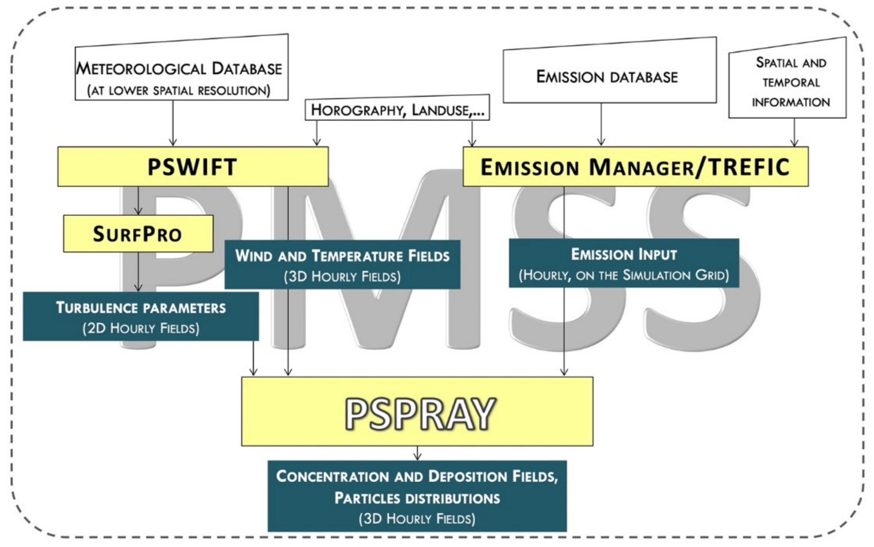
2.3. Dispersion Model
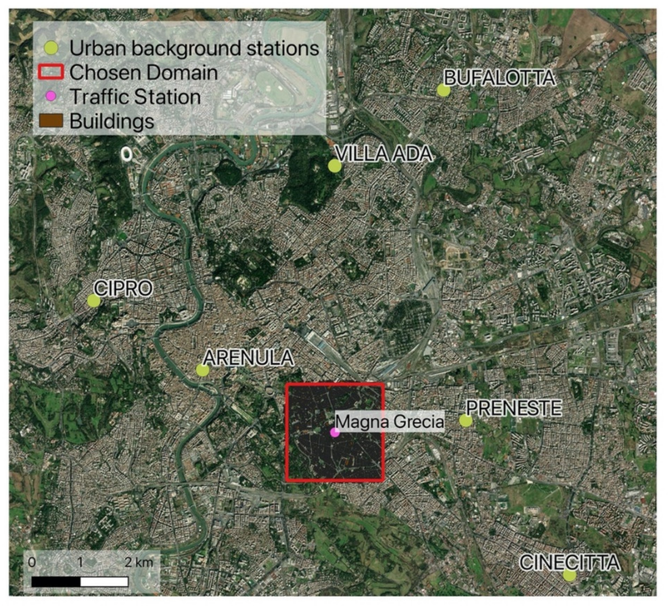
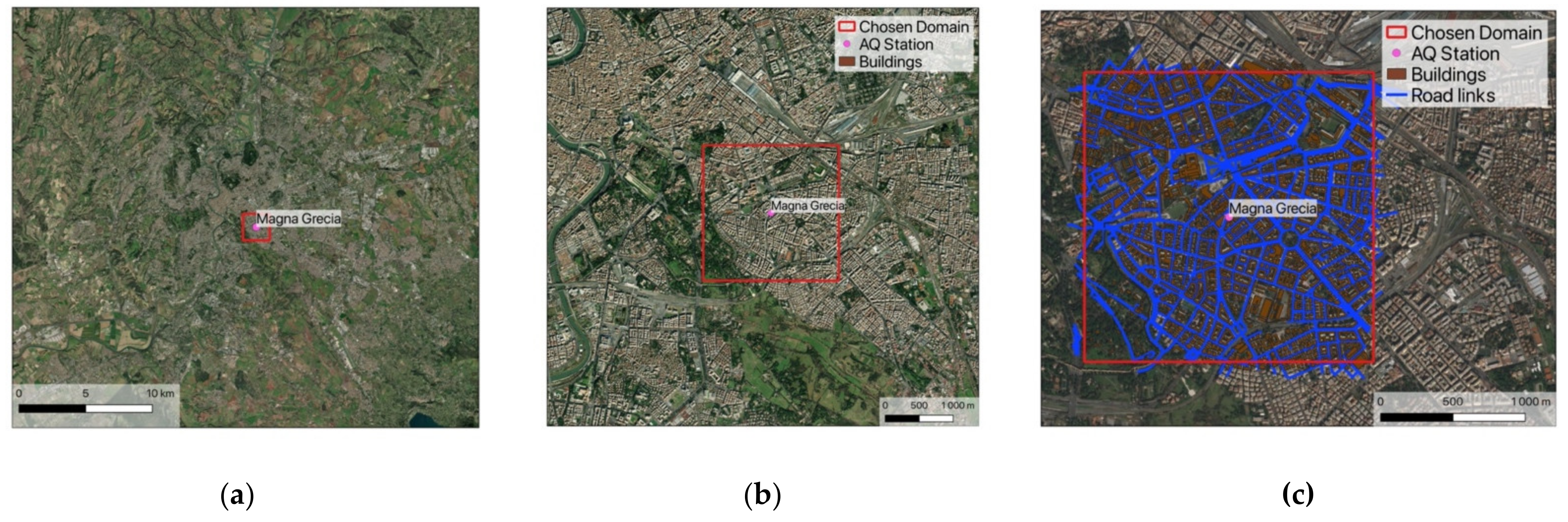
2.4. Simulation Setup
2.4.1. Input Meteorological Data
2.4.2. Emissions
- -
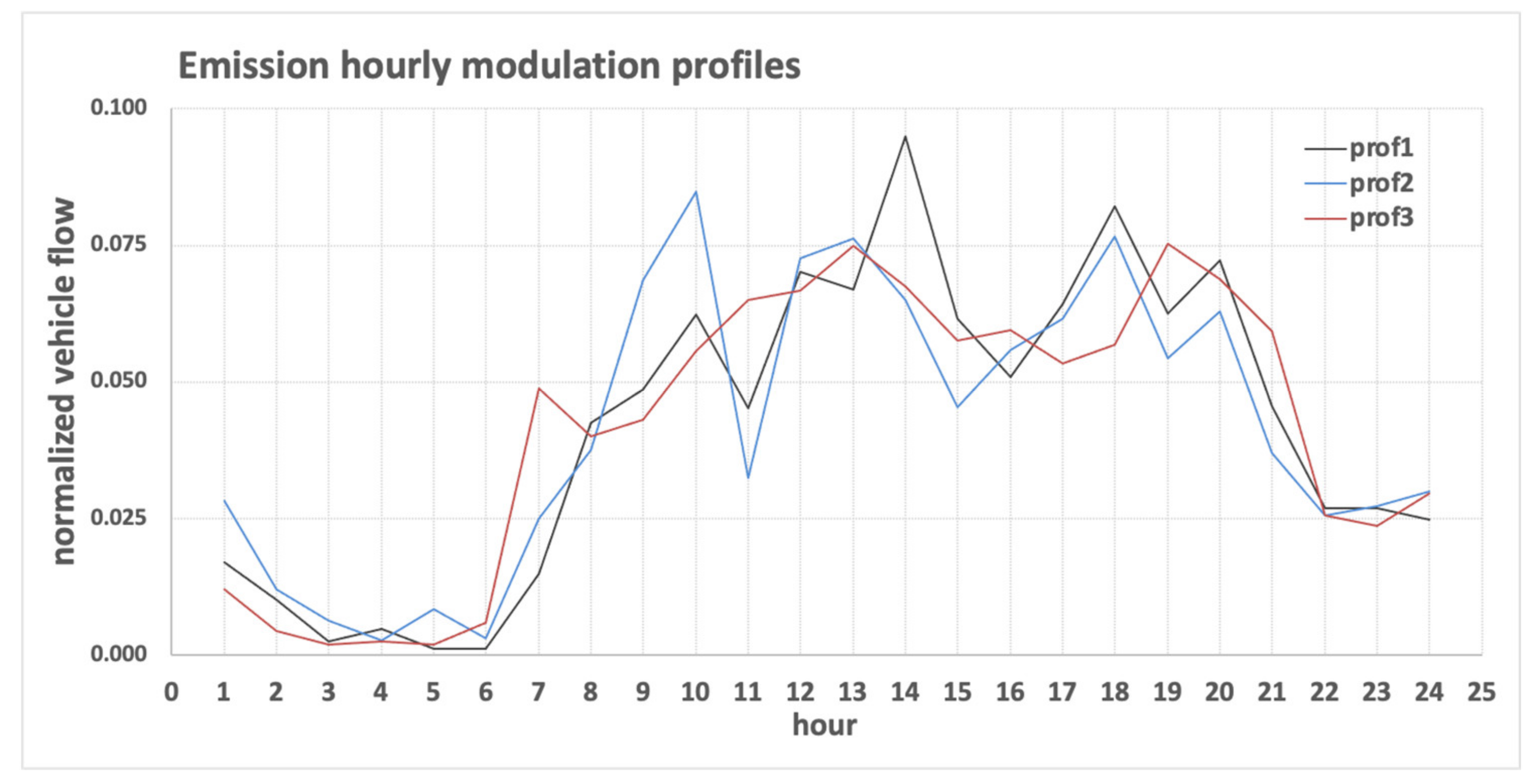
- Profile 1 (prof1): shows a steady increase in traffic from the very early morning to midday when it started decreasing more slowly than during the morning increase;
- -
- Profile 2 (prof2): shows 3 peaks, one in the morning at 10, one at 12–13, and the other at 18;
- -
- Profile 3 (prof3): shows two relevant peaks: one at 13 and the other at 18.
- -
- Sim 1: we used the passenger cars traffic fluxes from the FCD database, the modulation profiles described in Figure 4, and the relative percentages listed in Table 2 to calculate with TREFIC the traffic emissions due to passenger cars, motorcycles, heavy duty vehicles, and light duty vehicles to be used as input to PMSS;
- -
- Sim 2: this simulation was similar to Sim 1, and the calculation was performed only for passenger cars;
- -
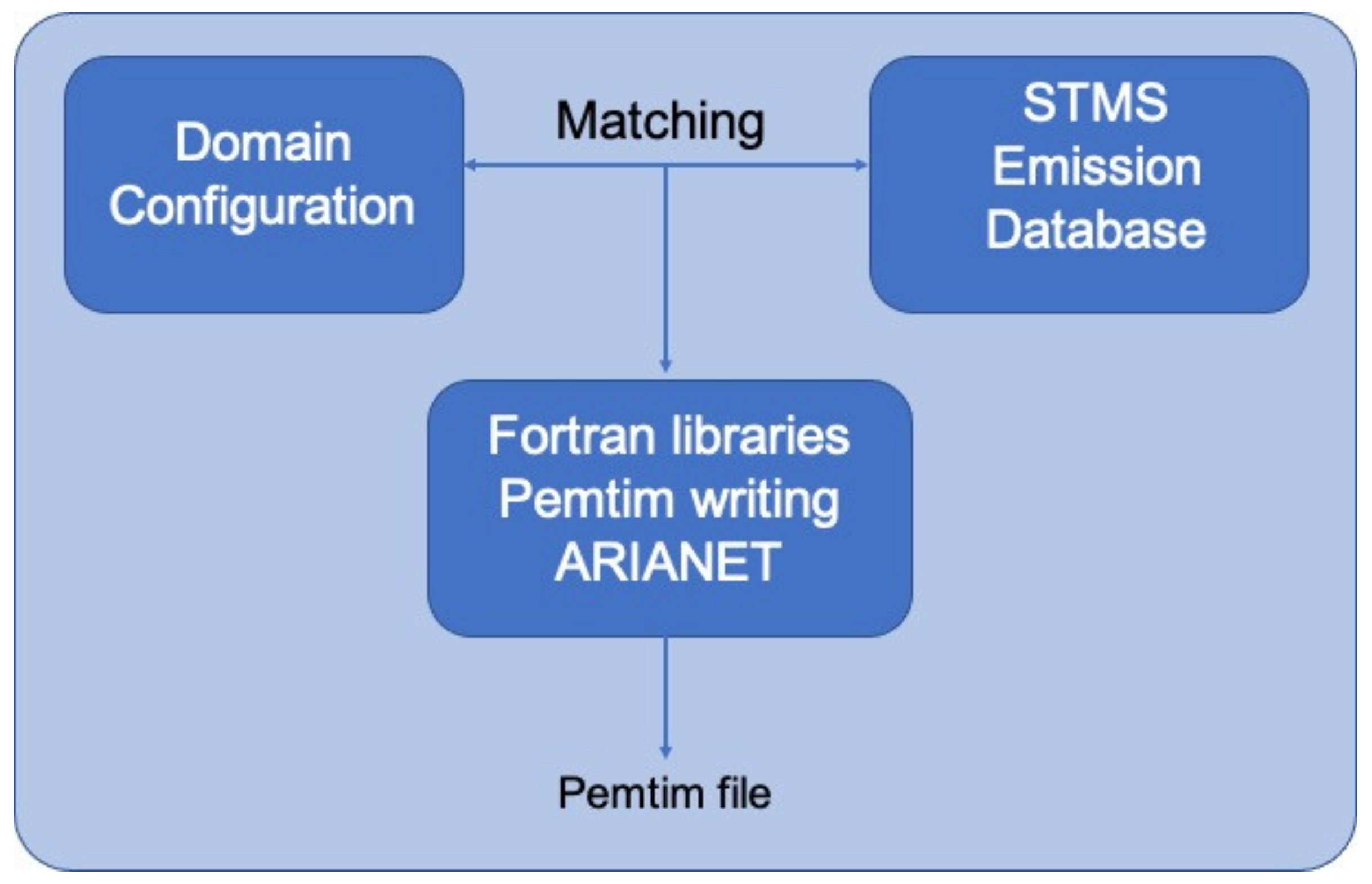
- Sim 3: we used as the input for PMSS the emissions already present in the FCD database in terms of emitted mass/unit time. These emissions were calculated using the emission processor ECOTRIP considering only passenger car traffic fluxes.
- The operation of translating fluxes into emissions was completed using two different traffic processors, which despite being both based on COPERT 4 methodologies, still showed some differences (not shown here);
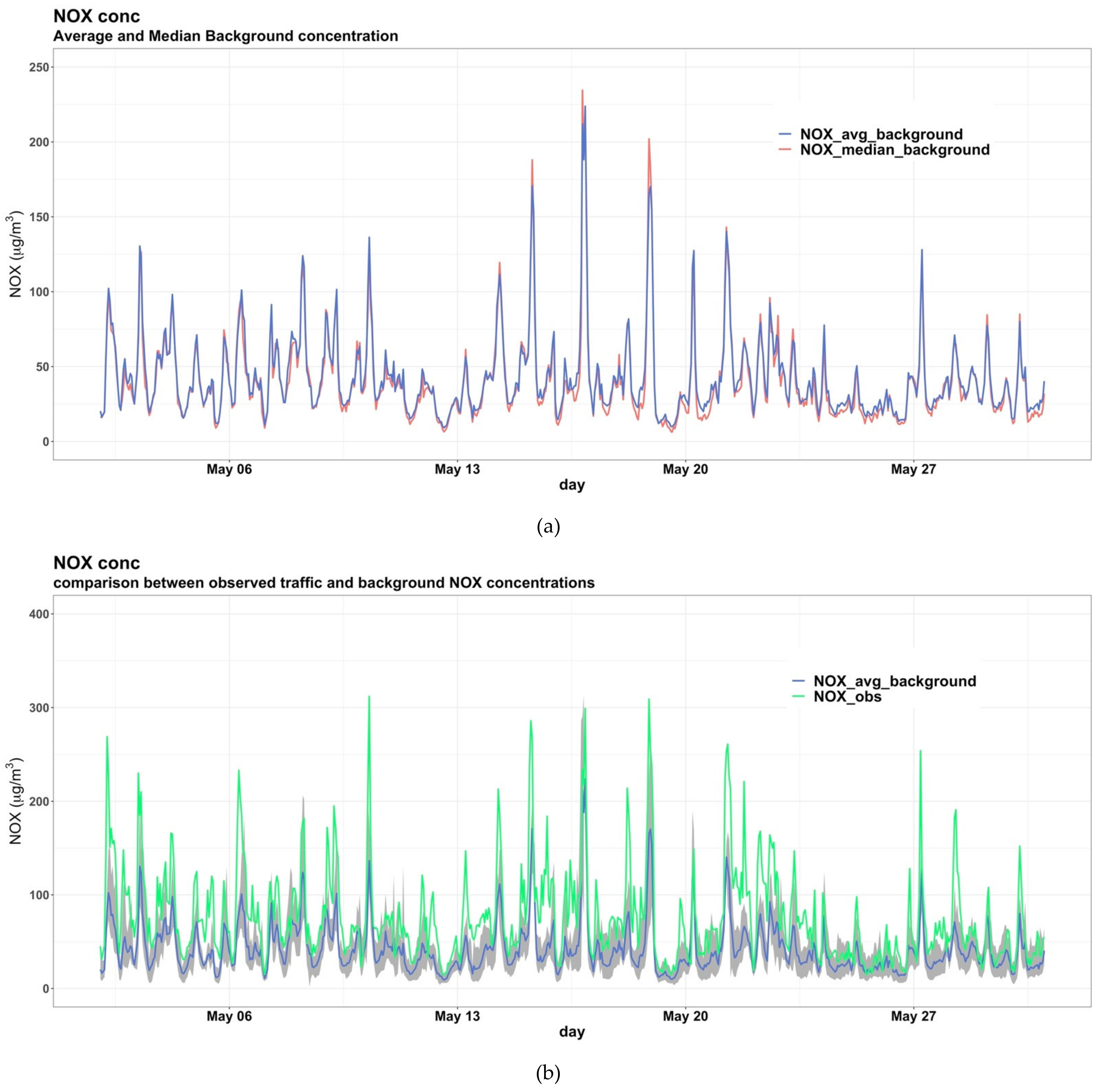
2.4.3. NOx Background
3. Results and Discussion
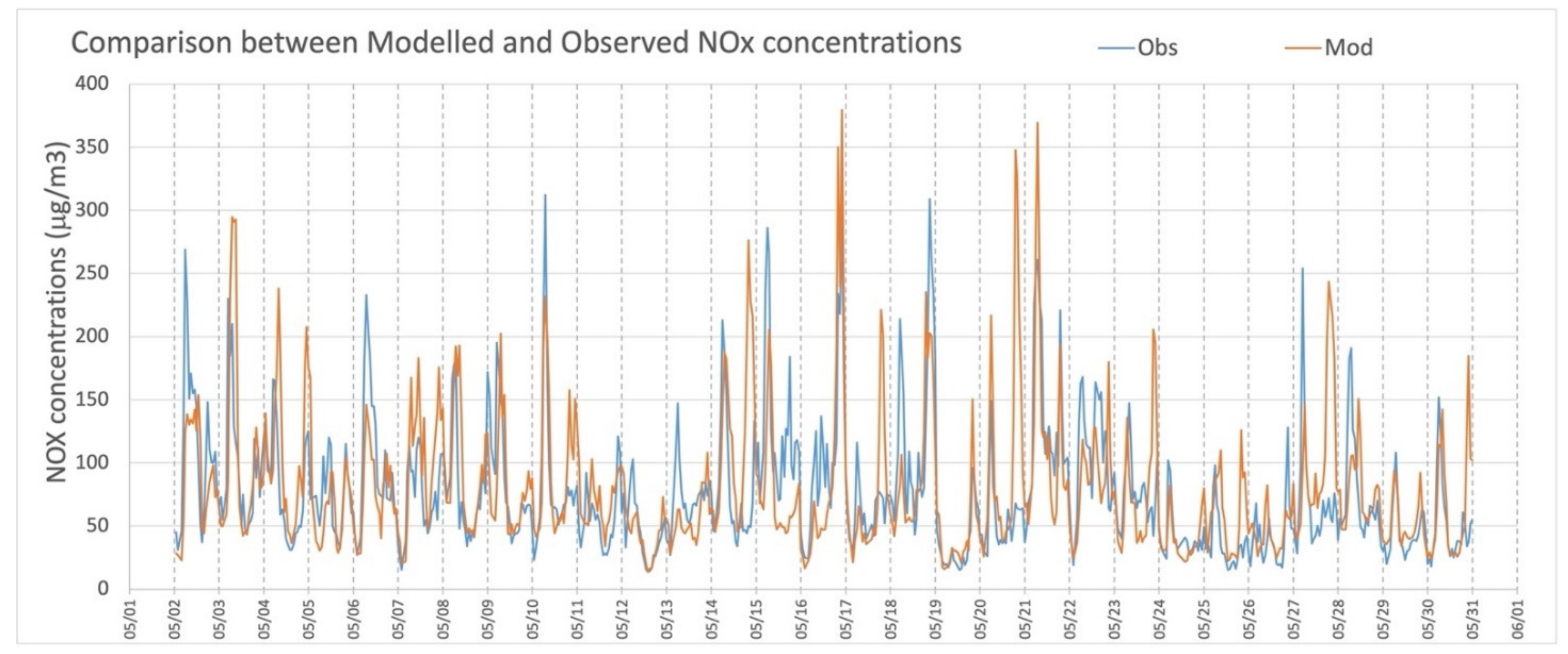
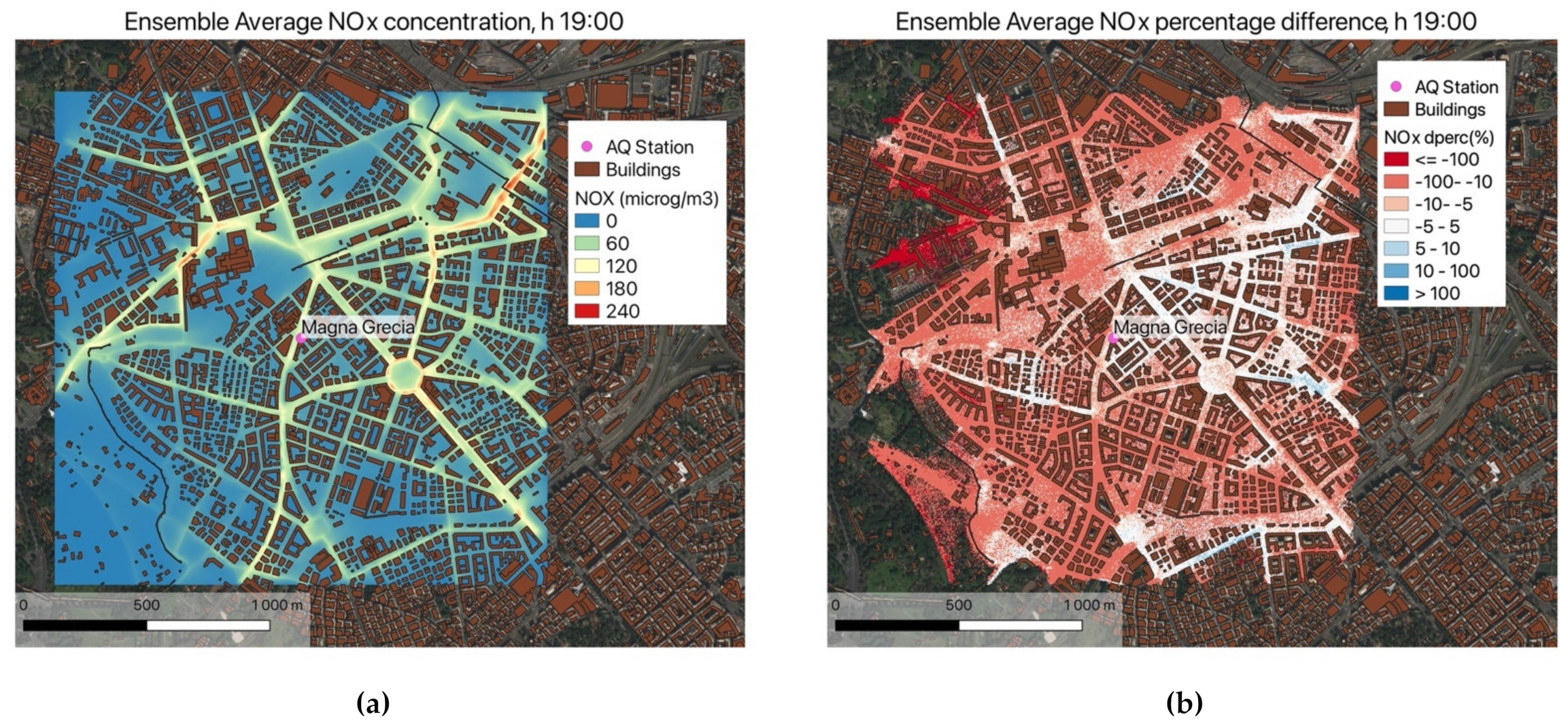
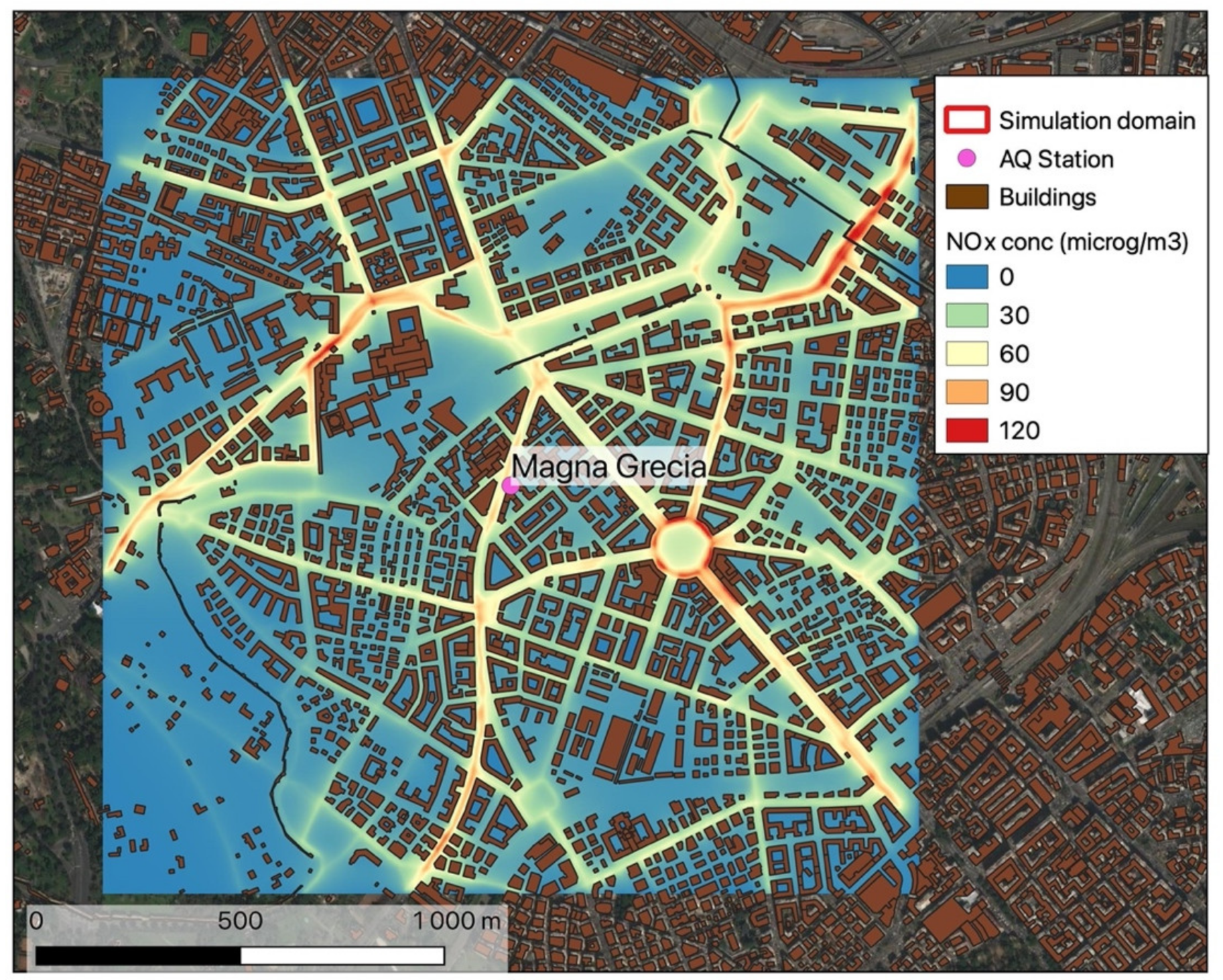
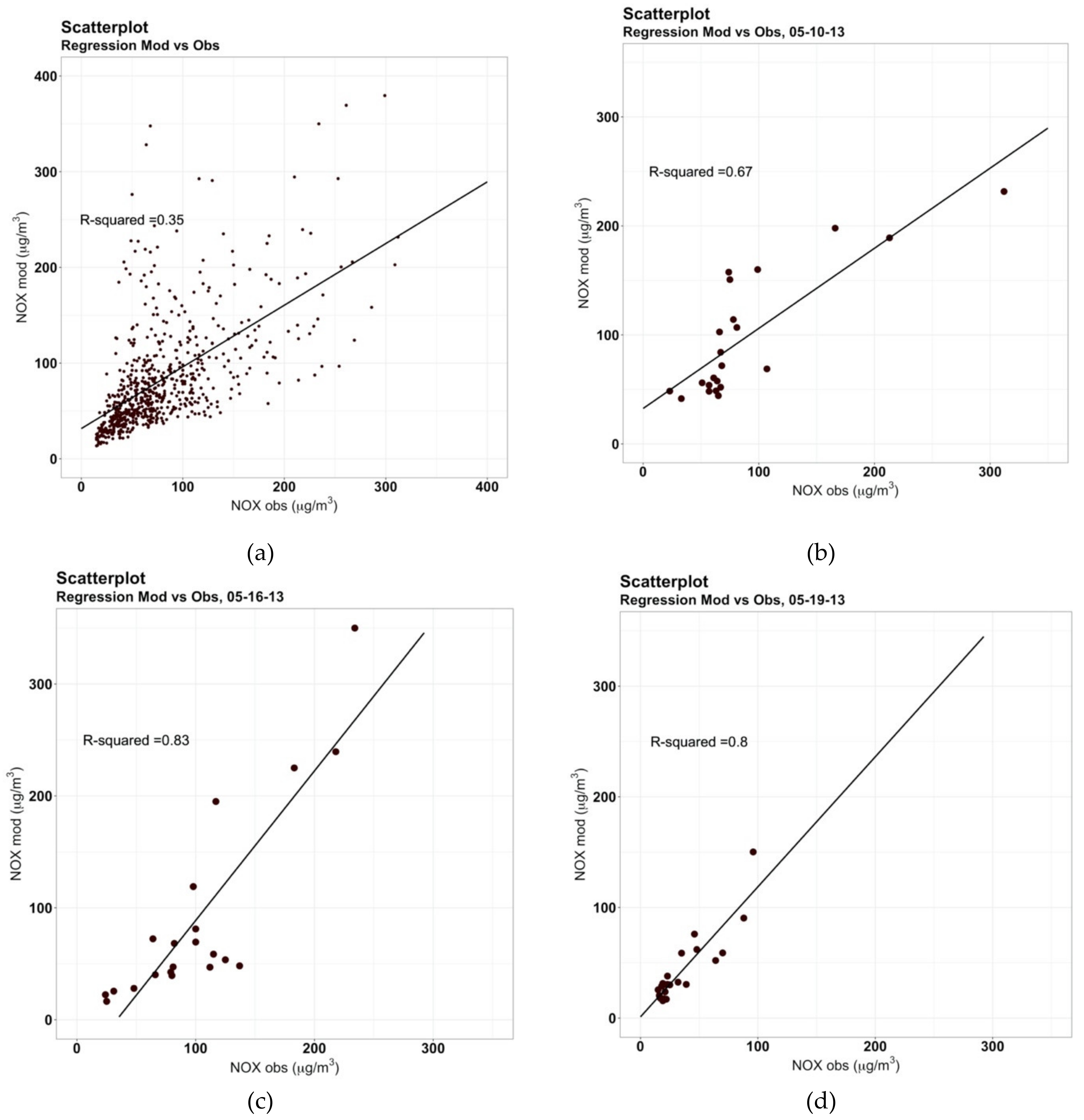
3.1. PMSS Traffic Emission Simulation (Sim 1)
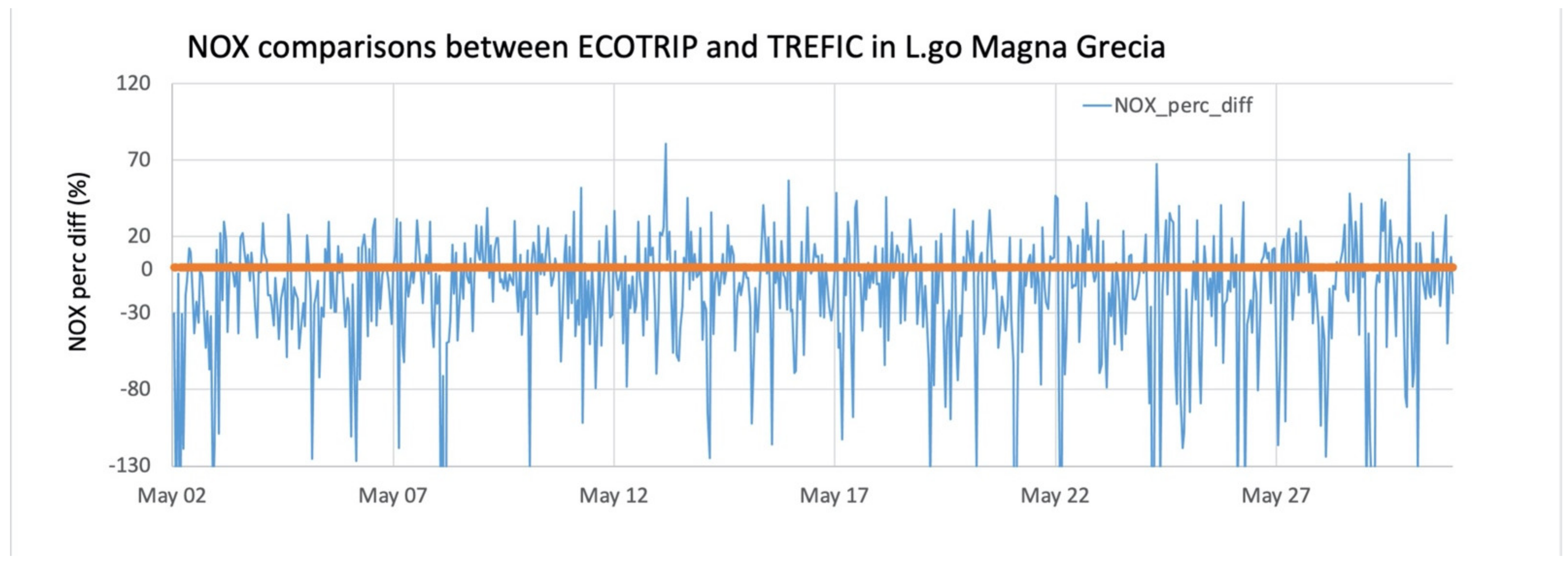
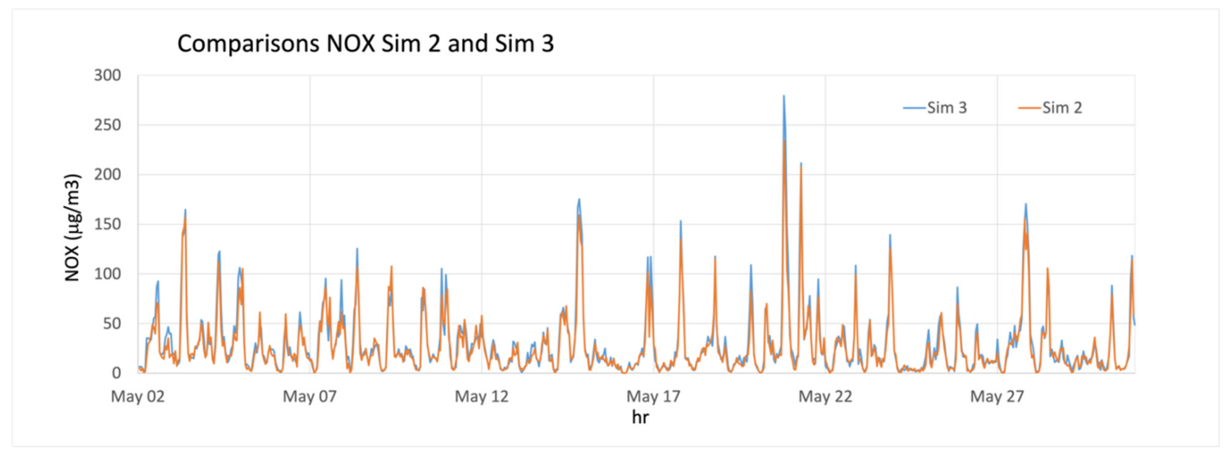
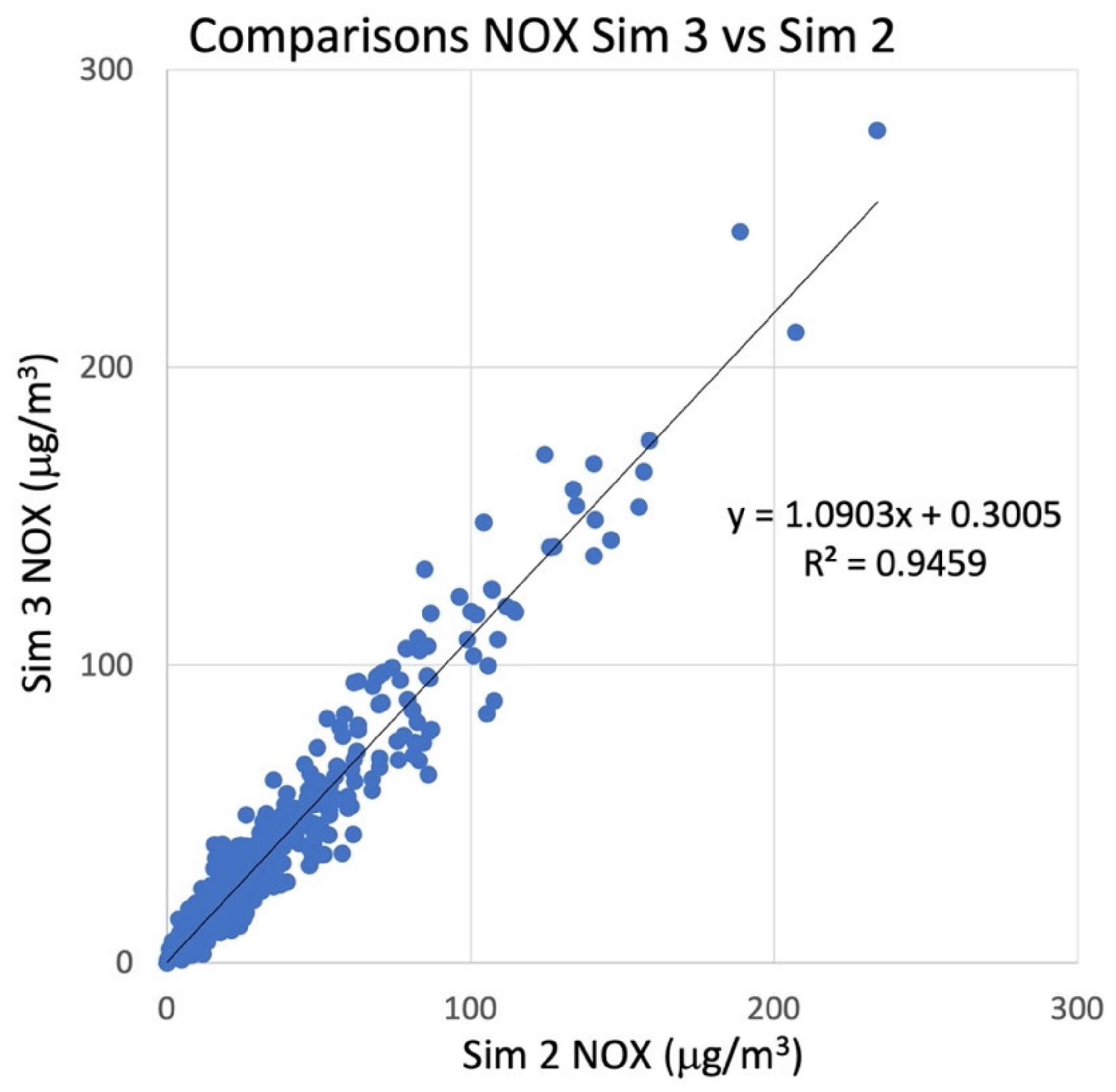
3.2. Comparison between Emission Processors (Sim 2 and Sim 3)
4. Conclusions
Author Contributions
Funding
Data Availability Statement
Acknowledgments
Conflicts of Interest
Appendix A
Appendix A.1. From ECOTRIP Data to PMSS Emission Input
Appendix A.2. Emission Processors Comparison

Appendix B

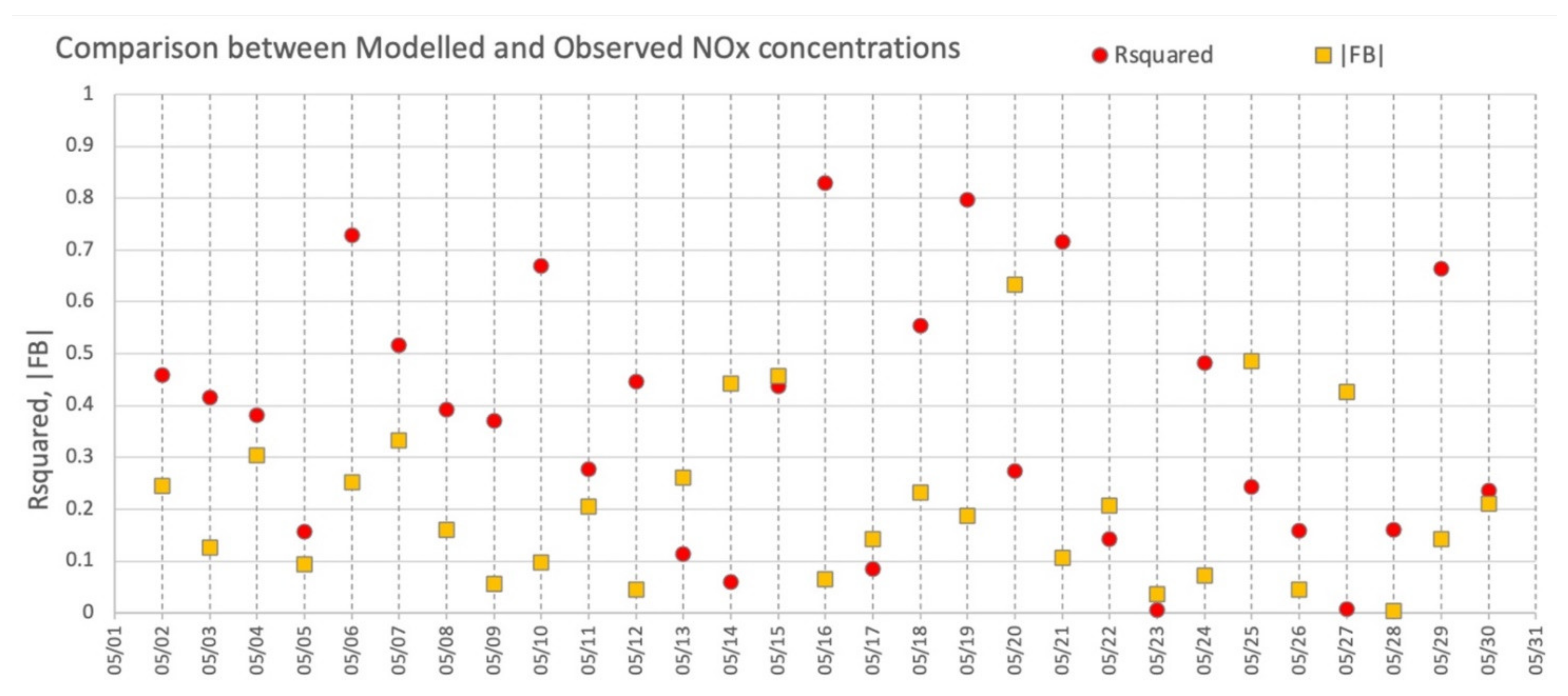
| Type of Measuring Station | |FB| | NMSE | FAC2 | NAD |
|---|---|---|---|---|
| Rural | |FB|≤0.3 | ≤3 | ≥0.5 | ≤0.3 |
| Urban | |FB|≤0.67 | ≤6 | ≥0.3 | ≤0.5 |
References
- Fenger, J. Urban air quality. Atmos. Environ. 1999, 33, 4877–4900. [Google Scholar] [CrossRef]
- Harrison, R.M.; Vu, T.V.; Jafar, H.; Shi, Z. More mileage in reducing urban air pollution from road traffic. Environ. Int. 2021, 149, 106329. [Google Scholar] [CrossRef]
- Marinello, S.; Lolli, F.; Gamberini, R. Roadway tunnels: A critical review of air pollutant concentrations and vehicular emissions. Transp. Res. D Transp. Environ. 2020, 86, 102478. [Google Scholar] [CrossRef]
- Hak, C.; Larssen, S.; Randall, S.; Guerreiro, C.; Denby, B.; Horálek, J. Traffic and Air Quality—Contribution of Traffic to Urban Air Quality in European Cities. ETC/ACC Technical Paper 2009/12, 2010. Available online: https://www.eionet.europa.eu/etcs/etc-atni/products/etc-atni-reports/etcacc_tp_2009_12_traffic_and_urban_air_quality (accessed on 25 March 2021).
- Vardoulakis, S.; Fisher, B.E.A.; Pericleous, K.; Gonzalez-Flesca, N. Modelling air quality in street canyons: A review. Atmos. Environ. 2003, 37, 155–182. [Google Scholar] [CrossRef] [Green Version]
- Huang, Y.; Lei, C.; Liu, C.; Perez, P.; Forehead, H.; Kong, S.; Zhou, J.L. A review of strategies for mitigating roadside air pollution in urban street canyons. Environ. Pollut. 2021, 280, 116971. [Google Scholar] [CrossRef] [PubMed]
- Wang, Y.; Szeto, W.Y.; Han, K.; Friesz, T.L. Dynamic traffic assignment: A review of the methodological advances for environmentally sustainable road transportation applications. Transp. Res. Part B Methodol. 2018, 111, 370–394. [Google Scholar] [CrossRef]
- El-Fadel, M.; Sbayti, H.; Kaysi, I. Modeling of Traffic-Induced Emission Inventories in Urban Areas. Effect of Roadway Network Aggregation Levels Traffic Management and Technology (2002). In Air Pollution Modelling and Simulation; Sportisse, B., Ed.; Springer: Berlin/Heidelberg, Germany, 2020. [Google Scholar] [CrossRef]
- Pinto, J.A.; Kumar, P.; Alonso, M.F.; Andreão, W.L.; Pedruzzi, R.; Dos Santos, F.; Moreira, D.M.; de Almeida Albuquerque, T.T. Traffic data in air quality modeling: A review of key variables, improvements in results, open problems and challenges in current research. Atmos. Pollut. Res. 2020, 11, 454–468. [Google Scholar] [CrossRef]
- Quaassdorff, C.; Borge, R.; Pérez, J.; Lumbreras, J.; de la Paz, D.; de Andrés, J.M. Microscale traffic simulation and emission estimation in a heavily trafficked roundabout in Madrid (Spain). Sci. Total Environ. 2016, 566–567, 416–427. [Google Scholar] [CrossRef] [PubMed]
- De Fabritiis, C.; Ragona, R.; Valenti, G. Traffic estimation and prediction based on real time floating car data. In Proceedings of the 11th International IEEE Conference on Intelligent Transportation Systems, Beijing, China, 12–15 October 2008; pp. 197–203. [Google Scholar]
- Karagulian, F.; Messina, G.; Valenti, G.; Liberto, C.; Carapellucci, F. A Simplified Map-Matching Algorithm for Floating Car Data. In Advanced Information Networking and Applications, AINA 2021, Lecture Notes in Networks and Systems; Barolli, L., Woungang, I., Enokido, T., Eds.; Springer: Cham, Switzerland, 2021; Volume 227. [Google Scholar] [CrossRef]
- Jing, B.; Wu, L.; Mao, H.; Gong, S.; He, J.; Zou, C.; Song, G.; Li, X.; Wu, Z. Development of a vehicle emission inventory with high temporal–spatial resolution based on NRT traffic data and its impact on air pollution in Beijing – Part 1: Development and evaluation of vehicle emission inventory. Atmos. Chem. Phys. 2016, 16, 3161–3170. [Google Scholar] [CrossRef] [Green Version]
- Gately, C.K.; Hutyra, L.R.; Peterson, S.; Wing, I.S. Urban emissions hotspots: Quantifying vehicle congestion and air pollution using mobile phone GPS data. Environ. Pollut. 2017, 229, 496–504. [Google Scholar] [CrossRef]
- Jiang, Y.; Song, G.; Zhang, Z.; Zhai, Z.; Yu, L. Estimation of Hourly Traffic Flows from Floating Car Data for Vehicle Emission Estimation. J. Adv. Transp. 2021, 2021, 6628335. [Google Scholar] [CrossRef]
- Iannone, F.; Ambrosino, F.; Bracco, G.; De Rosa, M.; Funel, A.; Guarnieri, G.; Migliori, S.; Palombi, F.; Ponti, G.; Santomauro, G.; et al. CRESCO ENEA HPC clusters: A working example of a multifabric GPFS Spectrum Scale layout. In Proceedings of the 2019 International Conference on High Performance Computing Simulation (HPCS), Dublin, Ireland, 15–19 July 2019; pp. 1051–1052. [Google Scholar] [CrossRef]
- Mastroianni, P.; Monechi, B.; Servedio, V.; Liberto, C.; Valenti, G.; Loreto, V. Individual Mobility Patterns in Urban Environment. In Proceedings of the 1st International Conference on Complex Information Systems, Rome, Italy, 22–25 April 2016; pp. 81–88. [Google Scholar] [CrossRef] [Green Version]
- Altintasi, O.; Tuydes-Yaman, H.; Tuncay, K. Detection of urban traffic patterns from Floating Car Data (FCD). Transp. Res. Procedia. 2017, 22, 382–391. [Google Scholar] [CrossRef]
- Mastroianni, P.; Monechi, B.; Liberto, C.; Valenti, G.; Servedio, V.D.P.; Loreto, V. Local Optimization Strategies in Urban Vehicular Mobility. PLoS ONE 2015, 10, e0143799. [Google Scholar] [CrossRef] [Green Version]
- Dölger, R.; Kleine, S.; Hoffmann, T.; Schreuder, M.; Ferrante, E.; Pressi, F.; Kaltwasser, J.; Ansorge, J.; Haspel, U.; Cheung, S.; et al. Floating Car Data, Report v. 01-00-00, FCD Workshop, Frankfurt 17th September 2019. Available online: https://www.its-platform.eu/filedepot_download/2218/6585 (accessed on 31 July 2021).
- Cohn, N.; Bischoff, H. Floating Car Data for Transportation Planning: Explorative Study to Technique and Applications and Sample Properties of GPS Data, TomTom Presentation Slides, NATMEC, Dallas. 2012. Available online: http://onlinepubs.trb.org/onlinepubs/conferences/2012/NATMEC/Cohn.pdf (accessed on 31 July 2021).
- Liberto, C.; Ragona, R.; Valenti, G. Traffic Prediction in Metropolitan Freeways. In Proceedings of the 7th International Conference on Traffic & Transportation Studies, ICTTS, Kunming, China, 3–5 August 2010; pp. 846–860, vol: Traffic and Transportation Studies, 2010. [Google Scholar] [CrossRef]
- Ehmke, J.F.; Meisel, S.; Mattfeld, D.C. Floating Car Data Based Analysis of Urban Travel Times for the Provision of Traffic Quality. In Traffic Data Collection and Its Standardization; International Series in Operations Research & Management Science; Barceló, J., Kuwahara, M., Eds.; Springer: New York, NY, USA, 2010; Volume 144. [Google Scholar] [CrossRef]
- Brockfeld, E.; Lorkowski, S.; Mieth, P.; Wagner, P. Benefits and Limits of Recent Floating Car Data Technology—An Evaluation Study. In Proceedings of the 11th WCTR Conference, Berkeley, CA, USA, 24–28 June 2007. [Google Scholar]
- Leduc, G. Road Traffic Data: Collection Methods and Applications. Work. Pap. Energy Transp. Clim. Chang. 2008, 1, 1–55. [Google Scholar]
- Octo Telematics Website. Available online: https://www.octotelematics.com/company/ (accessed on 9 May 2021).
- Nigro, M.; Ferrara, M.; De Vincentis, R.; Liberto, C.; Valenti, G. Data Driven Approaches for Sustainable Development of E-Mobility in Urban Areas. Energies 2021, 14, 3949. [Google Scholar] [CrossRef]
- Lelli, M.; Liberto, C.; Valenti, G. Aggiornamento delle Librerie Software “ECOTRIP” per la Stima dei Consumi e delle Emissioni, Contratto di Servizio Tecnico-Scientifico tra ENEA e OctoTelematics SpA, Det. n.18/E/2016/DTE, C.A. CT4AAC; ENEA e OctoTelematics SpA: Rome, Italy, 2017. [Google Scholar]
- ARIANET. TREFIC—Traffic Emission Factors Improved Calculator. 2014. Available online: http://www.aria-net.it/front/ENG/codes/files/7.pdf (accessed on 19 April 2021).
- Emisia SA. COPERT—COmputer Programme to Calculate Emissions from Road Transport. 2018. Available online: https://www.emisia.com/utilities/copert/documentation (accessed on 11 June 2020).
- Liberto, C.; Valenti, G.; Orchi, S.; Lelli, M.; Nigro, M.; Ferrara, M. The Impact of Electric Mobility Scenarios in Large Urban Areas: The Rome Case Study. IEEE Trans. Intell. Transp. Syst. 2018, 19, 3540–3549. [Google Scholar] [CrossRef]
- Valenti, G.; Lelli, M.; Liberto, C.; Orchi, S.; Messina, G.; Ortenzi, F.; Carapellucci, F. Valutazione dei benefici ambientali della mobilità elettrica nell’area di Roma, Report Ricerca di Sistema Elettrico. RdS/PAR2015/213; ENEA: Rome, Italy, 2016. (In Italian) [Google Scholar]
- Ntziachristos, L.; Samaras, Z. EMEP/EEA Air Pollutant Emission Inventory Guidebook 2016, in 1.A.3.b.i-iv (Passenger Cars, Light Commercial Trucks, Heavy-Duty Vehicles Including Buses and Motor Cycles). June 2017. Available online: http://www.eea.europa.eu/publications/emep-eea-guidebook-2016/part-b-sectoral-guidancechapters/1-energy/1-a-combustion/1-a-3-b-i (accessed on 20 May 2017).
- Joumard, R.; Andre, J.M.; Rapone, M.; Zallinger, M.; Kljun, N.; Andre, M.; Samaras, Z.; Roujol, S.; Laurikko, J.; Weilenmann, M. Emission Factor Modelling and Database for Light Vehicles—Artemis Deliverable 3, Document LTE 0523. 2007. Available online: http://hal.archives-ouvertes.fr/hal-00916945/document (accessed on 12 April 2017).
- Oldrini, O.; Armand, P.; Duchenne, C.; Olry, C.; Moussafir, J.; Tinarelli, G. Description and Preliminary Validation of the PMSS Fast Response Parallel Atmospheric Flow and Dispersion Solver in Complex Built-Up Areas, Environ. Fluid Mech. 2017, 17, 997–1014. [Google Scholar] [CrossRef]
- Tinarelli, G.; Mortarini, L.; Trini Castelli, S.; Carlino, G.; Moussafir, J.; Olry, C.; Armand, P.; Anfossi, D. Review and Validation of Microspray, a Lagrangian Particle Model of Turbulent Dispersion. Geophys. Monogr. Ser. 2012, 200, 311–327. [Google Scholar] [CrossRef]
- Tinarelli, G.; Gomez, F. PSPRAY General Description and User’s Guide, 2017. Version Code 3.7.3.; ARIANET/ARIA Technologies: Milan, Italy, 2017. [Google Scholar]
- Nibart, M.; Armand, P.; Duchenne, C.; Olry, C.; Albergel, A.; Moussafir, J.; Oldrini, O. Flow and Dispersion Modelling in a Complex Urban District Taking account of the Underground Roads Connections. In Proceedings of the 17th International Conference on Harmonization within Atmospheric Dispersion Modelling for Regulatory Purposes, Budapest, Hungary, 9–12 May 2016. [Google Scholar]
- Finardi, S.; Silibello, C. SURFPRO3 User’s Guide (SURFace-Atmosphere Interface PROcessor, Version 3); Software Manual. Arianet R2011.31; Arianet: Milan, Italy. 2011. Available online: http://doc.aria-net.it/SURFPRO (accessed on 17 August 2021).
- Finardi, S.; Morselli, M.G.; Brusasca, G.; Tinarelli, G. A 2-D meteorological pre-processor for real-time 3-D ATD models. Int. J. Environ. Pollut. 1997, 8, 478–488. [Google Scholar]
- ARIANET. ARIA(NET). Available online: http://www.aria-net.it/ (accessed on 20 April 2020).
- Skamarock, W.C.; Klemp, J.B.; Dudhia, J.; Gill, D.O.; Barker, D.M.; Duda, M.G.; Huang, X.-Y.; Wang, W.; Powers, J.G. A Description of the Advanced Research WRF Version 3. NCAR Tech. Note 2008, NCAR/TN-475+STR; University Corporation for Atmospheric Research: Boulder, CO, USA, 2008; 113p. [Google Scholar]
- Hersbach, H.; Bell, B.; Berrisford, P.; Hirahara, S.; Horányi, A.; Muñoz-Sabater, J.; Nicolas, J.; Peubey, C.; Radu, R.; Schepers, D.; et al. The ERA5 global reanalisys. Q. J. R. Met. Soc. 2020, 146, 1999–2049. [Google Scholar] [CrossRef]
- Hong, S.-Y.; Dudhia, J.; Chen, S.-H. A revised approach to ice microphysical processes for the bulk parameterization of clouds and precipitation. Mon. Weather Rev. 2004, 132, 103–120. [Google Scholar] [CrossRef]
- Dudhia, J. Numerical study of convection observed during the Winter Monsoon Experiment using a mesoscale two–dimensional model. J. Atmos. Sci. 1989, 46, 3077–3107. [Google Scholar] [CrossRef]
- Mlawer, E.J.; Taubman, S.J.; Brown, P.D.; Iacono, M.J.; Clough, S.A. Radiative transfer for inhomogeneous atmospheres: RRTM, a validated correlated–k model for the longwave. J. Geophys. Res. 1997, 102, 16663–16682. [Google Scholar] [CrossRef] [Green Version]
- Jimenez, P.A.; Dudhia, J.; Gonzalez–Rouco, J.F.; Navarro, J.; Montavez, J.P.; Garcia–Bustamante, E. A revised scheme for the WRF surface layer formulation. Mon. Weather Rev. 2012, 140, 898–918. [Google Scholar] [CrossRef] [Green Version]
- Tewari, M.; Chen, F.; Wang, W.; Dudhia, J.; LeMone, M.A.; Mitchell, K.; Ek, M.; Gayno, G.; Wegiel, J.; Cuenca, R.H. Implementation and verification of the unified NOAH land surface model in the WRF model. In Proceedings of the 20th Conference on Weather Analysis and Forecasting/16th Conference on Numerical Weather Prediction, Seattle, WA, USA, 12–16 January 2004; pp. 11–15. [Google Scholar]
- Hong, S.-Y.; Noh, Y.; Dudhia, J. A new vertical diffusion package with an explicit treatment of entrainment processes. Mon. Weather Rev. 2006, 134, 2318–2341. [Google Scholar] [CrossRef] [Green Version]
- Kain, J.S. The Kain–Fritsch convective parameterization: An update. J. Appl. Meteor. 2004, 43, 170–181. [Google Scholar] [CrossRef] [Green Version]
- ACI. Available online: http://www.aci.it/laci/studi-e-ricerche/dati-e-statistiche.html (accessed on 29 March 2021).
- Ghermandi, G.; Fabbi, S.; Baranzoni, G.; Veratti, G.; Bigi, A.; Teggi, S.; Barbieri, C.; Torreggiani, L. Vehicular exhaust impact simulated at microscale from traffic flow automatic surveys and emission factor evaluation. In Proceedings of the 18th International Conference on Harmonisation within Atmospheric Dispersion Modelling for Regulatory Purposes, HARMO 2017, Bologna, Italy, 9–12 October 2017; Volume 2017, pp. 475–479. [Google Scholar]
- Sanchez, B.; Santiago, J.L.; Martilli, A.; Martin, F.; Borge, R.; Quaassdorff, C.; de la Paz, D. Modelling NOX concentrations through CFD-RANS in an urban hot-spot using high resolution traffic emissions and meteorology from a mesoscale model. Atmos. Environ. 2017, 163, 155–165. [Google Scholar] [CrossRef]
- Air Quality e-Reporting (AQ e-Reporting), European Environmental Agency. Available online: httos://www.eea.europa.eu/data-and-maps/data/aqereporting-2 (accessed on 9 May 2021).
- The R Base Package. Available online: https://www.rdocumentation.org/packages/base/versions/3.6.2 (accessed on 21 August 2020).
- The R Lubridate Package: Make Dealing with Dates a Little Easier. Available online: https://cran.r-project.org/web/packages/lubridate/index.html (accessed on 28 August 2020).
- The Rrgdal Package: Bindings for the ‘Geospatial’ Data Abstraction Library. Available online: https://cran.r-project.org/web/packages/rgdal/index.html (accessed on 28 August 2020).
- Janssen, S.; Thunis, P. FAIRMODE Guidance Document on Modelling Quality Objectives and Benchmarking; EUR 30264 EN; Publications Office of the European Union: Luxembourg, 2020; JRC120649; ISBN 978-92-76-19746-1. [Google Scholar] [CrossRef]
- Hanna, S.; Chang, J. Acceptance criteria for urban dispersion model evaluation. Meteor. Atmos. Phys. 2012, 116, 133–146. [Google Scholar] [CrossRef]
- Ghermandi, G.; Fabbri, S.; Veratti, G.; Bigi, A.; Teggi, S. Estimate of Secondary NO2 Levels at Two Urban Traffic Sites Using Observations and Modelling. Sustainability 2020, 12, 7897. [Google Scholar] [CrossRef]
- Villani, M.G.; Russo, F.; Adani, M.; Piersanti, A.; Vitali, L.; Tinarelli, G.; Ciancarella, L.; Zanini, G.; Donateo, A.; Rinaldi, M.; et al. Evaluating the Impact of a Wall-Type Green Infrastructure on PM10 and NOx Concentrations in an Urban Street Environment. Atmosphere 2021, 12, 839. [Google Scholar] [CrossRef]
- Best, D.J.; Roberts, D.E. Algorithm AS 89: The Upper Tail Probabilities of Spearman’s Rho. Appl. Stat. 1975, 24, 377–379. [Google Scholar] [CrossRef]
- Hollander, M.; Wolfe, D.A. Nonparametric Statistical Methods; John Wiley & Sons: New York, NY, USA, 1973; pp. 185–194. [Google Scholar]


| Parameterization | Reference |
|---|---|
| Cloud microphysics | Hong et al., 2004 [44] |
| Short wave radiation | Dudhia, 1989 [45] |
| Long wave radiation | Mlawer, 1997 [46] |
| Surface layer | Jimenez et al., 2012 [47] |
| Land surface model | Tewari et al., 2004 [48] |
| Planetary boundary layer | Hong et al., 2006 [49] |
| Cumulus convection (activated over coarse domain only) | Kain, 2004 [50] |
| Vehicle Type | Fleet Composition |
|---|---|
| Passenger cars | 77.3% |
| Motorcycles | 17% |
| Light duty vehicles | 5.4% |
| Heavy duty vehicles | 0.3% |
| Profile ID | Vehicle Flux (Ftot) Range |
|---|---|
| 1 | Ftot < 3000 |
| 2 | 4000 < Ftot < 6000 |
| 3 | 6000 < Ftot < 11000 |
| Simulation Name | Type of Vehicle | Emission Processor |
|---|---|---|
| Sim 1 | Passenger cars Motorcycles Light duty Heavy duty | TREFIC |
| Sim 2 | Passenger cars | TREFIC |
| Sim 3 | Passenger cars | ECOTRIP |
| |FB| | NMSE | FAC2 | NAD | |
|---|---|---|---|---|
| Magna Grecia (Urban) | 0.049 | 0.37 | 0.87 | 0.20 |
Publisher’s Note: MDPI stays neutral with regard to jurisdictional claims in published maps and institutional affiliations. |
© 2021 by the authors. Licensee MDPI, Basel, Switzerland. This article is an open access article distributed under the terms and conditions of the Creative Commons Attribution (CC BY) license (https://creativecommons.org/licenses/by/4.0/).
Share and Cite
Russo, F.; Villani, M.G.; D’Elia, I.; D’Isidoro, M.; Liberto, C.; Piersanti, A.; Tinarelli, G.; Valenti, G.; Ciancarella, L. A Study of Traffic Emissions Based on Floating Car Data for Urban Scale Air Quality Applications. Atmosphere 2021, 12, 1064. https://doi.org/10.3390/atmos12081064
Russo F, Villani MG, D’Elia I, D’Isidoro M, Liberto C, Piersanti A, Tinarelli G, Valenti G, Ciancarella L. A Study of Traffic Emissions Based on Floating Car Data for Urban Scale Air Quality Applications. Atmosphere. 2021; 12(8):1064. https://doi.org/10.3390/atmos12081064
Chicago/Turabian StyleRusso, Felicita, Maria Gabriella Villani, Ilaria D’Elia, Massimo D’Isidoro, Carlo Liberto, Antonio Piersanti, Gianni Tinarelli, Gaetano Valenti, and Luisella Ciancarella. 2021. "A Study of Traffic Emissions Based on Floating Car Data for Urban Scale Air Quality Applications" Atmosphere 12, no. 8: 1064. https://doi.org/10.3390/atmos12081064
APA StyleRusso, F., Villani, M. G., D’Elia, I., D’Isidoro, M., Liberto, C., Piersanti, A., Tinarelli, G., Valenti, G., & Ciancarella, L. (2021). A Study of Traffic Emissions Based on Floating Car Data for Urban Scale Air Quality Applications. Atmosphere, 12(8), 1064. https://doi.org/10.3390/atmos12081064