Article

Total Ozone Trends in East Asia from Long-Term Satellite and Ground Observations

1
National Institute of Meteorological Sciences, Seogwipo-si 63568, Korea
2
Department of Atmospheric Sciences, Yonsei University, Seoul 03722, Korea
*
Author to whom correspondence should be addressed.
Atmosphere 2021, 12(8), 982; https://doi.org/10.3390/atmos12080982
Submission received: 23 June 2021 / Revised: 16 July 2021 / Accepted: 26 July 2021 / Published: 29 July 2021
(This article belongs to the Special Issue Wintertime Urban Photochemical Air Pollution in Asia)

Abstract

:
The ozone concentration in the atmosphere has been recovering with the reduction in atmospheric ozone-depleting substances (ODS). However, ODS remain in the atmosphere for long periods, slowing recovery. Furthermore, greenhouse gas-induced climate change complicates ozone recovery. East Asia is a significant contributor to global climate change due to the increase in industrialization and the presence of complex climate conditions. We investigated ozone variations in East Asia using total column ozone data based on satellite and ground observations and compared the results and trends derived from a multi-linear regression (MLR) model. We found that the MLR model has relatively poor explanatory power for recent extraterrestrial and dynamical proxies, but the uncertainty can be reduced using monthly data and atmospheric proxies. The ozone trend in East Asia had the greatest increase in the vicinity of the Korean Peninsula and Manchuria from 1997 to 2017 (~1% per decade). Similarly, the trend derived from Brewer spectrophotometer data was 1.02 ± 1.45% per decade in Pohang and 1.27 ± 0.85% per decade in Seoul. When the analysis period was extended to 2020, the impact of atmospheric variability was greater, suggesting that recent climate change can increasingly contribute to total ozone variability.

1. Introduction

The importance of ozone in the atmosphere has been widely known to the public since the discovery of the Antarctic ozone hole in the mid-1980s. The ozone hole posed a direct threat to the survival of humans living on Earth, and the Montreal Protocol was quickly adopted in 1987 in response to this. As a result, chlorofluorocarbon (CFC) emissions were highly constrained, and global ozone concentrations reached a significant turning point. Globally, the total column ozone first showed signs of recovery around the mid-1990s, but recovery has maintained a slow rate because ozone-depleting substances (ODS) are mostly stable and remain in the atmosphere for a long period [1,2,3,4,5]. In addition, climate change, caused by increases in greenhouse gases (GHGs) levels, has increased the uncertainty regarding recent changes in ozone concentrations [6,7,8].
Ozone destruction in the stratosphere occurs through catalytic chemistry when ODS reach the stratosphere [9,10], which is affected not only by the amount of ODS but also by atmospheric conditions such as temperature [11,12]. In addition, climate change significantly affects ozone because it circulates globally via atmospheric circulation and can be locally transported by synoptic weather systems, which are impacted by climate change [13,14,15,16]. Moreover, the factors that can affect atmospheric ozone concentration are highly diverse; some interact with each other, rendering it difficult to clearly account for ozone variations. However, from a long-term perspective, changes in the ozone concentration due to anthropogenic factors (i.e., ODS) are nearly linear, while changes due to natural variability, such as solar activity, quasi-biennial oscillation (QBO), aerosol optical depth (AOD), El Niño–Southern Oscillation (ENSO), and Arctic Oscillation (AO), usually have periodicity. Therefore, long-term analyses of ozone concentration mainly focus on linear, rather than periodic, trends, which are highly consistent with changes in the equivalent effective stratospheric chlorine (EESC), a parameter that can quantify the effects of halogens on ozone depletion in the stratosphere [17,18]. A multi-linear regression (MLR) analysis can explain the changes in ozone concentration based on the explanatory variables that affect ozone; this can provide linear trends that can be mainly attributed to anthropogenic activities.
Previous studies have analyzed long-term ozone change. Furthermore, the Ozone Assessment Report [2] and the SPARC/IO3C/GAW Report on Long-term Ozone Trends and Uncertainties in the Stratosphere (LOTUS) [3] comprehensively summarize related studies. According to the results of these studies, the change in total column ozone since the Montreal Protocol was most rapid in the Antarctic and has remained almost unchanged in the tropics. Prior to the turnaround point of the ODS concentration (in approximately 1997), a latitudinal dependence for the total ozone trend was observed, with ozone decreasing significantly at higher latitudes. After the turnaround point, this latitudinal dependence was not clearly observed [2,3,4,7]. Although the exact altitude differs depending on the data used for analysis, ozone recovery is most pronounced in the upper stratosphere (30–50 km); however, large uncertainty remains over the upper troposphere/lower stratosphere [3]. Following the Montreal Protocol, the recovery of the total column ozone began around 1997 in most regions, such that it is expected to return to the 1980 level within a few decades [19]. Nonetheless, the actual recovery of ozone concentration has been delayed with respect to the initial expectations owing to changes in GHG and ODS scenarios; considerable uncertainty still exists as to when the 1980 level will be reached [2,20].
Prior studies related to ozone trends have primarily focused on global changes. However, as the ozone concentration varies greatly depending on the regional climate and amount of precursors, the difference in trends between regions is quite large. East Asia is an important region for predicting and responding to future ozone levels because the atmospheric dynamics of the region are significant, and a substantial amount of pollutants has been released owing to ongoing rapid industrialization. In particular, factors such as changes in the general atmospheric circulation [21,22] and unexpected additional CFC emissions detected in China [23,24,25] have further increased the uncertainty in the recent ozone trend. Moreover, as the first geostationary orbit satellite GK-2B, equipped with a Geostationary Environment Monitoring Spectrometer (GEMS) environmental sensor, was recently successfully launched [26] with scheduled intensive ozone observations in East Asia, fundamental research is required to understand the characteristics of ozone variations in the East Asia region from the past to the present. Studies related to the long-term ozone trend in East Asia have been conducted using data on the total column ozone in Seoul or vertical ozone profiles in Pohang [14,16,27,28]. Nevertheless, studies on recent trends and overall changes in the East Asia region as a whole are still insufficient when compared with their importance.
In this study, total ozone trends in East Asia were investigated using MLR analysis. Furthermore, the trend uncertainty according to the time interval of time series data and the inclusion of atmospheric proxies was quantitatively compared. Through these analyses, we aimed to examine the recent characteristics of total ozone variation in East Asia and to suggest an analysis method suitable for recent trend analyses of regional-scale ozone fluctuations. This study is organized as follows: Section 2 describes the method and data used in this study. Section 3.1 compares the total ozone variability between East Asia and other latitude regions. Additionally, the difference in ozone variability before and after 1997 was examined. Section 3.2 analyzes the trend uncertainty according to atmospheric proxies, and Section 3.3 suggests the recent trends and uncertainty of total column ozone over East Asia. Lastly, Section 4 concludes the overall contents of this study and provides the direction of further research.

2. Materials and Methods

2.1. Satellite Composite Data

The solar backscattered ultraviolet (SBUV) observation system is a series of instruments that retrieve ozone from the surface to the uppermost atmosphere by observing nadir backscatter ultraviolet (UV) radiation. The National Aeronautics and Space Administration (NASA) provides SBUV merged ozone datasets (MOD), which is a monthly mean zonal and gridded average product, produced by merging individual SBUV/SBUV-2 satellite datasets [29,30,31,32]. SBUV MOD have been constructed using data from the NASA (Nimbus-4 and Nimbus-7) and National Oceanic and Atmospheric Administration (NOAA) (NOAA-9, 11, 14, 16, 17, 18, and 19) satellite platforms from 1970 to the present; the latest version also includes the Ozone Mapping and Profiler Suite (OMPS) aboard Suomi-NPP data. SBUV MOD v8.6 has a total of 15 layers from 50–0.5 hPa and provides zonal mean total and profile ozone data at 5° intervals. The main error source in the SBUV data production is the smoothing error caused by the limited vertical resolution of the instrument, particularly in the troposphere and lower stratosphere [3,32,33]. The SBUV instruments have a vertical resolution of approximately 10 km above 1 hPa, 6–7 km near 3 hPa, and 15 km in the troposphere [32]. SBUV ozone profiles are generally consistent to within 5% with data from UARS and Aura MLS, SAGE II, ozonesondes, microwave spectrometers, and LiDAR in the region between 25 and 1 hPa [34].
Although SBUV MOD data provide long-term profiles and total ozone data, these data are not suitable for analyzing local ozone variability because they are zonally averaged values. To obtain long-term total column ozone data for East Asia, time-series were constructed by combining data from TOMS/Earth Probe [35], OMI/Aura [36], and OMPS/Suomi-NPP [37], which have been successfully used to sequentially observe the total global ozone since the late 1990s. The period of data used for each platform was from 1997 to 2004 for TOMS/Earth Probe, 2005 to 2012 for OMI/Aura, and 2013 to present for OMPS/Suomi-NPP.

2.2. Ground Observation Data

Ground-based ozone monitoring techniques have gradually improved and expanded since the first Dobson spectrophotometer was developed in the 1920s; various instruments, such as Brewer spectrophotometers, pandoras, ozonesondes, and LiDAR, have been used. In particular, a Brewer spectrophotometer is a fully automated instrument for measuring the total column ozone, which is the most suitable instrument for long-term total column ozone monitoring based on its accuracy and stability. The Korean Meteorological Administration (KMA) first began observing total column ozone using a Brewer spectrophotometer at Pohang in 1995 but stopped in 2017 due to instrument aging. Observations started in 2013 and 2011 at Anmyeondo and Gosan, respectively, and are ongoing. The total column ozone data produced by the KMA are managed through a strict quality control system; regular analysis is carried out annually through the Report of Global Atmosphere Watch published by the National Institute of Meteorological Sciences. Yonsei University has been observing the total column ozone using a Brewer spectrophotometer since 1997 at an on-campus observatory located in Seoul and is sharing data with the KMA. The total column ozone data obtained from the Brewer in Seoul have been used in various studies exploring the long-term ozone trend, along with data obtained from the Dobson spectrophotometer [16,27].
Anmyeondo and Gosan are not suitable for long-term ozone analysis because of their short observation periods of <10 years. Therefore, in this study, time-series data of the total column ozone from 1997 to 2017 in Pohang and Seoul were used to investigate the long-term ozone trends. Pohang and Seoul are located at 36.02° N, 129.37° E, and 37.57° N, 126.9° E, respectively, and Seoul is at a slightly higher latitude than Pohang. In addition, Seoul is located approximately 30 km inland from the west coast of the Korean Peninsula, and Pohang is located on the east coast; they are separated by a distance of approximately 270 km in a straight line.

2.3. Multi-Linear Regression

The ozone concentration is influenced by a combination of extraterrestrial, atmospheric and oceanic cycles (e.g., solar cycle, QBO, and ENSO), dynamic transport, and chemical emission substances. As the effects of these components on ozone cannot be completely separated from each other, it is impossible to clearly determine the cause of ozone variability and the contributions of each component. Nevertheless, the MLR method, which indirectly describes ozone variability based on explanatory variables related to ozone fluctuations, has been the most commonly used approach for trend detection in ozone time-series for decades. The LOTUS group provides software packages implemented in the Python programming language for MLR trend analysis [3]; we carried out MLR analysis by referring to these codes. The software packages were downloaded from https://arg.usask.ca/docs/LOTUS_regression, accessed on 21 April 2021.
The general MLR can be written as follows [2,4,38,39]:
Z t = Z 0 + T r e n d   ·   t t 0 + i = 0 n a i P i + ε t
where Z t and Z 0 represent the ozone concentrations at times t and t 0 , respectively. The ozone time-series may be a monthly or yearly averaged value, and the time-series mostly use deviations from the climatology rather than the absolute amount of ozone [2]. As the ozone concentration has a strong seasonality, deseasonalization is required. Deseasonalization can be conducted by subtracting the monthly mean averages from the corresponding months of the time-series from the raw time-series [40,41,42] or using a harmonic series consisting of a pair of sine and cosine as seasonal terms [43,44,45,46]. When attempting to explain the seasonality using the harmonic combination, physically interpreting each periodicity is difficult, although the uncertainty of the MLR model can be reduced by increasing the number of periods; therefore, we conducted deseasonalization by subtracting the monthly average values.
The trend term, the second term on the right in Equation (1), describes the linear trend of ozone, mostly employing the piecewise linear trends (PWLT) or the independent linear trends (ILT) to reflect changes before and after the ODS turnaround time. The two approaches to explain linear trends are similar in that they both use the two different linear trends. However, in the turnaround year, the PWLT is constrained to a common value, and the trends are linked to each other, while the ILT is not. In the long-term time-series analysis, the ozone concentration changes separated from periodic natural variabilities, are mostly linear; this is highly related to changes in the amount of ODS in the atmosphere. EESC quantifies the effects of ODS on stratospheric ozone [17,18], which is consistent with the linear trends derived by PWLT and ILT [2,3,4]. Some studies have used EESC as a trend term instead of linear trends [47], which are sometimes decomposed into two empirical orthogonal functions that are used to consider the uncertainty depending on location in the atmosphere. In regions where ozone directly responds to halogen levels, such as the stratosphere, trend proxies using EESC may be a better choice, whereas in regions where the correlation between the EESC and ozone degrades, such as the lower stratosphere, PWLT or ILT can more effectively describe the trend [3].
In Equation (1), the third term on the right, surrounded by Σ , represents the contribution of the explanatory variables to the ozone variability, where P i t and a i denote the time-series of the predictors (i.e., proxies) and their regression coefficients, respectively. Table 1 summarizes the commonly used natural proxies and data sources used in the long-term MLR analysis in this study. We scaled them to normalize their effects on ozone because all proxies have different magnitudes of variation. Additionally, a maximum lag of 6 months was allowed for the AOD, solar cycle, and ENSO proxies.
The last term on the right-hand side, ε t , is a residual that cannot be explained by other terms. Residuals may have some correlation with their own lag; if this is not taken into account, the model parameter errors can be significantly underestimated [44]. The difference in the trend estimated according to the application of autocorrelation can be large, particularly in monthly time-series data [4,48]. In the time-series analysis of the total column ozone, first-order autoregressive noise is usually assumed; the same was applied in this study.

3. Results and Discussion

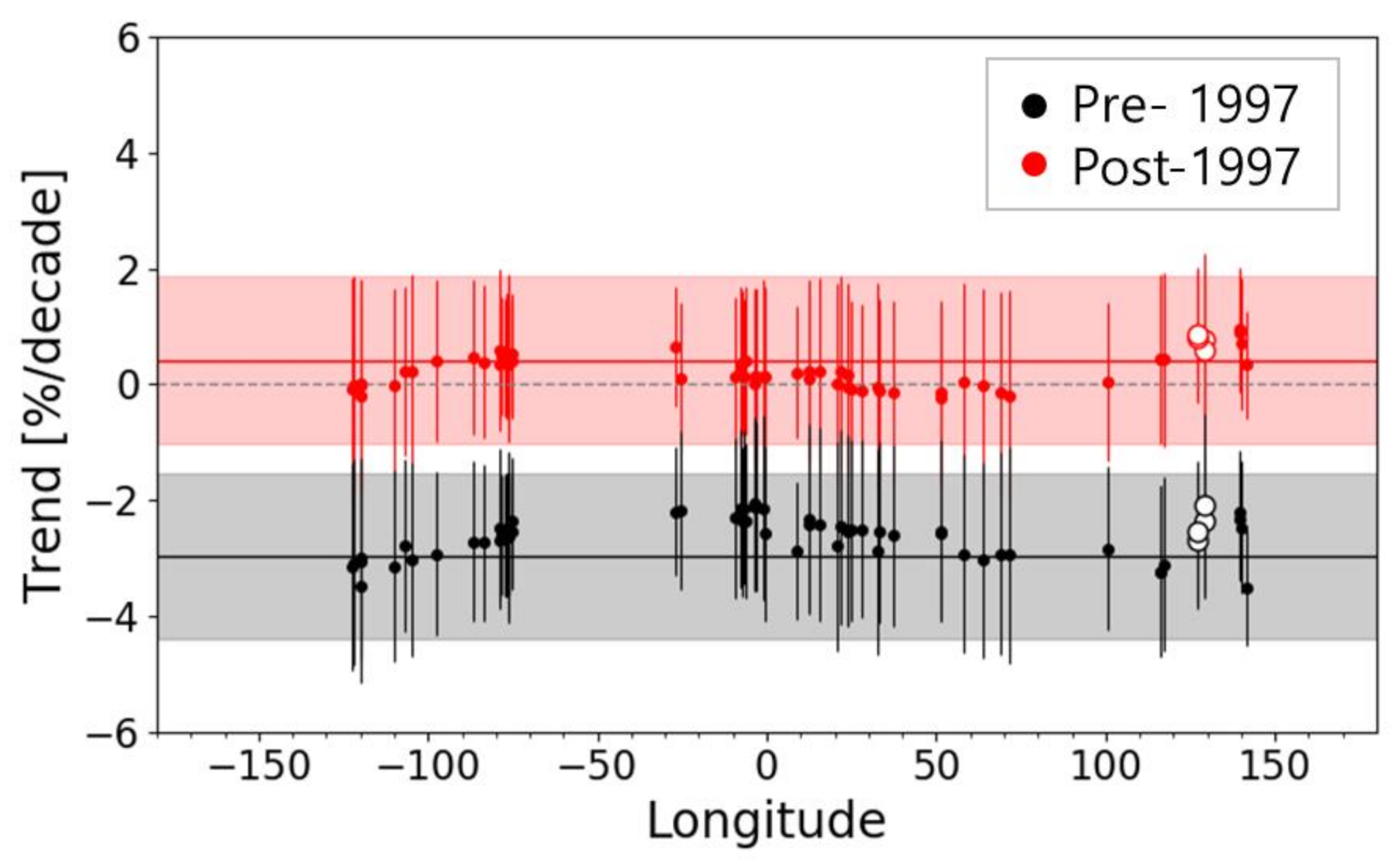
3.1. Characteristics of Ozone Trends in East Asia

The East Asia region, located in the mid-latitudes from 20–40° N, has been experiencing extreme environmental changes owing to rapid industrialization. In particular, unexpected changes in CFC emissions have recently been reported in China; therefore, a thorough investigation is required into ozone changes in East Asia. Figure 1 shows the time-series of the total column ozone and the fitted results for the MLR from 1980 to 2013 in East Asia. The regression analysis used all of the proxies listed in Table 1 and the SBUV MOD total ozone data as the dependent variable, with linear trends described by the ILT. The linear trends are divided into pre-1997 (i.e., 1980–1996) and post-1997 (i.e., 1997–2013) periods of equal lengths of 17 years to facilitate the comparison of the variability before and after the turnaround point without the influence of the number of samples. The time-series analysis results of the three latitude band averages (i.e., 0–20, 20–40, and 40–60° N) are presented together for latitudinal comparison. The ozone trend was obtained by applying the MLR model to monthly or yearly time-series, whose results are plotted in Figure 1. In the regression analysis of monthly data, anomaly values for monthly climatology were used, whereas average values were used for the analysis of yearly data. As the monthly variability is a high-frequency fluctuation compared to the annual variability, explaining all of the fluctuations with only the natural variabilities listed in Table 1 is difficult. In addition, autocorrelation is likely to be present in the monthly time-series; therefore, the adjusted R2 value of the model is low. As the short-term fluctuations, mostly due to atmospheric variability, do not have a significant effect on the long-term ozone trend, there is usually no noticeable difference in the linear trends derived from monthly and yearly time-series; however, the short-term variability increases the uncertainty in the trend. Therefore, if the analysis period is sufficiently long, analysis using yearly data may be advantageous for deriving a long-term trend. For the 20–40° N region, to which East Asia belongs, the amplitude of the time-series was larger than that of other regions; therefore, the adjusted R2 value of the model was lower. There are other causes of the variation that cannot be explained by natural variability, or high-frequency variability plays a critical role in this region. If the regression model does not fully account for the variability in the time-series, other factors not considered in the model can also affect the long-term trend, such that the uncertainty in the trend estimate increases.
The Korean Peninsula in northeastern East Asia is affected by westerly winds. As it is located on the east coast of the continent, it is greatly influenced by pollutants from China, as well as from domestic sources [49,50,51,52]. Furthermore, the Korean Peninsula is affected by seasonal monsoons owing to its geographical characteristics, i.e., located at the boundary between the ocean and continent; at the same time, the seasonal weather variation is large because it is at the boundary region between the temperate and polar climate zones. Figure 2 shows a comparison of the total column ozone trends at SBUV overpass stations in the 35–40° N range (the latitude of the Korean Peninsula), along with the trends in the band-averaged total column ozone over 35–40° N. The trends depicted in Figure 2 are two ILT divided into the pre- and post-1997 datasets, from 1980 to 2013. The error range corresponds to a 2-sigma uncertainty for the trend. The overpass stations, located between 100° E and 150° E, which spans China, the Korean Peninsula, and Japan, showed a smaller decreasing trend than the average zonal mean pre-1997 and a larger increasing trend post-1997. In particular, the stations on the Korean Peninsula (i.e., Seoul, Suwon, Pohang, and Busan), denoted by unfilled circles, exhibited these features more clearly, with a small trend uncertainty.
In general, the trend uncertainty decreased with an extension of the analysis period. Nevertheless, when the analysis period included a critical turning point in the trend, such as 1997, the uncertainty in each trend obtained by applying the ILT may be greater than when separately analyzing the two periods. Table 2 compares the trends and uncertainties in the MLR results according to the analysis period and time interval of the data. The analysis period was divided into the pre- and post-1997 periods, from 1980 to 2013; the time-series data of the total column ozone used SBUV MOD averaged over 35–40° N. For the MLR results for the entire period, the adjusted R2 value for the yearly time-series was 0.574, which was lower than the time-series averaged from 20–40° N shown in Figure 1 owing to a reduction in the spatial scale. The MLR model, which analyzed only the pre-1997 period, by reducing the period length compared with that in the previous experiment, had an adjusted R-squared value of 0.954, and proxies well explained the ozone variability, whereas the MLR model for the post-1997 period showed a sharp decline in the explanatory power of the proxies, with an adjusted R-squared value of 0.419. When the same experiments were performed on monthly data, the explanatory power of the model was lower than that of the analysis with the yearly data, but the difference in the adjusted R2 value between the pre-and post-1997 periods was significantly reduced. When comparing the trends in each experiment, the trends in the experiments for the same period were similar; however, among them, the experiments that analyzed the yearly time-series by separating the periods (i.e., MLR_pre_year and MLR_post_year) had a significantly low trend uncertainty. In particular, when the MLR analysis was carried out by separating the periods in the pre-1997 period, the trend uncertainty was more than twice as large for the monthly time-series (MLR_pre_mon) than in the experiment for the yearly time-series (MLR_pre_year). Nonetheless, in the post-1997 period, the experiments using monthly (MLR_post_mon) and yearly time-series (MLR_post_year) did not have significant differences in the trend uncertainty. Consequently, this demonstrates that there is a significant difference in the total column ozone variability before and after 1997. Therefore, conducting independent MLR analyses may be better to properly understand ozone variability in the post-1997 period.
Figure 3 shows the model contribution of the natural proxies when the analysis was performed independently for pre- and post-1997 using SBUV MOD averaged over 35–40° N, which illustrates the regression coefficient and uncertainty as the amount that contributes to ozone change (i.e., %/decade). For example, the bar for the trend proxy indicates the ozone change rate per decade based on the mean value of the analysis period. In other words, the larger the coefficient of each proxy and the smaller the uncertainty, the more significant the effect of the proxy on ozone variability. For the pre-1997 period, which was analyzed via yearly time-series, most proxies had a relatively large regression coefficient compared with the uncertainty, whereas in the post-1997 period, their coefficients were significantly reduced, and the uncertainty increased (Figure 3a) despite the sample length being the same. Otherwise, for the analysis with the monthly time-series data, the regression coefficients for the proxies in the pre- and post-1997 periods were maintained at a similar level compared to the yearly time-series analysis, but the uncertainty in the trend proxy slightly increased (Figure 3b). That is, during the pre-1997 period, the natural proxies had sufficient explanatory power with respect to the yearly ozone variability; the uncertainty in the trend estimates was low, such that the yearly time-series analysis was effective for the trend estimates. However, for the post-1997 period, it is difficult to conclude that the yearly time-series analysis is absolutely better than the monthly analysis, as the regression coefficients of the natural proxies were substantially reduced when analyzed with the yearly time-series data. These characteristics of the post-1997 period are presumed to be due to the more accelerated climate change resulting from increased GHG concentrations, along with the decline in ODS and other unknown causes, thus complicating ozone variability. In addition, a weakened phase of solar activity may have also contributed to the weakening of the effects of natural variability on ozone [53]. Accordingly, additional measures are needed to effectively derive the ozone trend in the post-1997 period. Further, the monthly time-series analysis, in which the contribution of proxies such as ENSO and AO becomes significant in the post-1997 period, may be one means to achieve this. In the next section, experimental results for the East Asia region from monthly time-series analysis and the use of atmospheric proxies are presented.

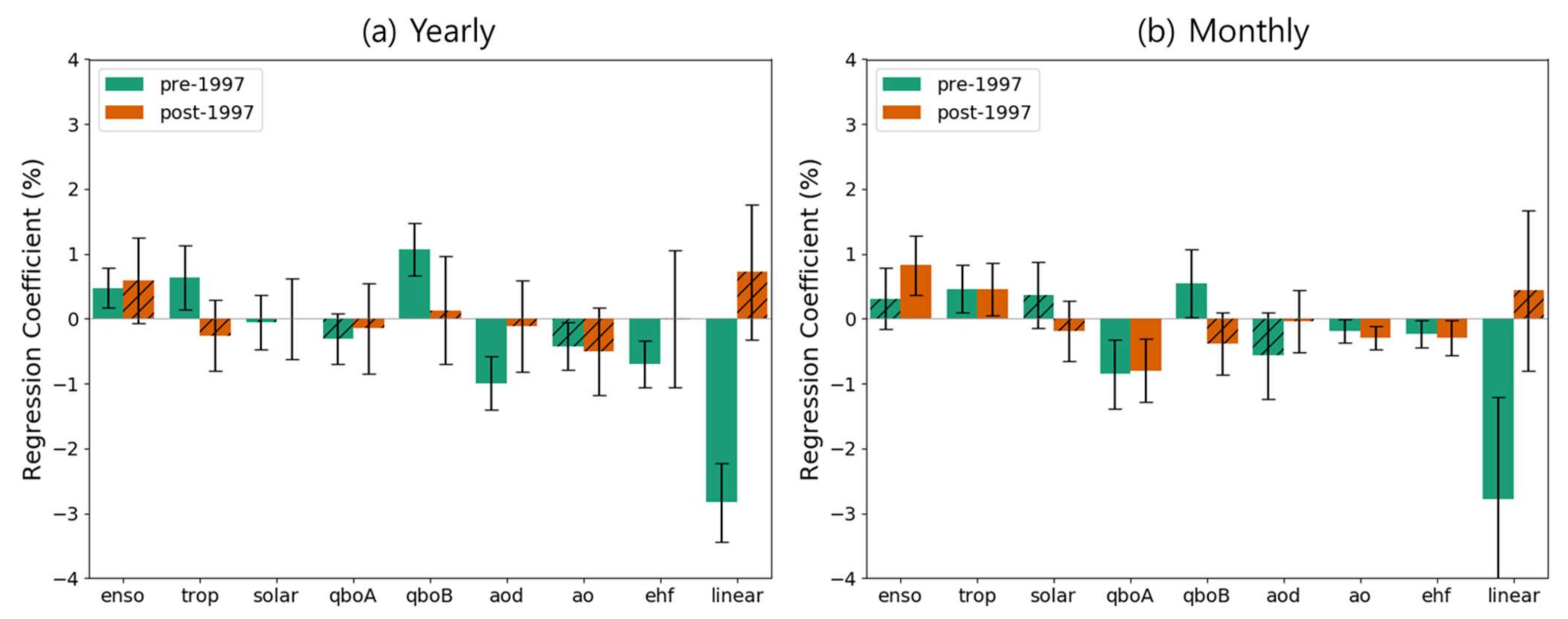
3.2. Atmospheric Proxies

As East Asia is a region with large ozone fluctuations and a large trend uncertainty, it is difficult to explain the ozone variability in this region only with natural proxies. Short-term ozone variability is more dominated by synoptic weather than natural proxies [7,43,54]. Although atmospheric variability usually does not play a significant role in long-term trends, caution should be exercised when employing it as a proxy for the total column ozone variability because it can be the result of many processes involved in complex ozone-climate feedback [7]. Nevertheless, if the analysis period is not sufficiently long or the spatial scale of the ozone variability is small, the uncertainty in the MLR model will increase, which also affects the uncertainty in the trend estimates; therefore, to mitigate this, it is necessary to consider atmospheric proxies [43,55]. Figure 4 shows a comparison of the fitted results according to the additional use of atmospheric proxies for the time-series of the total column ozone averaged over 35–40° N using the SBUV MOD. The meteorological variables used as proxies were temperature (T), geopotential height (GPH), v-component wind (V-Wind), potential vorticity (PV) related to the dynamic process affecting the ozone distribution, and time-series data for the variables obtained from ERA-5 reanalysis data. The time-series of each variable was selected as the one with the highest correlation with the total column ozone variation among altitudes of 10, 50, 100, 150, 200, 300, 500, and 850 hPa. All atmospheric proxies were used after removing seasonality by subtracting the monthly climatology. As the atmospheric proxies were added, the adjusted R2 value increased significantly for both the monthly and yearly time-series, and the trend uncertainty decreased, whereas the trend estimate did not display a significant difference.
Similarly, Figure 5 presents the fitted results according to the additional use of atmospheric proxies during the same period but using the time-series of the ozone from the merged TOMS/OMI/OMPS dataset passing over Pohang. As the spatial scale of the ozone data decreases, the amplitude of the time-series increases, and fluctuations appear at higher frequencies. Therefore, in the annual time-series analysis without atmospheric proxies, a negative adjusted R2 value indicates that the model was not fitted properly. When the atmospheric proxies were included in the annual time-series analysis, the adjusted R2 value was abnormally high owing to the high autocorrelation coefficient, and the reliability of the trend estimate was poor (Figure 5b). Moreover, neither trend estimate obtained from annual time-series analysis is considered reasonable because they both have significantly high uncertainties of 2.58 and 3.76%/decade, respectively. In contrast, in the trend analyzed by the monthly time-series (Figure 5a), the adjusted R2 value increased significantly, and the trend uncertainty decreased according to the inclusion of the atmospheric proxies. Compared with the previous ozone time-series averaged over 35–40° N, the increase in the R2 value was larger, and the decrease in the trend uncertainty was nearly identical. In conclusion, for the total column ozone variability at a small spatial scale, such as point observed data, the trend uncertainty in the annual time-series can be significant until sufficient data are obtained; in this case, the use of atmospheric proxies may further reduce the reliability of the trend. In the monthly time-series analysis, the inclusion of atmospheric proxies in the MLR analysis allowed the trend to be estimated much more effectively.
Figure 6 shows the post-1997 trends according to the analysis period and data for the MLR. In all of the analyses, the starting year of the MLR was the same (i.e., 1997) and the changes in the trend and 2-sigma uncertainty are presented with different ending years for the MLR. The panels on the left (Figure 6a,c) are the results from the SBUV MOD averaged 35–40° N data, as shown in Figure 4, whereas those on the right are from the TOMS/OMI/OMPS dataset over Pohang, as shown in Figure 5. The upper and lower panels were classified according to the use of atmospheric proxies, with the upper panels using atmospheric proxies, while the lower panels were not. When including the atmospheric proxies, the SBUV MOD time-series data, which have a relatively larger spatial scale, converge to a level similar to that of the monthly analysis within 16 years (i.e., in 2013) in the annual analysis (Figure 6a). In contrast, under the same conditions, the TOMS/OMI/OMPS time-series data over Pohang reached a stable level after at least 20 years (i.e., in 2017) (Figure 6b). A longer period of data is needed to obtain sufficient reliability. As the MLR analysis using monthly data employs a larger number of samples than the yearly data, it showed a slightly stable trend under all of the conditions shown in Figure 6, but the uncertainty was further reduced as the analysis period increased. Meanwhile, when the atmospheric proxies were not involved, the period required to converge on the trend of the annual time-series was significantly reduced; this tendency was particularly evident in the TOMS/OMI/OMPS dataset over an observed data point such as at Pohang. Conversely, in the monthly time-series analysis, the uncertainty was smaller when the atmospheric proxies were used together. In other words, the minimum analysis period required for the trend estimate to stably converge depended on the variability in data; the larger the fluctuations over short periods, such as those found in point observed data, the longer the analysis period required.

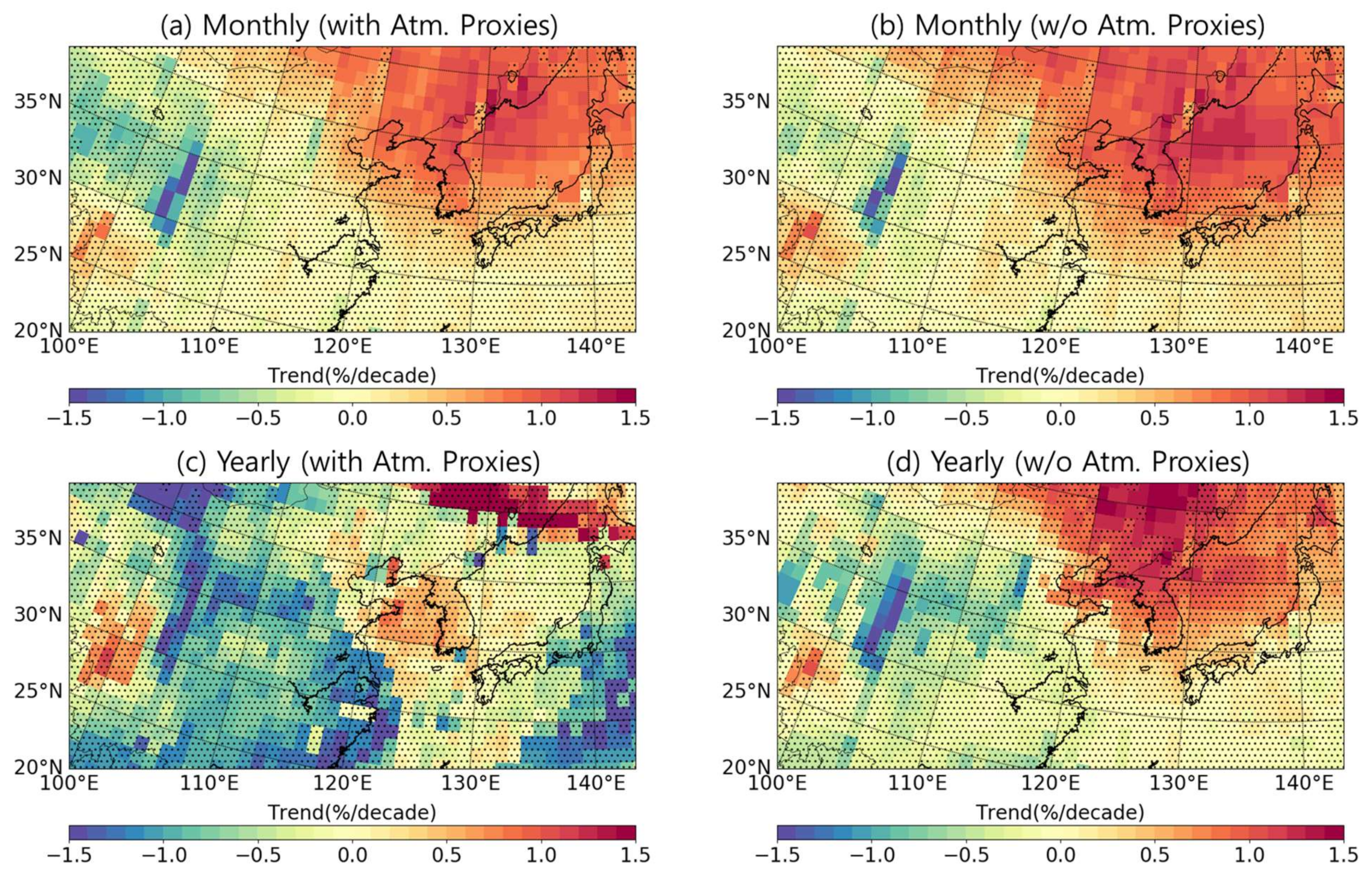
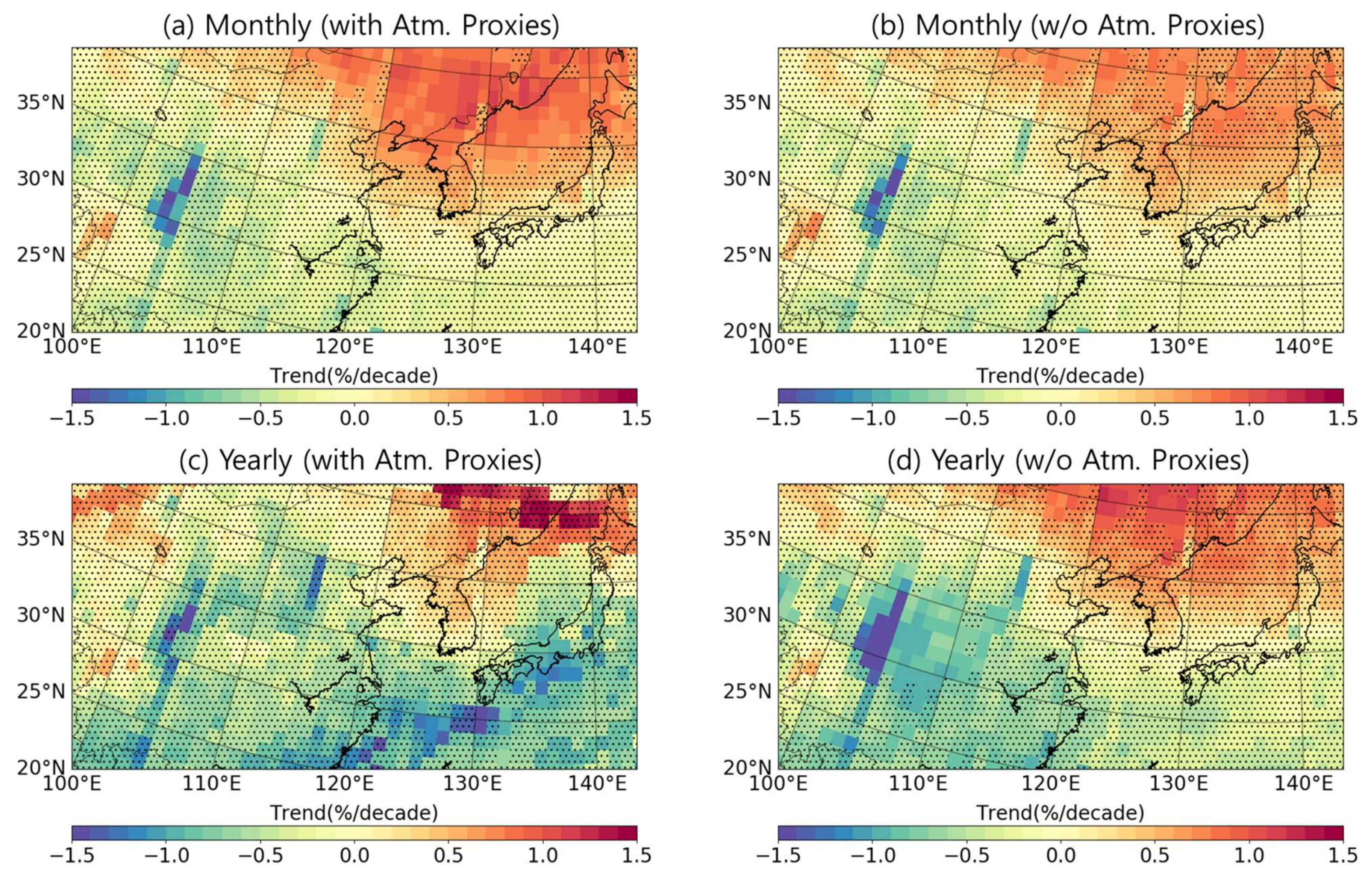
3.3. Recent Trend in East Asia

As mentioned in Section 3.1, the ozone trend reached a turning point in 1997 and has since shown a different pattern. Figure 7 shows the trend distribution of the total column ozone by region in East Asia from 1997–2017 using the TOMS/OMI/OMPS dataset. The dotted area in the figure corresponds to the region where there was no significant trend with a 95% confidence. Based on the results of the monthly time-series analysis, when the atmospheric proxies were considered, the Korean Peninsula and Manchuria regions showed a statistically significant increase of approximately 1%/decade during this period; the increasing trend in the Korean Peninsula was significantly higher than that of the surrounding latitudes. In the Korean Peninsula region, the stratosphere–troposphere exchange has recently been active; as a result, the occurrence of secondary ozone peaks has increased [16,28], and these characteristics appear to have contributed to the increasing trend in this region. In contrast, most of China showed a change of <±0.5%/decade, and the mountain range west of Chengdu showed a decrease of <–1%/decade. The decreasing trend in the mountain range west of Chengdu is common in all of the analyses shown in Figure 7. According to a previous study, the recovery of the ozone on the Tibetan Plateau is lower than the average for that latitude [56]. The exaggerated decreasing trend is presumed to originate from the complexity of the climatic and environmental characteristics of the region, located on the border between the Tibetan Plateau and the metropolitan area of western China, which may have contributed to the noticeable decreasing trend. When the trend was estimated from the monthly time-series without atmospheric proxies, the trend distribution was similar to the case of using the atmospheric proxies, but the overall increase was slightly higher. In other words, the atmospheric proxy variables contributed to the increase in the total column ozone (a part of the increase in the ozone can be explained by the atmospheric proxy variables, weakening the linear trend), but the quantitative contribution was not large (approximately 0.15%/decade). Meanwhile, the trend estimated from the yearly variability in the ozone showed a pattern similar to that of the monthly variability. However, as shown in Figure 5, the uncertainty in the trend increased owing to an insufficient analysis period; thus, the region with a statistically insignificant trend expanded with the growth of regional deviation. If the atmospheric proxies are additionally considered here, these characteristics become even larger, and the statistically significant trend almost disappears in this region.
Owing to technical limitations, satellite data actually provide ozone values averaged over a range of approximately several to tens of kilometers, whereas ground observation data observe the variability in ozone at specific points. Figure 8 compares the increasing trend of the Korean Peninsula in the analysis of the TOMS/OMI/OMPS dataset with the Brewer ground observation data observed in Pohang and Seoul. Considering that these are highly variable point observation data, they were analyzed as monthly time-series data, and both natural and atmospheric proxies were used. Although some missing data exist in both ground observation datasets, they show similar variations owing to their relatively close distance. In addition, as in the satellite composite dataset, a slightly higher rate of increase was observed in Seoul, which is located inland at high latitudes, than in Pohang, which is located on the eastern coast of the Korean Peninsula. The ground observation data exhibit a larger increasing trend and uncertainty than the trend obtained from the TOMS/OMI/OMPS dataset, and the difference between the stations is also larger. Based on the variability by station, the fluctuation in the ground observation data at Pohang is particularly large; therefore, there is no statistically significant increase. Subsequently, the long-term variations in the total column ozone observed on the ground show high-frequency fluctuations owing to the smaller spatial scale compared to the TOMS/OMI/OMPS dataset, but the regional distribution of the trend is mostly consistent with the satellite-merged dataset.
While ozone observation at Pohang was terminated in 2017, the satellite-merged dataset continued to accumulate data. To examine the characteristics of recent ozone variability, the trend in East Asia until 2020 is shown in Figure 9 using the satellite-merged dataset. When the period is extended, all of the trends according to the time interval of the time-series or the inclusion of atmospheric proxies converge. Comparing the overall change from the previous period, the increasing trend in the Korean Peninsula and Manchuria decreased. In particular, the regions that showed statistically significant increases in the monthly analyzed trend without atmospheric proxies (Figure 9b) did not show a statistically significant trend. Contrary to the previous period from 1997 to 2017, when atmospheric proxies were considered, the overall increasing trend was higher, and this difference was even greater in the Korean Peninsula and Manchuria regions. In other words, from 1997 to 2020, the atmospheric proxies contributed to the reduction in the total column ozone, and the trend difference depending on the atmospheric proxies was approximately 0.26%/decade, which was larger than that from 1997 to 2017. Additionally, in the monthly analyzed trend that did not include the atmospheric proxies in the Korean Peninsula and Manchuria, the large difference between the 1997–2017 and 1997–2020 periods indicates that the influence of atmospheric variability on the total column ozone has been recently increasing. Figure 10 illustrates the contribution of the atmospheric proxies to the ozone anomaly in the TOMS/OMI/OMPS dataset over Pohang. If we focus on recent years, the contribution of atmospheric proxies has been biased in a relatively negative direction since approximately 2016. When the total contribution of the atmospheric proxies was averaged for each period before and after 2017, the contribution amount was +0.03%/decade before 2017 and –0.17%/decade after 2017, showing that the contribution to ozone reduction has recently increased. According to the WMO 2015–2019 Global Climate Report [57], the last five years (2015–2019) have witnessed the warmest temperatures on record globally, and the atmospheric concentration of CO2 has increased by 18% or more compared to the previous five years, indicating that global warming is accelerating. Such climatic characteristics have also affected changes in the ozone concentration; therefore, it is necessary to continuously monitor whether these changes continue in the future.

4. Conclusions

The change in the total column ozone in East Asia has shown a greater range of fluctuation and greater uncertainty than other regions. Within the variability in the total column ozone in East Asia after 1997, the uncertainty in the trend expanded with a decrease in the contribution of natural components. The use of monthly time-series data and atmospheric proxies can be a means of reducing trend uncertainty in East Asia during the post-1997 period. In general, if the sample size is sufficiently large, there is no significant difference between the trends derived from the monthly and annual time-series analyses. For time-series data of the total ozone averaged over several degreewide latitude bands, annual time-series analysis provided a trend with lower uncertainty than monthly time-series analysis. However, it is necessary to examine whether the analysis provides a reasonable trend when the analysis period is short or when the spatial scale of the data is small, as the analysis of annual variability can accomodate considerable uncertainty owing to overfitting. Furthermore, as atmospheric proxies have a mutual influence on changes in the ozone, some characteristics may differ from those that do not include atmospheric proxies in that the atmospheric proxies partly involve the ozone-climate feedback effect. Nevertheless, atmospheric proxies can play a significant role in the trend analysis of the monthly time-series since 1997 when the trend uncertainty is large, as atmospheric proxies significantly reduce the uncertainty in the monthly ozone variability. Consequently, in the recent trend analysis for total ozone over East Asia, monthly MLR analysis using additional atmospheric proxies provides the most reliable trends.
The trend distribution of the total column ozone from 1997 to 2017 in East Asia showed a large increase of approximately 1%/decade in the Korean Peninsula and Manchuria, whereas this was <0.5%/decade in most of China. Based on the analysis of ground observation data from Pohang and Seoul using a Brewer ozone spectrophotometer, a similar tendency was confirmed, although the range of the fluctuation and trend uncertainty was higher. When the analysis period was extended to 2020, the increase across the Korean Peninsula and Manchuria regions slightly decreased, and the contribution of atmospheric proxies to changes in the ozone increased. Based on this study, we confirmed that the trend in the total column ozone in East Asia since 1997 was affected by both ODS reduction in the atmosphere and recent climate change. In particular, the climatic and environmental importance and peculiarity of the East Asian region signify the need for continuous monitoring and multi-faceted analysis of this region. In addition, to fundamentally understand ozone variability, it is necessary to closely analyze the characteristics of these changes according to the altitude and the contribution of influencing factors.

Author Contributions

Conceptualization, D.S. and Y.-S.O.; writing—original draft preparation, D.S.; writing—review and editing, Y.-S.O. and C.-Y.C.; resources, W.S. and J.-H.K.; data curation, W.S. All authors have read and agreed to the published version of the manuscript.

Funding

This study was funded by the Korea Meteorological Administration Research and Development Program “Development of Monitoring and Analysis Techniques for Atmospheric Composition in Korea” under Grant (KMA2018-00522).

Data Availability Statement

Data describing the natural variability are listed in Table 1. The ground observation data are available on request from the National Institute of Meteorological Sciences (Daegeun Shin, [email protected]) for the Pohang Brewer data and Yeonsei University (Ja-Ho Koo, [email protected]) for the Seoul Brewer data. The SBUV MOD dataset is available at https://acd-ext.gsfc.nasa.gov/Data_services/merged/, accessed on 5 January 2021. TOMS, OMI, and OMPS data are available at https://search.earthdata.nasa.gov/search/, accessed on 12 December 2020. ERA5 reanalysis data are available at https://www.ecmwf.int/en/forecasts/datasets/reanalysis-datasets/era5/, accessed on 24 February 2021.

Acknowledgments

The total column ozone data from Seoul were provided by the Atmospheric Radiation Laboratory at Yeonsei University. We would like to acknowledge all of the researchers, including Ja-Ho Koo, Joon Kim and Hi Ku Cho, for their efforts to produce high-quality data.

Conflicts of Interest

The authors declare no conflict of interest.

References

  1. Ko, M.K.W.; Newman, P.A.; Reimann, S. ; Lifetimes of Stratospheric Ozone-Depleting Substances, Their Replacements, and Related Species, World Climate Research Programme; SPARC: Devens, MA, USA, 2013; Avaliable online: https://www.sparc-climate.org/fileadmin/customer/6_Publications/SPARC_reports_PDF/6_SPARC_LifetimeReport_Web.pdf (accessed on 28 July 2021).
  2. World Meteorological Organization (WMO). Scientific Assessment of Ozone Depletion: 2018, Global Ozone Research and Monitoring Project—Report No. 58; World Meteorological Organization (WMO): Geneva, Switzerland, 2018. [Google Scholar]
  3. SPARC/IO3C/GAW Report on Long-term Ozone Trends and Uncertainties in the Stratosphere; SPARC: Devens, MA, USA, 2019; Available online: www.sparc-climate.org/publications/sparc-reports (accessed on 28 July 2021).
  4. Weber, M.; Coldewey-Egbers, M.; Fioletov, V.E.; Frith, S.M.; Wild, J.D.; Burrows, J.P.; Long, C.S.; Loyola, D. Total ozone trends from 1979 to 2016 derived from five merged observational datasets—The emergence into ozone recovery. Atmos. Chem. Phys. 2018, 18, 2097–2117. [Google Scholar] [CrossRef] [Green Version]
  5. Zerefos, C.; Kapsomenakis, J.; Eleftheratos, K.; Tourpali, K.; Petropavlovskikh, I.; Hubert, D.; Godin-Beekmann, S.; Steinbrecht, W.; Frith, S.; Sofieva, V.; et al. Representativeness of single lidar stations for zonally averaged ozone profiles, their trends and attribution to proxies. Atmos. Chem. Phys. 2018, 18, 6427–6440. [Google Scholar] [CrossRef] [Green Version]
  6. Dyominov, I.G.; Zadorozhny, A.M. Greenhouse gases and recovery of the Earth’s ozone layer. Adv. Space Res. 2005, 35, 1369–1374. [Google Scholar] [CrossRef]
  7. Chipperfield, M.; Bekki, S.; Dhomse, S.; Harris, N.; Hassler, B.; Hossaini, R.; Steinbrecht, W.; Thieblemont, R.; Weber, M. Detecting recovery of the stratospheric ozone layer. Nature 2017, 549, 211–218. [Google Scholar] [CrossRef] [PubMed] [Green Version]
  8. Banerjee, A.; Maycock, A.C.; Archibald, A.T.; Abraham, N.L.; Telford, P.; Braesicke, P.; Pyle, J.A. Drivers of changes in stratospheric and tropospheric ozone between year 2000 and 2100. Atmos. Chem. Phys. 2016, 16, 2727–2746. [Google Scholar] [CrossRef] [Green Version]
  9. Molina, M.; Rowland, F. Stratospheric sink for chlorofluoromethanes: Chlorine atom-catalysed destruction of ozone. Nature 1974, 249, 810–812. [Google Scholar] [CrossRef]
  10. Stolarski, R.S.; Cicerone, R.J. Stratospheric chlorine: A possible sink for ozone. Can. J. Chem. 1974, 52, 1610–1615. [Google Scholar] [CrossRef]
  11. Haigh, J.D.; Pyle, J.A. Ozone perturbation experiments in a two-dimensional circulation model. Q. J. R. Meteorol. Soc. 1982, 108, 551–574. [Google Scholar] [CrossRef]
  12. Jonsson, A.I.; Fomichev, V.I.; Shepherd, T.G. The effect of nonlinearity in CO2 heating rates on the attribution of stratospheric ozone and temperature changes. Atmos. Chem. Phys. 2009, 9, 8447–8452. [Google Scholar] [CrossRef] [Green Version]
  13. Collins, W.J.; Derwent, R.G.; Garnier, B.; Johnson, C.E.; Sanderson, M.G. Effect of stratosphere-troposphere exchange on the future tropospheric ozone trend. J. Geophys. Res. 2003, 108. [Google Scholar] [CrossRef] [Green Version]
  14. Hwang, S.-H.; Kim, J.; Cho, G.-R. Observation of secondary ozone peaks near the tropopause over the Korean peninsula associated with stratosphere-troposphere exchange. J. Geophys. Res. 2007, 112. [Google Scholar] [CrossRef] [Green Version]
  15. Hegglin, M.; Shepherd, T. Large climate-induced changes in ultraviolet index and stratosphere-to-troposphere ozone flux. Nat. Geosci. 2009, 2, 687–691. [Google Scholar] [CrossRef]
  16. Park, S.S.; Kim, J.; Cho, H.K.; Lee, H.; Lee, Y.; Miyagawa, K. Sudden increase in the total ozone density due to secondary ozone peaks and its effect on total ozone trends over Korea. Atmos. Environ. 2012, 47, 226–235. [Google Scholar] [CrossRef]
  17. Newman, P.A.; Daniel, J.S.; Waugh, D.W.; Nash, E.R. A new formulation of equivalent effective stratospheric chlorine (EESC). Atmos. Chem. Phys. 2007, 7, 4537–4552. [Google Scholar] [CrossRef] [Green Version]
  18. Randel, W.J.; Wu, F.A. Stratospheric ozone profile data set for 1979–2005: Variability, trends, and comparisons with column ozone data. J. Geophys. Res. Atmos. 2007, 112, D06313. [Google Scholar] [CrossRef] [Green Version]
  19. World Meteorological Organization (WMO). Scientific Assessment of Ozone Depletion: 2014, Global Ozone Research and Monitoring Project—Report No. 55; World Meteorological Organization (WMO): Geneva, Switzerland, 2014. [Google Scholar]
  20. Dhomse, S.S.; Kinnison, D.; Chipperfield, M.P.; Salawitch, R.; Cionni, I.; Hegglin, M.I.; Abraham, N.L.; Akiyoshi, H.; Archibald, A.T.; Bednarz, E.M.; et al. Estimates of ozone return dates from Chemistry—Climate Model Initiative simulations. Atmos. Chem. Phys. Discuss. 2018, 18, 8409–8438. [Google Scholar] [CrossRef] [Green Version]
  21. Butchart, N. The Brewer-Dobson circulation. Revs. Geophys. 2014, 52, 157–184. [Google Scholar] [CrossRef]
  22. Flury, T.; Wu, D.L.; Read, W.G. Variability in the speed of the Brewer–Dobson circulation as observed by Aura/MLS. Atmos. Chem. Phys. 2013, 13, 4563–4575. [Google Scholar] [CrossRef] [Green Version]
  23. Rigby, M.; Park, S.; Saito, T.; Western, L.M.; Redington, A.L.; Fang, X.; Henne, S.; Manning, A.J.; Prinn, R.G.; Dutton, G.S.; et al. Increase in CFC-11 emissions from eastern China based on atmospheric observations. Nature 2019, 569, 546–550. [Google Scholar] [CrossRef] [PubMed]
  24. Dhomse, S.S.; Feng, W.; Montzka, S.A.; Hossaini, R.; Keeble, J.; Pyle, J.A.; Daniel, J.S.; Chipperfield, M.P. Delay in recovery of the Antarctic ozone hole from unexpected CFC-11 emissions. Nat. Commun. 2019, 10, 5781. [Google Scholar] [CrossRef] [PubMed] [Green Version]
  25. Montzka, S.A.; Dutton, G.S.; Yu, P.; Ray, E.; Portmann, R.W.; Daniel, J.S.; Kuijpers, D.L.; Hall, B.D.; Mondeel, D.; Siso, C.; et al. An unexpected and persistent increase in global emissions of ozone-depleting CFC. Nature 2018, 557, 413–417. [Google Scholar] [CrossRef] [PubMed]
  26. Kim, J.; Jeong, U.; Ahn, M.; Kim, J.H.; Park, R.J.; Lee, H.; Song, C.H.; Choi, Y.; Lee, K.; Yoo, J.; et al. New Era of Air Quality Monitoring from Space: Geostationary Environment Monitoring Spectrometer (GEMS). Bull. Am. Meteorol. Soc. 2020, 101, E1–E22. [Google Scholar] [CrossRef] [Green Version]
  27. Kim, J.; Cho, H.K.; Lee, Y.G.; Oh, S.N.; Baek, S.-K. Updated trends of stratospheric ozone over Seoul. J. Atmos. 2005, 15, 101–118. [Google Scholar]
  28. Shin, D.; Song, S.; Ryoo, S.-B.; Lee, S.-S. Variations in Ozone Concentration over the Mid-Latitude Region Revealed by Ozonesonde Observations in Pohang, South Korea. Atmosphere 2020, 11, 746. [Google Scholar] [CrossRef]
  29. McPeters, R.D.; Bhartia, P.K.; Haffner, D.; Labow, G.J.; Flynn, L. The version 8.6 SBUV ozone data record: An overview. J. Geophys. Res. Atmos. 2013, 118, 8032–8039. [Google Scholar] [CrossRef] [Green Version]
  30. Frith, S.M.; Kramarova, N.A.; Stolarski, R.S.; McPeters, R.D.; Bhartia, P.K.; Labow, G.J. Recent changes in total column ozone based on the SBUV Version 8.6 Merged Ozone Data Set. J. Geophys. Res. Atmos. 2014, 119, 9735–9751. [Google Scholar] [CrossRef]
  31. DeLand, M.T.; Taylor, S.L.; Huang, L.K.; Fisher, B.L. Calibration of the SBUV version 8.6 ozone data product. Atmos. Meas. Tech. 2012, 5, 2951–2967. [Google Scholar] [CrossRef] [Green Version]
  32. Bhartia, P.K.; McPeters, R.D.; Flynn, L.E.; Taylor, S.; Kramarova, N.A.; Frith, S.; Fisher, B.; DeLand, M. Solar Backscatter UV (SBUV) total ozone and profile algorithm. Atmos. Meas. Tech. 2013, 6, 2533–2548. [Google Scholar] [CrossRef] [Green Version]
  33. Kramarova, N.A.; Bhartia, P.; Frith, S.M.; McPeters, R.D.; Stolarski, R.S. Interpreting SBUV smoothing errors: An example using the quasi-biennial oscillation. Atmospheric Meas. Tech. 2013, 6, 2089–2099. [Google Scholar] [CrossRef] [Green Version]
  34. Kramarova, N.A.; Frith, S.M.; Bhartia, P.; McPeters, R.D.; Taylor, S.L.; Fisher, B.L.; Labow, G.J.; Deland, M.T. Validation of ozone monthly zonal mean profiles obtained from the version 8.6 Solar Backscatter Ultraviolet algorithm. Atmos. Chem. Phys. 2013, 13, 6887–6905. [Google Scholar] [CrossRef] [Green Version]
  35. TOMS Science Team (Unrealeased). TOMS Earth Probe Total Column Ozone Daily L3 Global 1 deg × 1.25 deg Lat/Lon Grid V008; Goddard Earth Sciences Data and Information Services Center (GES DISC): Greenbelt, MD, USA, 2005; Volume 15, pp. 101–118. Available online: https://disc.gsfc.nasa.gov/datacollection/TOMSEPL3dtoz_008.html (accessed on 12 December 2020).
  36. Bhartia, P.K. OMI/Aura TOMS-Like Ozone, Aerosol Index, Cloud Radiance Fraction L3 1 Day 1 Degree × 1 Degree V3; NASA Goddard Space Flight Center, Goddard Earth Sciences Data and Information Services Center (GES DISC): Greenbelt, MD, USA, 2012. [Google Scholar] [CrossRef]
  37. Jaross, G. OMPS-NPP L3 NM Ozone (O3) Total Column 1.0 Deg Grid Daily V2; Goddard Earth Sciences Data and Information Services Center (GES DISC): Greenbelt, MD, USA, 2017. [Google Scholar] [CrossRef]
  38. Chehade, W.; Weber, M.; Burrows, J.P. Total ozone trends and variability during 1979–2012 from merged datasets of various satellites. Atmos. Chem. Phys. 2014, 14, 7059–7074. [Google Scholar] [CrossRef] [Green Version]
  39. Steinbrecht, W.; Froidevaux, L.; Fuller, R.; Wang, R.; Anderson, J.; Roth, C.; Bourassa, A.; Degenstein, D.; Damadeo, R.; Zawodny, J.; et al. An update on ozone profile trends for the period 2000 to 2016. Atmos. Chem. Phys. 2017, 17, 10675–10690. [Google Scholar] [CrossRef] [Green Version]
  40. Staehelin, J.; Harris, N.R.P.; Appenzeller, C.; Eberhard, J. Ozone trends: A review. Revs. Geophys. 2001, 39, 231–290. [Google Scholar] [CrossRef] [Green Version]
  41. Dhomse, S.; Weber, M.; Wohltmann, I.; Rex, M.; Burrows, J.P. On the possible causes of recent increases in northern hemispheric total ozone from a statistical analysis of satellite data from 1979 to 2003. Atmos. Chem. Phys. 2006, 6, 1165–1180. [Google Scholar] [CrossRef] [Green Version]
  42. Poulain, V.; Bekki, S.; Marchand, M.; Chipperfield, M.P.; Khodri, M.; Lefèvre, F.; Dhomse, S.; Bodeker, G.E.; Toumi, R.; De Maziere, M.; et al. Evaluation of the inter-annual variability of stratospheric chemical composition in chemistry-climate models using ground-based multi species time series. J. Atmos. Sol. Terr. Phys. 2016, 145, 61–84. [Google Scholar] [CrossRef] [Green Version]
  43. Ziemke, J.R.; Chandra, S.; McPeters, R.D.; Newman, P.A. Dynamical proxies of column ozone with applications to global trend models. J. Geophys. Res. 1997, 102, 6117–6129. [Google Scholar] [CrossRef]
  44. Bodeker, G.; Boyd, I.S.; Matthews, W.A. Trends and variability in vertical ozone and temperature profiles measured by ozonesondes at Lauder, New Zealand: 1986–1996. J. Geophys. Res. Space Phys. 1998, 103, 28661–28681. [Google Scholar] [CrossRef]
  45. Brunner, D.; Staehelin, J.; Maeder, J.A.; Wohltmann, I.; Bodeker, G.E. Variability and trends in total and vertically resolved stratospheric ozone based on the CATO ozone data set. Atmos. Chem. Phys. 2006, 6, 4985–5008. [Google Scholar] [CrossRef] [Green Version]
  46. Harris, N.R.P.; Hassler, B.; Tummon, F.; Bodeker, G.E.; Hubert, D.; Petropavlovskikh, I.; Steinbrecht, W.; Anderson, J.; Bhartia, P.K.; Boone, C.D.; et al. Past changes in the vertical distribution of ozone–Part 3: Analysis and interpretation of trends. Atmos. Chem. Phys. 2015, 15, 9965–9982. [Google Scholar] [CrossRef] [Green Version]
  47. Kuttippurath, J.; Bodeker, G.E.; Roscoe, H.K.; Nair, P.J. A cautionary note on the use of EESC-based regression analysis for ozone trend studies. Geophys. Res. Lett. 2015, 42, 162–168. [Google Scholar] [CrossRef] [Green Version]
  48. Vyushin, D.I.; Shepherd, T.G.; Fioletov, V.E. On the statistical modeling of persistence in total ozone anomalies. J. Geophys. Res. 2010, 115, D16306. [Google Scholar] [CrossRef] [Green Version]
  49. Lee, H.J.; Jo, H.Y.; Kim, S.W.; Park, M.S.; Kim, C.H. Impacts of atmospheric vertical structures on transboundary aerosol transport from China to South Korea. Sci. Rep. 2019, 9, 13040. [Google Scholar] [CrossRef] [PubMed]
  50. Lee, S.; Kim, J.; Choi, M.; Hong, J.; Lim, H.; Eck, T.F.; Holben, B.N.; Ahn, J.-Y.; Kim, J.; Koo, J.-H. Analysis of long-range transboundary transport (LRTT) effect on Korean aerosol pollution during the KORUS-AQ campaign. Atmos. Environ. 2019, 204, 53–67. [Google Scholar] [CrossRef]
  51. Eguchi, K.; Uno, I.; Yumimoto, K.; Takemura, T.; Shimizu, A.; Sugimoto, N.; Liu, Z. Trans-pacific dust transport: Integrated analysis of NASA/CALIPSO and a global aerosol transport model. Atmos. Chem. Phys. 2009, 9, 3137–3145. [Google Scholar] [CrossRef] [Green Version]
  52. Itahashi, S.; Uno, I.; Kim, S. Seasonal source contributions of tropospheric ozone over East Asia based on CMAQeHDDM. Atmos. Environ. 2013, 70, 204–217. [Google Scholar] [CrossRef]
  53. Gaikovich, K.P.; Kropotkina, E.P.; Rozanov, S.B. Statistical Analysis of 1996–2017 Ozone Profile Data Obtained by Ground-Based Microwave Radiometry. Remote Sens. 2020, 12, 3374. [Google Scholar] [CrossRef]
  54. Braesicke, P.; Brühl, C.; Dameris, M.; Deckert, R.; Eyring, V.; Giorgetta, M.A.; Mancini, E.; Manzini, E.; Pitari, G.; Pyle, J.A.; et al. A model intercomparison analysing the link between column ozone and geopotential height anomalies in January. Atmos. Chem. Phys. 2008, 8, 2519–2535. [Google Scholar] [CrossRef] [Green Version]
  55. Krzyścin, J.W.; Degórska, M.; Rajewska-Więch, B. Impact of interannual meteorological variability on total ozone in northern middle latitudes: A statistical approach. J. Geophys. Res. 2001, 106, 17953–17960. [Google Scholar] [CrossRef] [Green Version]
  56. Li, Y.; Chipperfield, M.P.; Feng, W.; Dhomse, S.S.; Pope, R.J.; Li, F.; Guo, D. Analysis and attribution of total column ozone changes over the Tibetan Plateau during 1979. Atmos. Chem. Phys. 2020, 20, 8627–8639. [Google Scholar] [CrossRef]
  57. World Meteorological Organization (WMO). WMO Report on The Global Climate in 2015–2019; World Meteorological Organization (WMO): Geneva, Switzerland, 2019. [Google Scholar]
Figure 1. Time-series of the monthly (a,c,e) and yearly (b,d,f) SBUV total column ozone for three latitudes of 40–60° N (a,b), 20–40° N (c,d), and 0–20° N (e,f). The black and red lines represent the observed and MLR fitted ozone, respectively. Linear trends (gray dotted line) and 2σ uncertainties, as derived from the MLR, are indicated for the pre-1997 (Trend1, 1980–1996) and post–1997 (Trend2, 1997–2013) periods.
Atmosphere 12 00982 g001
Figure 2. Total column ozone trends at the SBUV overpass stations from the yearly time-series in latitudes between 35–40° N. The black and red-colored features are related trends for the pre-1997 and post-1997 datasets, respectively. Each point and error bar indicate the trends and 2-sigma uncertainty, respectively, for each SBUV overpass station; unfilled (white) points correspond to stations in the Korean Peninsula. Horizontal solid lines and the shaded range indicate the trend and 2-sigma error for the averaged total column ozone over 35–40° N.
Atmosphere 12 00982 g002
Figure 3. Normalized regression coefficients with 2-sigma error bars for each proxy from the yearly (a) and monthly (b) MLR analysis using SBUV MOD averaged over 35–40° N. The proxies with a p-value > 0.05 are presented as shaded bars.
Atmosphere 12 00982 g003
Figure 4. Time-series of SBUV zonal averaged total column ozone in latitudes between 35–40° N according to the use of atmospheric proxies. Both the monthly (a) and yearly (b) MLR fitted data are presented for comparison. The MLR fitted data without atmospheric proxies are indicated as blue lines and correspond to Trend1 and R2_adj1 while the MLR fitted data with the atmospheric proxies are indicated as red lines and correspond to Trend2 and R2_adj2.
Atmosphere 12 00982 g004
Figure 5. Time-series of TOMS/OMI/OMPS total column ozone passing over the Pohang station according to the use of atmospheric proxies. Both the monthly (a) and yearly (b) MLR fitted data are presented for comparison. The MLR fitted data without atmospheric proxies are indicated as blue lines and correspond to Trend1 and R2_adj1 while the MLR fitted data with the atmospheric proxies are indicated as red lines and correspond to Trend2 and R2_adj2.
Atmosphere 12 00982 g005
Figure 6. Dependence of analysis periods for the SBUV zonal averaged between 35–40° N (a,c) and TOMS/OMI/OMPS data over Pohang (b,d) in the MLR analysis. The start year for all analysis is fixed to 1997 and the x-axis means the end year of the analysis periods. The upper panels (a,b) use atmospheric proxies and the bottom panels (c,d) do not use atmospheric proxies. The red and black lines are the results from the yearly and monthly MLR fits, respectively. The vertical bars show the 2-sigma uncertainties in the trends.
Atmosphere 12 00982 g006
Figure 7. Trend distribution in East Asia from 1997–2017. The left panels show the trends using the atmospheric proxies (a,c), while the right panels do not (b,d). The top and bottom panels show the trends from the monthly (a,b) and yearly (c,d) variability, respectively. The dotted pattern denotes areas where trends are not statistically significant at the 2-sigma level.
Atmosphere 12 00982 g007
Figure 8. Time-series of the monthly total column ozone from the TOMS/OMI/OMPS dataset and Brewer spectrophotometer in Pohang (a) and Seoul (b). The TOMS/OMI/OMPS dataset is indicated as blue lines and corresponds to Trend1 and R2_adj1, while the Brewer observation data are indicated as black lines and correspond to Trend2 and R2_adj2. The dotted line denotes the trend derived through the MLR analysis based on each dataset.
Atmosphere 12 00982 g008
Figure 9. Trend distribution in East Asia from 1997–2020. The left panels show the trends using the atmospheric proxies (a,c), while the right panels do not (b,d). The top and bottom panels show the trends from the monthly (a,b) and yearly (c,d) variability, respectively. The dotted pattern denotes areas where trends are not statistically significant at the 2-sigma level.
Atmosphere 12 00982 g009
Figure 10. Contributions of atmospheric proxies with emphasized colors from 1997 to 2020 over Pohang from the TOMS/OMI/OMPS satellite-merged data.
Atmosphere 12 00982 g010
Table 1. Proxies and data sources used for the multi-linear regression analysis.
ProxyParameterData Sources
Solar cycle10.7 cm solar radio fluxNOAA National Centers for Environmental Information:
https://www.ngdc.noaa.gov/stp/solar/flux.html, accessed on 3 December 2020.
National Research Council Canada Dominion Radio Astrophysical Observatory:
https://spaceweather.gc.ca/forecast-prevision/solar-solaire/solarflux/sx-5-en.php, accessed on 23 October 2020.
QBOEOF1 and EOF2Free University of Berlin:
https://www.geo.fu-erlin.de/en/met/ag/strat/produkte/qbo/, accessed on 12 January 2021.
ENSOMultivariate ENSO indexNOAA Physical Sciences Laboratory:
https://psl.noaa.gov/enso/mei/, accessed on 22 March 2021.
AODMean aerosol optical depth at 550 nmNASA Goddard Institute for Space Studies:
https://data.giss.nasa.gov/modelforce/strataer/, accessed on 7 January 2021
AOArctic Oscillation (AO) indexNOAA National Weather Service Climate Prediction Center:
https://www.cpc.ncep.noaa.gov/products/precip/CWlink/daily_ao_index/ao.shtml, accessed on 16 February 2021.
Tropopause HeightTropopause pressure (TP)NOAA Physical Sciences Laboratory:
https://psl.noaa.gov/data/gridded/data.ncep.reanalysis.derived.html, accessed on 15 December 2020.
Eddy heat fluxEddy heat flux (EHF) at 100 hPaCalculated from ECMWF-ERA5 data:
https://www.ecmwf.int/en/forecasts/datasets/reanalysis-datasets/era5/, accessed on 19 January 2021.
Table 2. Trends and 2-sigma uncertainties derived from the monthly and yearly MLR analysis for the zonal averaged SBUV total column ozone between 35–40° N.
Experiment Name Time Interval of DataR2_adjTrend and Uncertainty
(%/Decade)
Linear Trend Type and Period
Pre-1997
MLR_ent_yearYearly0.574−2.97 ± 1.44ILT for the entire period
MLR_pre_yearYearly0.954−2.81 ± 0.60SLT for pre-1997
MLR_ent_monMonthly0.136−2.71 ± 1.62ILT for the entire period
MLR_pre_monMonthly0.169−2.78 ± 1.57SLT for pre-1997
Post-1997
MLR_ent_yearYearly0.5740.41 ± 1.45ILT for the entire period
MLR_post_yearYearly0.4190.72 ± 1.04SLT for post-1997
MLR_ent_monMonthly0.1360.58 ± 1.60ILT for the entire period
MLR_post_monMonthly0.1670.43 ± 1.23SLT for post-1997
ILT: independent linear trend; SLT: single linear trend.
Publisher’s Note: MDPI stays neutral with regard to jurisdictional claims in published maps and institutional affiliations.

