Assessment of Low-Cost Particulate Matter Sensor Systems against Optical and Gravimetric Methods in a Field Co-Location in Norway

Abstract

The increased availability of commercially-available low-cost air quality sensors combined with increased interest in their use by citizen scientists, community groups, and professionals is resulting in rapid adoption, despite data quality concerns. We have characterized three out-the-box PM sensor systems under different environmental conditions, using field colocation against reference equipment. The sensor systems integrate Plantower 5003, Sensirion SPS30 and Alphasense OCP-N3 PM sensors. The first two use photometry as a measuring technique, while the third one is an optical particle counter. For the performance evaluation, we co-located 3 units of each manufacturer and compared the results against optical (FIDAS) and gravimetric (KFG) methods for a period of 7 weeks (28 August to 19 October 2020). During the period from 2nd and 5th October, unusually high PM concentrations were observed due to a long-range transport episode. The results show that the highest correlations between the sensor systems and the optical reference are observed for PM₁, with coefficients of determination above 0.9, followed by PM_2.5. All the sensor units struggle to correctly measure PM₁₀, and the coefficients of determination vary between 0.45 and 0.64. This behavior is also corroborated when using the gravimetric method, where correlations are significantly higher for PM_2.5 than for PM₁₀, especially for the sensor systems based on photometry. During the long range transport event the performance of the photometric sensors was heavily affected, and PM₁₀ was largely underestimated. The sensor systems evaluated in this study had good agreement with the reference instrumentation for PM₁ and PM_2.5; however, they struggled to correctly measure PM₁₀. The sensors also showed a decrease in accuracy when the ambient size distribution was different from the one for which the manufacturer had calibrated the sensor, and during weather conditions with high relative humidity. When interpreting and communicating air quality data measured using low-cost sensor systems, it is important to consider such limitations in order not to risk misinterpretation of the resulting data.

1. Introduction

PM can have significant effects on human health, including asthma, lung cancer, and cardiovascular diseases. PM up to 10 μm in diameter (PM₁₀) is able to penetrate the bronchi, while PM with diameter up to 2.5 μm (PM_2.5) can penetrate the lungs and enter the circulatory system [1].

Traditionally, PM concentrations are measured at air quality reference monitoring stations. In Europe, the requirements to set up an air quality monitoring station are defined in the EU Air Quality Directive 2008/50/EC. The Air Quality Directive defines the type of instrumentation, the minimum number of monitoring stations, the target pollutants and the accuracy level required for the measurements. However, due to the substantial costs associated with the setup and maintenance of such reference stations, the current monitoring network only offers monitoring at resolutions of 1–10 km in major European cities and neither offers universal sampling coverage nor street-scale monitoring.

The increasing commercial availability of low-cost sensor technology for monitoring atmospheric composition is contributing to the rapid adoption of such technology by research projects, public authorities, and self-organized initiatives (e.g., grass root movements, citizen science activities, etc.). Low-cost sensors (LCS) can provide real-time measurements, in principle at lower cost than traditional reference monitoring stations, allowing for higher spatial coverage than the current reference methods. However, the generated data are often of questionable quality, and not all of them provide meaningful air quality data [2,3,4,5]. Low-cost devices tend to be less sensitive, less precise and less chemically-specific to the compound or variable of interest than reference methods [6,7,8]. PM low-cost sensors have shown to be affected by relative humidity [9,10]. Despite this, the application of field calibration techniques [10,11,12] as well as the assimilation of sensor data with modeling data, has shown to significantly improve the sensor data quality [13,14].

There is a wide variety of commercial sensors for PM; however, they generally share the same measurement principle. They measure light scattered by particles carried in an air stream through a light beam. PM sensors using light-scattering can detect particles with aerodynamic diameters of 0.3–10 μm. Particles with a diameter less than 0.3 μm do not scatter light sufficiently, while particles with a diameter greater than 10 μm are difficult to draw into the sensor [15]. The amount of scattered light is dependent on particle parameters, such as size, shape, density, and refractive index. Thus, calibration factors from the manufacturer, usually obtained under idealized laboratory conditions, may not be appropriate for the environmental conditions where the sensors will be deployed. Therefore, PM sensors should ideally be characterized under conditions close to the final ones, before their deployment [16].

There are not yet standards for evaluating the performance of low-cost PM sensors, and limited performance information is provided by the manufacturers. Characterization of various PM sensors has been performed under different environmental conditions using field co-location against reference equipment in different settings. Here, we present the results of a selection of recent publications. For example, Badura et al. [17] conducted a performance assessment for the PM sensors Nova SDS011, Winsen ZH03A, Plantower PMS7003, and Alphasense OPC-N2, against a TEOM 1400a analyzer for almost half a year, from 21 August 2017 to 19 February 2018 in Wroclaw (Poland). During the measurements, the sensor output was found to be generally similar to TEOM data, but a significant overestimation of the PM_2.5 concentrations was observed for the raw sensor data. In addition, high relative errors of the PM_2.5 estimation were observed for concentration ranges below 20–30 μg m⁻³, and a clear overestimation of outputs was observed above 80% relative humidity. Rogulski and Badyda [18] also found that PM₁₀ sensors overestimated the reference values by 30–50%. Their results indicate that the degree of overestimation is related to the meteorological conditions, in particular, relative humidity. Sayahi et al. [19] evaluated the performance of the Plantower PM sensor 1003 and 5003 over a variety of environmental conditions, concluding that the sensors were able to track PM_2.5, and had good correlation (R² > 0.87) with the co-located reference instrumentation, although both sensor types exhibited an overestimation of PM_2.5 concentrations. Gao et al. [20] compared the response of the Shinyei sensor in a polluted region of China (daily PM_2.5 concentrations between 330 and 413 μg m⁻³) during a 4-day study, concluding that the correlation to the co-located optical reference instruments (R² = 0.86–0.89) was higher than to gravimetric measurements (R² = 0.53).

This article presents the results of a 7 week colocated field comparison of three models of low-cost PM sensors, Plantower 5003, Sensirion SPS30 and Alphasense OPC-N3, against optical and gravimetrical CEN (European Committee for Standardization), approved particulate matter analyzers that fulfill the criteria of European Standards and are widely used in regulatory monitoring stations. The selected sensors are representative of two measuring principles: particle density distribution (Plantower 5003 and Sensirion SPS30) and single particle counts (Alphasense OPC-N3).

The novelty of this paper is twofold: Firstly, we characterize not only the performance of PM₁₀ and PM_2.5 sensor data as is typically done in the existing literature, but we also characterize the sensor performance for PM₁, which is not typically measured at reference stations. Secondly, we characterize PM sensor data against a gravimetric sampling method, allowing us to compare sensor data against the reference mass concentration for PM_2.5 and PM₁₀. To our knowledge, there is very scarce literature characterizing PM sensor systems against reference gravimetric methods.

PM sensors were evaluated in several respects. First, we tested the precision of sensors in terms of reproducibility between units of the same sensor model (intramodel variability). Second, the relationship to analyzers following approved standards and the linearity of sensor responses were assessed. Third, the performance of the sensors in conditions with high relative humidity (RH) was examined. Fourth, we characterized PM sensors against PM₁₀ and PM_2.5 mass concentrations obtained from Kleinfiltergerät (KFG) filters.

2. Methodology

2.1. Performance Evaluation Methods

In the absence of an internationally or European-wide accepted standard protocol for testing low-cost sensors, there is a lack of harmonization of the tests being carried out. Consequently, the conditions of tests and the metrics reported are generally diverse, making it difficult to compare the performance of sensor systems in different evaluation studies. In this work, we evaluated the performance of the sensor systems in the field against reference monitors. We employed widely used statistical measures (e.g., coefficient of determination, RMSE and bias) for the comparison between the data collected by the sensor systems and the reference monitors.

In particular, the mean bias (MB) and the root mean squared error (RMSE) were computed as follows, with $S_t$ indicating the sensor observations and $R_t$ the reference station observation at time t and N representing the number of observations:

$$\mathrm{MB}=\frac{1}{N}\sum _{t=1}^n\left(S_t-R_t\right)$$

(1)

$$\mathrm{RMSE}=\sqrt{\frac{{\sum }_{t=1}^N{\left(S_t-R_t\right)}^2}{N}}$$

(2)

In addition to standard linear regression methods and the corresponding statistics metrics, such as intercept, slope, and coefficient of determination, we also made use of the Theil–Sen estimator [21,22], which is a non-parametric method for fitting a line to a set of points that is robust against outliers in the data. It uses the median slope of all lines through all pairs of points in the given data set.

2.2. Measurement Period

The characterization of the sensor systems consisted of a field co-location from 28 August to 19 October 2020. Due to some technical issues, the data from the Airly sensors start on 9 September. During the co-location period, we were able to gather a dynamic range of environmental conditions in relation to weather and traffic conditions. In the period between 2 and 5 October, high PM concentrations were observed due to a long-range transport episode. This will be further discussed in Section 3.6.

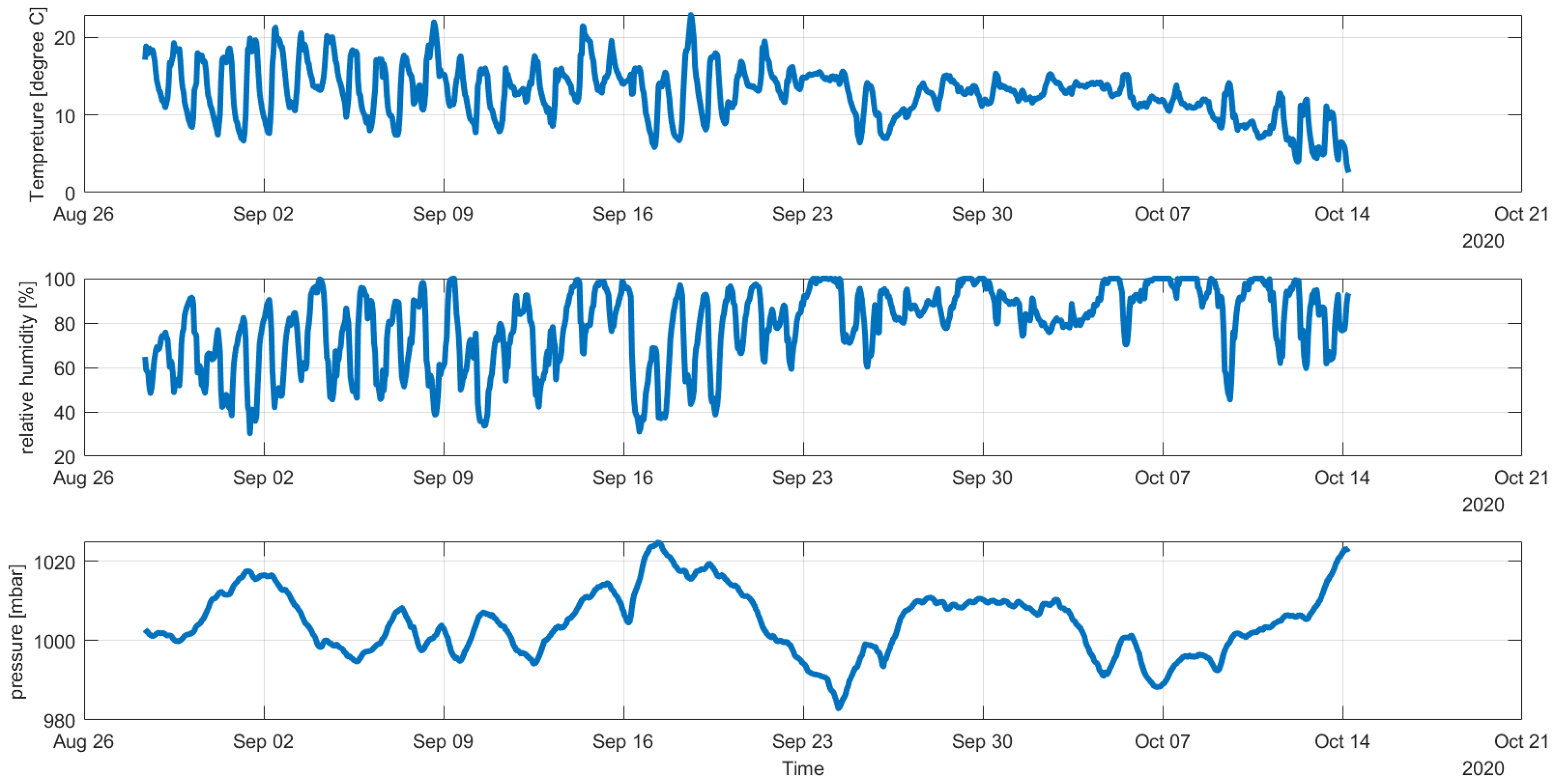
Figure 1 shows the meteorological variability during the measurement period, with air temperatures ranging from 3 to 23 degrees Celsius, with relative humidity between 30% and 100% and atmospheric pressure between 983 and 1029 hPa.

During the co-location period, the hourly particulate matter concentrations measured with the FIDAS instrument varied between 0.5 and 131.5 μg m⁻³ for PM₁₀, 0.2 and 44.5 μg m⁻³ for PM_2.5 and 0.1 and 26.8 μg m⁻³ for PM₁ at the reference station. The higher PM concentrations were measured during the long-range transport episode with hourly maxima of PM₁₀ of 122.2 μg m⁻³, PM_2.5 of 42.9 μg m⁻³ and PM₁ of 22.1 μg m⁻³.

2.3. Sensor Systems

Three commercially available sensor systems were selected for this research: AirSensEUR (https://airsenseur.org/, accessed on 26 July 2021), Ensense (http://www.ensensetech.com/, accessed on 26 July 2021) and Airly (https://airly.org/en/, accessed on 26 July 2021).

Table 1. Characteristics of PM low-cost sensor systems used in the research.

Sensor System	Airly	EnSense	AirSensEUR (ASE)
Manufacturer	Airly, Poland	EnSense, Taiwan	LiberaIntentio, Italy
Approximate price (€)	890	750	870
Dimensions (cm)	16.3 × 8.25 × 7.4	30 × 27 × 18	35 × 32 × 30
Weight (gr)	440	3000	10,000
PM sensor model	Plantower 5003	Sensirion SPS30	Alphasense OPC-N3
Detectable size range (μm)	0.3–10	0.3–10	0.35–40
Estimated PMx concentration	PM10, PM2.5, PM1	PM10, PM2.5, PM1	PM10, PM2.5, PM1

shows their characteristics. The three sensor systems have as output particulate matter mass concentration in the fractions of PM₁, PM_2.5, and PM₁₀. The AirSensEUR system integrates the Alphasense OPC-N3 sensor, which claims to measure single particle counts (http://www.alphasense.com/WEB1213/wp-content/uploads/2019/03/OPC-N3.pdf, accessed on 26 July 2021). Ensense integrates the Sensirion SPS30 sensor, which measures particle density distribution (https://www.sensirion.com/en/environmental-sensors/particulate-matter-sensors-pm25/, accessed on 26 July 2021) and Airly integrates the PM Plantower 5003 sensor, which also measures particle density distribution (http://www.plantower.com/en/content/?108.html, accessed on 26 July 2021). Additionally, the three selected sensor systems also measure temperature and relative humidity. All the units deliver hourly averaged data but Ensense and AirSensEUR can be configured to deliver minute-averaged data. The three units use General Packet Radio Service (GPRS) communication to transfer the data to NILU’s sensor data platform, where it was downloaded through a RestAPI for further analysis.

2.4. Measurement Site Description

For the evaluation, three identical units from each of the sensor systems described above (a total of 9 sensor units) were co-located at the Kirkeveien air quality monitoring station located in Oslo, Norway. The station is categorized as an urban traffic station, as it is close to a street with busy traffic. The Kirkeveien station is equipped with CEN approved gas and PM analyzers. PM₁₀ and PM_2.5 are routinely measured at the station using Tapered Element Oscillating Microbalance (TEOM) (inertial measurement) with a Thermo TEOM (EN12341). For this study, the station was also equipped with a FIDAS 200 (Palas GmbH, Germany) measuring PM₁, PM_2.5 and PM₁₀ fractions and two Kleinfiltergerät (KFG) measuring PM₁₀ and PM_2.5 mass concentrations. The FIDAS provided also temperature and relative humidity data.

The Kleinfiltergerät is an integrated, gravimetric method intended to provide a measurement of either fine particle mass concentration (PM_2.5) or coarse particle mass concentrations (PM₁₀) over a 24 h sampling interval. An ambient air sample is collected by an electrically powered sampler operating at a constant volumetric flow rate. Sample air is drawn from the atmosphere at 38.33 L/min (2.3 m³/h) through an inlet designed to reject insects and atmospheric precipitation and to be insensitive to wind speed and direction. This sample filter is conditioned and manually weighed before and after sample collection to determine the increase in mass. The net mass gain is divided by the measured sample volume to determine the mass concentration of either PM₁₀ or PM_2.5.

The FIDAS is an EN 16450 approved instrument for regulatory measurements of PM₁₀ and PM_2.5. It uses optical properties to determine the particle size and derives the mass from the obtained size distribution and an assumed particle density. The measured particle size distribution is given in 64 bins (from 0.18 μm to 100 μm).

The Thermo Scientific™ 1405-DF TEOM™ Continuous Dichotomous Ambient Air Monitor is a TEOM technique-based instrument. Such monitors measure real-time accumulating mass, as air is drawn through a filter placed on the top of an oscillating glass rod. The air flow rate through the filter is constant and the mass of the particles that attach onto the filter influence the oscillation frequency, which in turn makes it possible to calculate the particle mass and express this per volume of air.

3. Results and Discussion

3.1. Data Preparation

For the purpose of this research, data registered from 28 August 2020 to 19 October 2020 were used. We employed the sensor outputs related to PM₁₀, PM_2.5 and PM₁ mass concentrations (in units of μg m⁻³) as provided by the manufacturer. Our interest in this research is to characterize “out-of-the-box” PM data offered by commercially available sensor sytems, and for that purpose it was assumed that factory-calibrated PM outputs, determined by the manufacturer, should reflect PM concentrations in the best way.

Sensor data were analyzed at two time scales, namely 1 h and 24 h averages. Those aggregation levels are the ones usually employed to inform the public about air quality, and they are also related to the air quality guidelines and thresholds for health protection defined by the WHO (https://www.who.int/news-room/fact-sheets/detail/ambient-(outdoor)-air-quality-and-health, accessed on 26 July 2021) and the EU Air Quality Directive [23].

3.2. Comparison of Optical and Gravimetric Reference Equipment

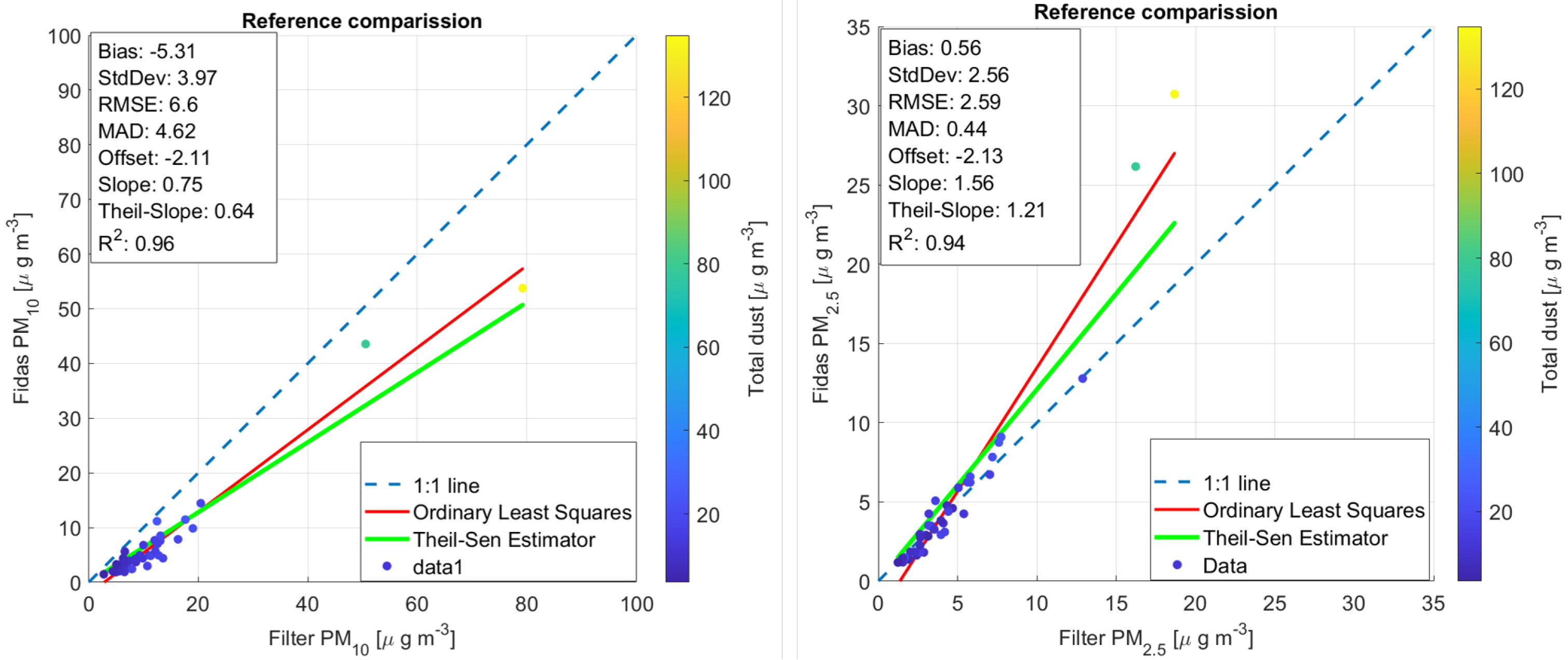
As mentioned before, during the co-location period, we employed optical and gravimetric reference instrumentation. Figure 2 shows the results of comparing both the reference method and reference-equivalent method (Fidas, TEOM) for PM₁₀ and PM_2.5, respectively. The comparison for PM₁₀ illustrates that both methods have a good agreement with a coefficient of determination of 0.96. However, the optical method (FIDAS) underestimates PM₁₀ concentrations. In the case of PM_2.5, both reference methods have a good agreement (R² = 0.94) but the optical method tends to overestimate the PM_2.5 concentrations. This observed underestimation of PM₁₀ and overestimation of PM_2.5 is larger during the two days with higher PM concentrations (marked in green and yellow) that occur during the long range transport episode.

Differences between concentrations measured by optical and gravimetric methods were also found in previous studies. For example, Wanjura et al. [24] found a significant positive linear correlation between total suspended particles (TSP) concentrations measured by collocated TEOM and gravimetric samplers but observed that, in general, the TEOM sampler measured lower concentrations than the collocated gravimetric TSP sampler.

3.3. Time Series

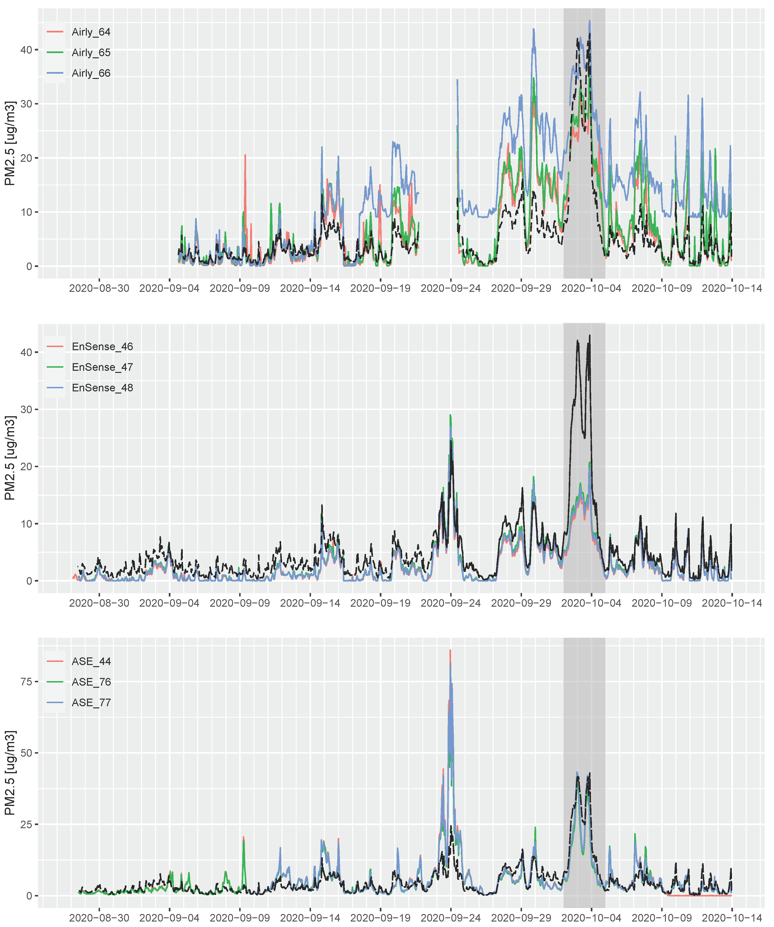
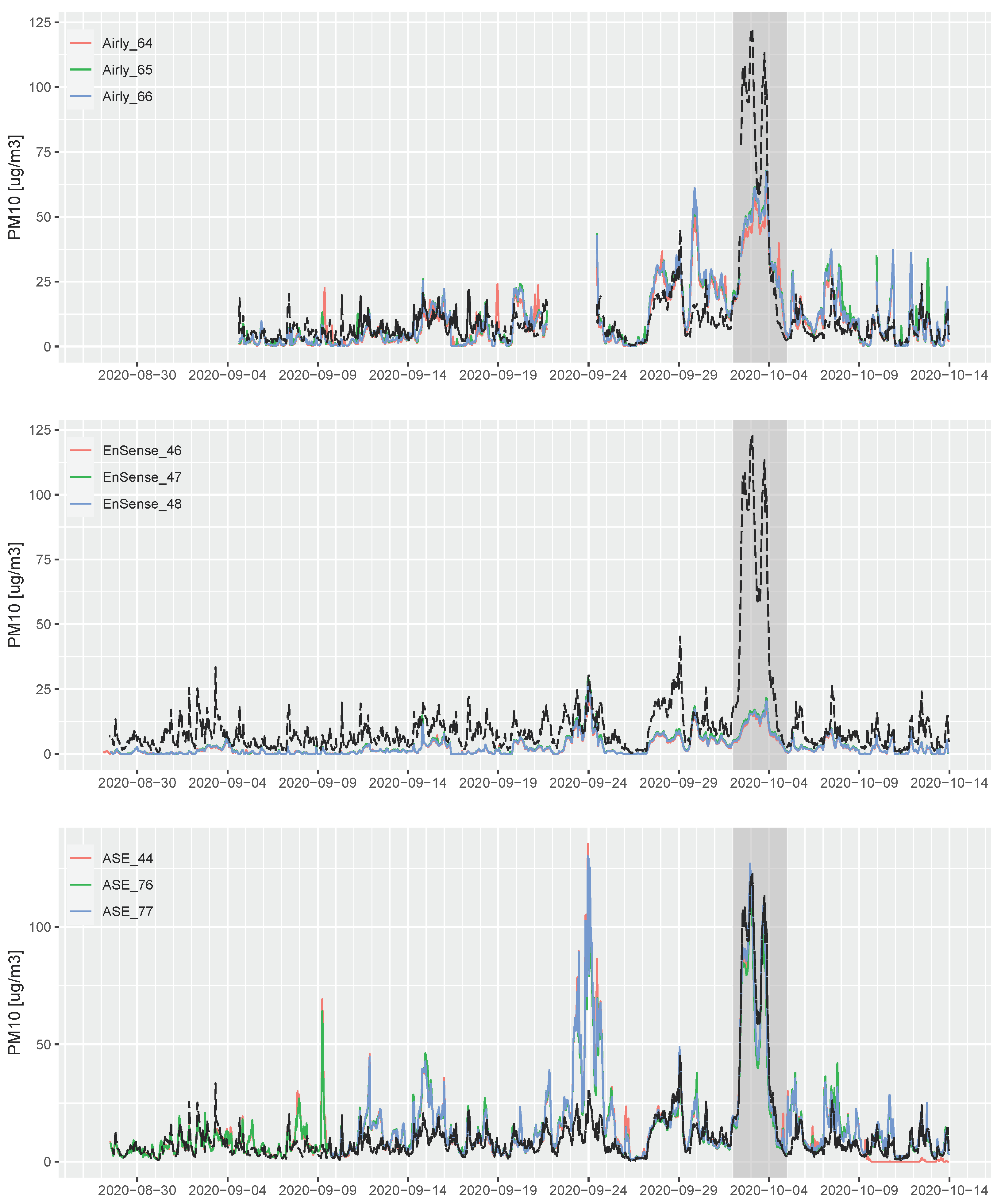
Figure 3 and Figure 4 show respectively the time series of PM_2.5 and PM₁₀ for the 9 sensor systems over the entire co-location period. They also show how these time series vary in relation to the data from the reference instrument. In general terms, we can see that, with exception of the EnSense system, both PM_2.5 and PM₁₀ tend to be overestimated, compared to the reference.

For PM_2.5, all three Airly systems are relatively close to the reference until ca. 15 September, after which all three units provide significantly higher measurements than the reference. From 5 October, two of the Airly systems show again better agreement with the reference data, while one (Airly_66) keeps overestimating PM_2.5 concentrations. The EnSense systems underestimate the actual PM_2.5 concentrations throughout the study period; however, they follow the temporal variability of the reference instrument quite well, with the exception between 2 and 4 October (long-range transport episode), when the sensor systems significantly underestimate the true PM_2.5 concentrations. Finally, the PM_2.5 measurements by the AirSensEUR (ASE) systems in general follow the reference observations well but severely overestimate them around 24 September.

As for PM₁₀, the situation is quite similar with the exception of the Airly sensor showing less of an overestimation as for PM_2.5. EnSense systems underestimate PM₁₀ concentrations, especially between 2 and 5 October. The ASE systems have, in general, good agreement with the reference observations, including the high pollution episode in 2–4 October (long-range transport episode), but similar to what they did for PM_2.5, severely overestimate PM₁₀ concentrations around 24 September. During that day, the meteorological conditions show a drop in the atmospheric pressure and a relative humidity of 100% (see Figure 1).

3.4. Inter-Sensor Comparability

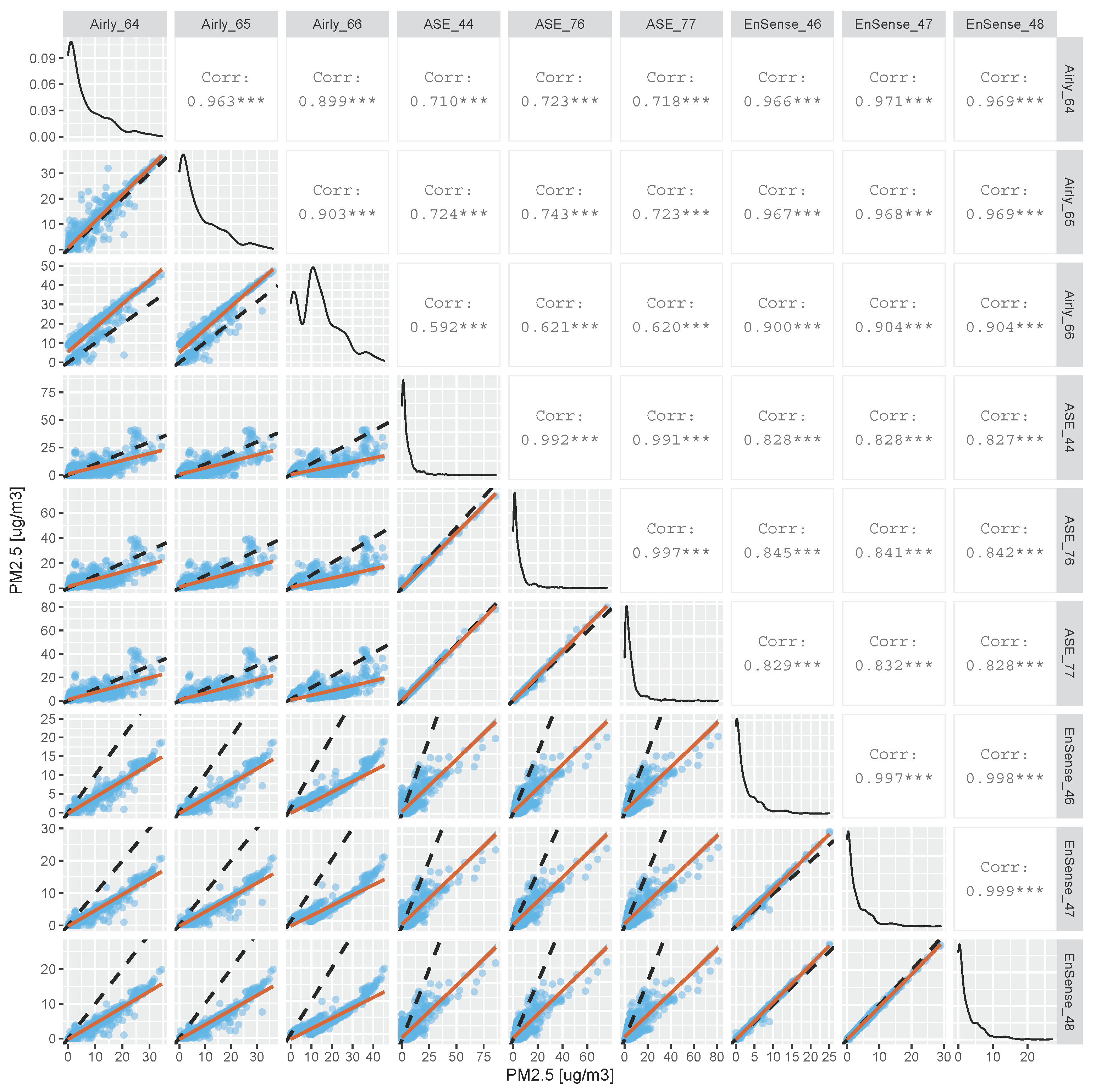
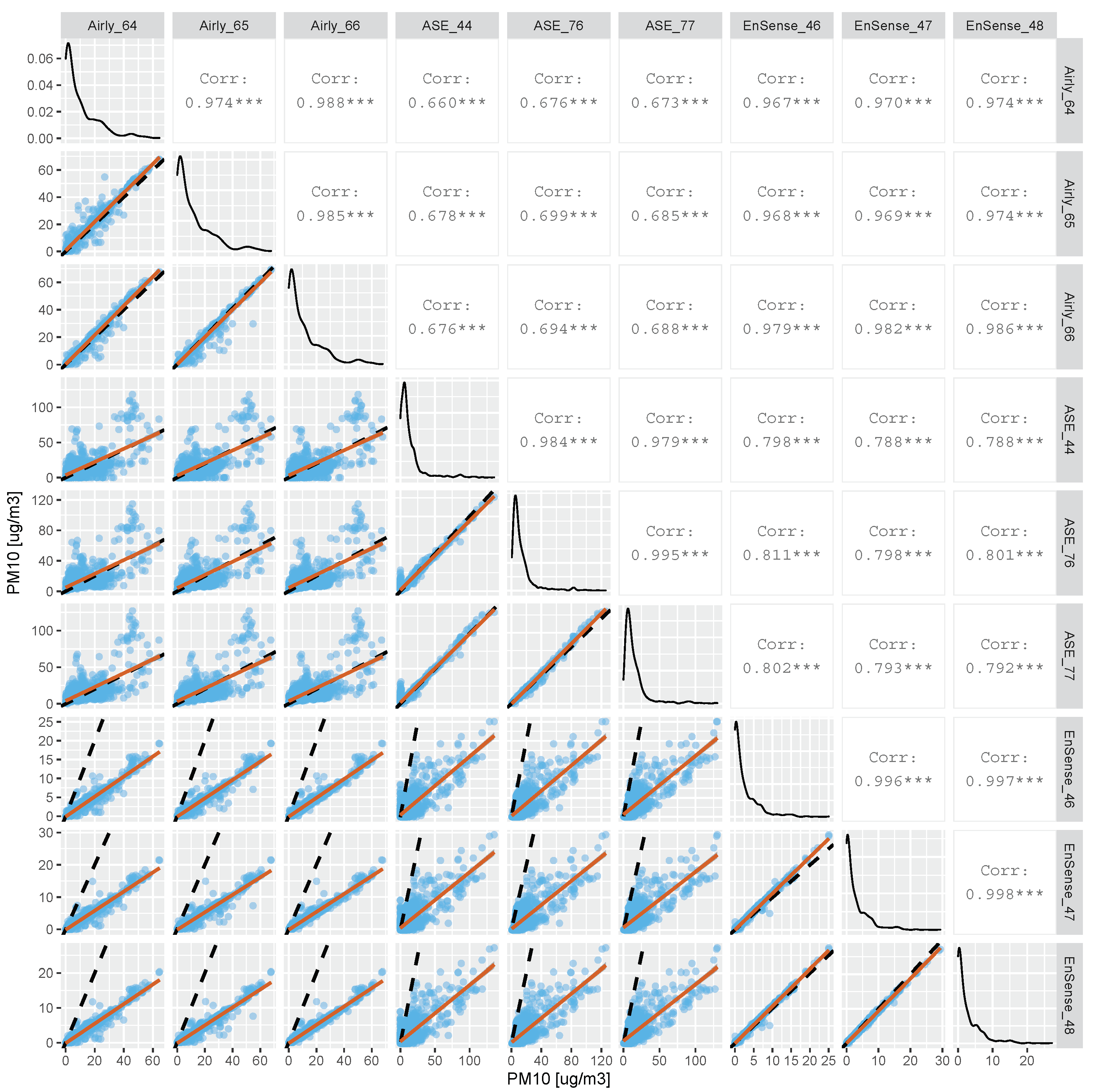
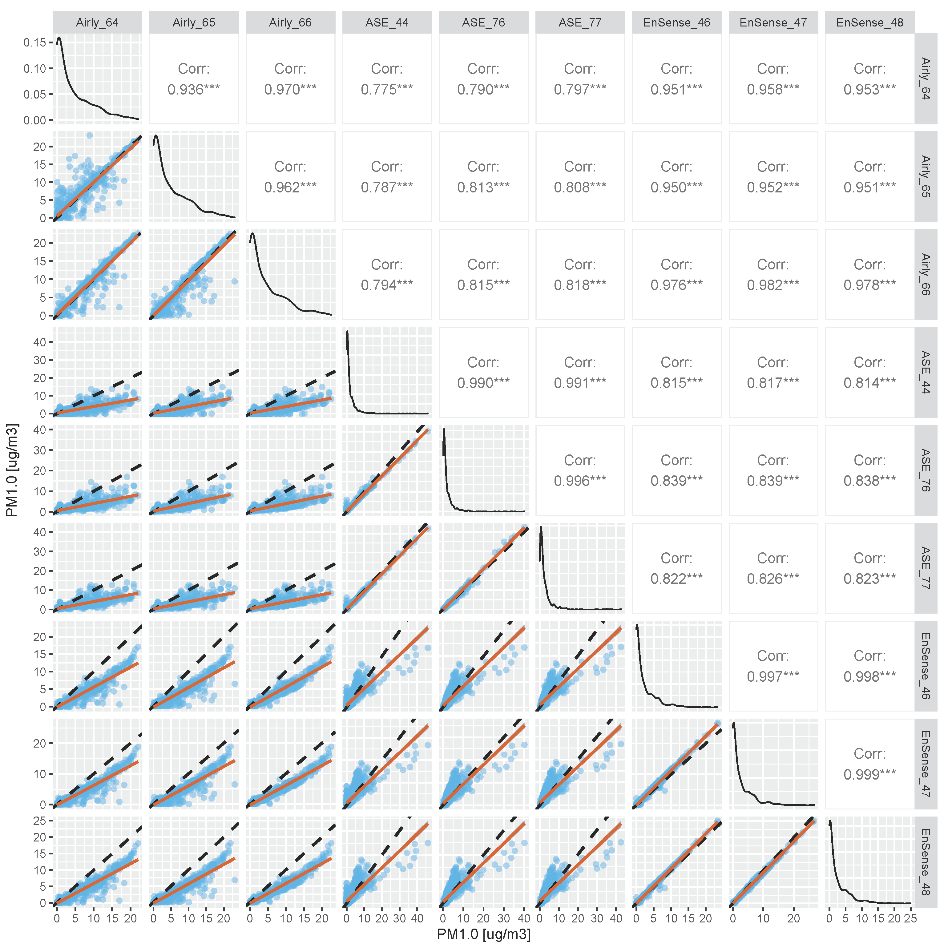
One of the first steps of the co-location study was to evaluate the consistency between individual sensors. This is important because ideally, any potential correction of the data to improve the accuracy should be valid for all sensors. Such an intercomparison between sensor readings can most easily be carried out using a scatterplot matrix. Figure 5, Figure 6 and Figure 7 show this for the factory-calibrated PM_2.5, PM₁₀, and PM₁ signals respectively.

For PM_2.5 (Figure 5) the AirSensEUR and EnSense units exhibit an excellent inter-sensor consistency within each 3-unit group with correlations greater than 0.99. The lowest inter-sensor consistency is displayed by the three Airly units with correlations between 0.89 and 0.96. One of the Airly units clearly shows a significant offset, compared to the other two units. When looking at the correlations between the three manufacturer groups, EnSense units versus AirSensEUR exhibit typically correlations greater than 0.8, however with slopes quite substantially below unity. The comparisons of the AirSensEUR units against Airly exhibit quite a bit of scatter with correlations of 0.59 to 0.74; however, they show slopes very close to unity. In contrast, the scatter plots of the EnSense units against the Airly units display quite good correlations between 0.90 and 0.97; however, the slopes substantially exceed unity.

As for PM₁₀ (Figure 6) the situation looks similar in the sense that both the AirSensEUR units and the EnSense units exhibit an excellent inter-sensor consistency with correlations over 0.99 on average. The three Airly units exhibit slightly more scatter against each other, with correlations around 0.97 to 0.99. In terms of correlations between the three manufacturer groups, for PM₁₀, the AirSensEUR units against the EnSense units show significant scatter (correlation around 0.8) and a slope substantially less than 1. The EnSense units against the Airly units in contrast show a better correlation of over 0.95 but with a slope substantially higher than unity.

For PM₁ (Figure 7) we can observe that both AirSensEUR and Ensense have an excellent inter-sensor consistency with correlations over 0.99. As with the other fractions, the Airly units show more data scatter when compared to each other, which results in correlations around 0.94 to 0.97. In terms of correlations among the different manufacturers, for PM₁ the comparison between Airly and AirSensEUR show correlations between 0.78 and 0.81 and a slope below 1. The comparison between Ensense and AirSensEUR units show also scattered data and correlations between 0.77 and 0.81. The Ensense and Airly units, similar to PM₁₀ and PM_2.5, show less scattered data and higher correlations, with values between 0.95 and 0.98.

The fact that Ensense and Airly units inter-compare better among themselves is most probably related to the fact that both integrate PM sensors (Plantower and Senserion) using the same measuring technique, photometry. The AirSensEUR integrates an optical particle counter (Alphasense OPC-N3). Both methods are based on the principle of light scattering, but the OPC analyzes the light scattered by a single particle, while the sensors based on photometry analyze the light scattered by a cloud of particles. OPCs directly measure the particle number concentration and particle size, allowing the assessment of the particle mass, assuming that the particles are spherical and of a known density. The response of photometers varies not only with PM concentration, but also with particle size distribution, as they are not able to differentiate sizes. This results typically in a biased measurement, as the ambient size distribution typically differs from the size distribution used for calibration.

3.5. Comparison of Sensor Systems against Reference Instrumentation

3.5.1. Comparison of Hourly Averages

Hourly observations from the 9 sensor systems were evaluated against the FIDAS optical reference-equivalent instrument during the co-location period at the Kirkeveien station.

Table 2. Summary statistics of applying the sensor-specific linear regression models to the testing period at Kirkeveien. Reference instrument is Fidas and component is PM₁₀.

	Bias	STD	RMSE	Slope	R2	TSl
ASE44	3.08	12.38	12.75	0.87	0.58	0.88
ASE75	3.6	11.54	12.09	0.84	0.6	0.85
ASE76	4.83	12.76	13.64	0.9	0.64	0.91
EnSense46	−8.44	14.22	16.53	0.15	0.48	0.23
EnSense47	−8.08	14.06	16.21	0.17	0.45	0.27
EnSense48	−8.29	14.16	16.4	0.16	0.46	0.25
Airly64	−1.21	12.35	12.4	0.5	0.54	0.85
Airly65	0.06	12.21	12.2	0.54	0.55	0.97
Airly66	−0.25	12.17	12.16	0.54	0.55	0.94

shows that for PM₁₀, the coefficient of determination varies between 0.45 and 0.64 for all the analyzed sensor systems. The slope is close to 1 for the AirSensEUR systems, but Airly and EnSense have a lower slope around 0.5 and 0.2, respectively. Airly systems have the lower biases (bias below 1.3 μg m⁻³), followed by AirSensEUR (bias ca. 3–4 μg m⁻³) and EnSense (bias ca. −8 μg m⁻³).

For PM_2.5 (

Table 3. Summary statistics of applying the sensor-specific multilinear regression models to the testing period at Kirkeveien. Reference instrument is Fidas and component is PM_2.5.

	Bias	STD	RMSE	Slope	R2	TSl
ASE44	0.57	5.7	5.73	1.01	0.55	0.88
ASE75	0.47	5.03	5.05	0.94	0.57	0.8
ASE76	1.04	6.06	6.15	1.02	0.57	0.89
EnSense46	−2.35	3.65	4.33	0.49	0.73	0.64
EnSense47	−1.97	3.49	4.01	0.55	0.72	0.73
EnSense48	−2.17	3.56	4.17	0.52	0.73	0.68
Airly64	1.37	4.17	4.39	0.91	0.68	1.52
Airly65	2.27	4.41	4.96	0.98	0.68	1.73
Airly66	7.89	6.77	10.39	1.15	0.57	1.95

), the agreement with the reference observations is slightly higher for EnSense and Airly systems, although all the sensor systems have coefficients of determination below 0.75. The linearity for PM_2.5 is higher than for PM₁₀ for all the sensor systems, with slopes close to 1 for AirSensEUR and Airly, but around 0.5 for EnSense. In general, the biases are also lower for PM_2.5 than for PM₁₀, with absolute values below 3 μg m⁻³, except for the unit Airly_66.

The highest correlations between hourly sensor data and reference data are observed for PM₁ (

Table 4. Summary statistics of applying the sensor-specific multilinear regression models to the testing period at Kirkeveien. Reference instrument is Fidas and component is PM₁.

	Bias	STD	RMSE	Slope	R2	TSl
ASE44	2.25	6.2	6.6	1.88	0.59	1.22
ASE75	2.14	5.4	5.81	1.75	0.62	1.11
ASE76	3.02	6.72	7.36	1.92	0.62	1.23
EnSense46	−0.67	0.87	1.1	0.99	0.94	0.9
EnSense47	−0.3	1.1	1.14	1.13	0.94	1.04
EnSense48	−0.5	0.94	1.06	1.06	0.94	0.97
Airly64	3.19	4.18	5.26	2.02	0.9	2.14
Airly65	4.09	4.7	6.23	2.17	0.91	2.38
Airly66	9.71	7.31	12.15	2.6	0.78	2.67

). Ensense and Airly (except the unit Airly_66) have coefficients of determination above 0.9. For the AirSensEUR systems, the coefficients of determination are around 0.6. Biases are also below 3 μg m⁻³, with the exception of the Airly_66 that has a bias of 9.7 μg m⁻³. The slope is between 1 and 2 for all the units. Ensense units are the ones presenting a slope closer to one, with values between 0.99 and 1.13.

The results show that, for the same sensor system, the agreement against the reference data is usually very similar. However, this is not always the case, and some units have higher biases, which indicates the benefit of testing all the units before deployment to properly correct biases from individual sensor systems.

The sensor characterization shows that PM photometer sensors (Airly and EnSense) have the highest correlations against reference data for PM₁, followed by PM_2.5, and lower correlations for PM₁₀. This characteristic is not shown for OPC sensors (AirSensEUR), where the correlations vary between 0.5 and 0.6 for the three sizes evaluated. Although the PM sensor units evaluated have the capacity to measure PM₁₀, PM_2.5 and PM₁, they have inaccuracies, some of them arising from the measuring method, that need to be correctly characterized. Our study shows that photometric sensors capture very well PM₁ concentrations but struggle to measure PM₁₀. Thus, the use of those type of PM sensors should be restricted to studies where the interest is in lower fractions (e.g., wood burning), and should be used with extra caution where the main emissions are of PM₁₀ (e.g., road dust resuspension).

3.5.2. Comparison of Daily Averages

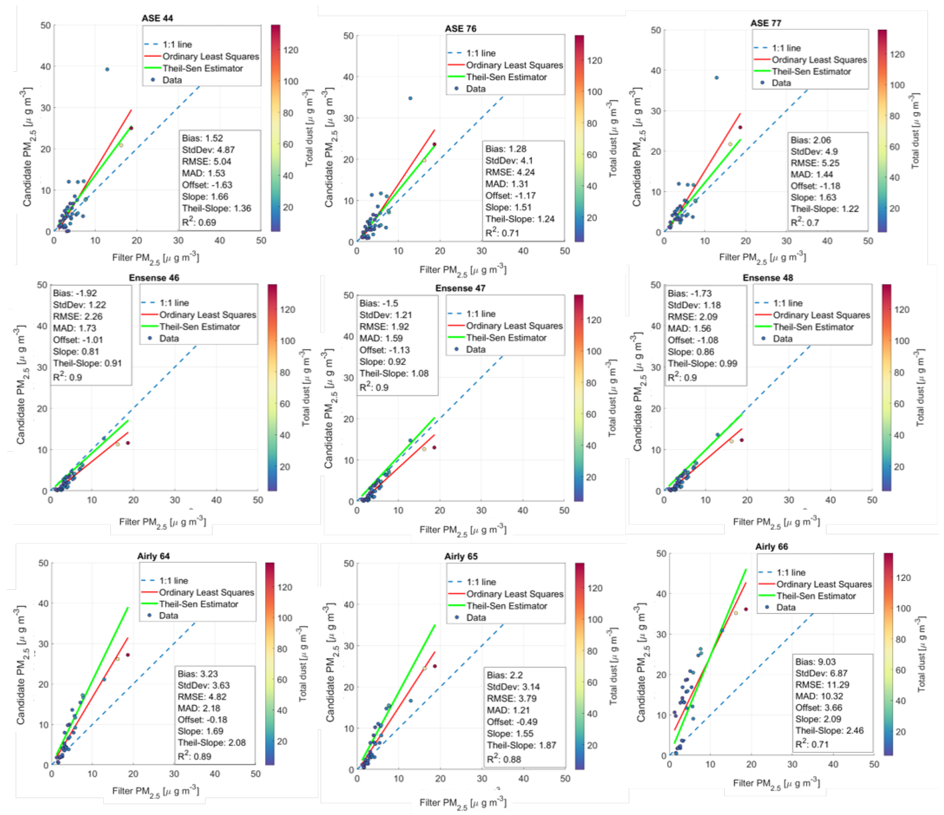
In addition to the hourly characterization of the nine sensor systems against optical reference-equivalent equipment, we also conducted an evaluation of the daily mean observations against the CEN gravimetric reference instrument (Kleinfiltergerät).

Figure 8 shows a comparison between the sensor systems and the KFG for PM_2.5. The Airly and EnSense sensor systems have slightly better correlations (R² close to 0.9, except for the unit Airly 66) than the ASE sensor system (R² = 0.7). The Airly and ASE sensor systems tend to overestimate PM_2.5 concentration, which is shown in a positive bias. The EnSense unit, on the other hand, seems to underpredict the PM_2.5 concentration, resulting in a negative bias around 1.5–1.9 μg m⁻³. The Theil slopes for ASE and EnSense are close to one, while the Theil slope for Airly is close to 2.

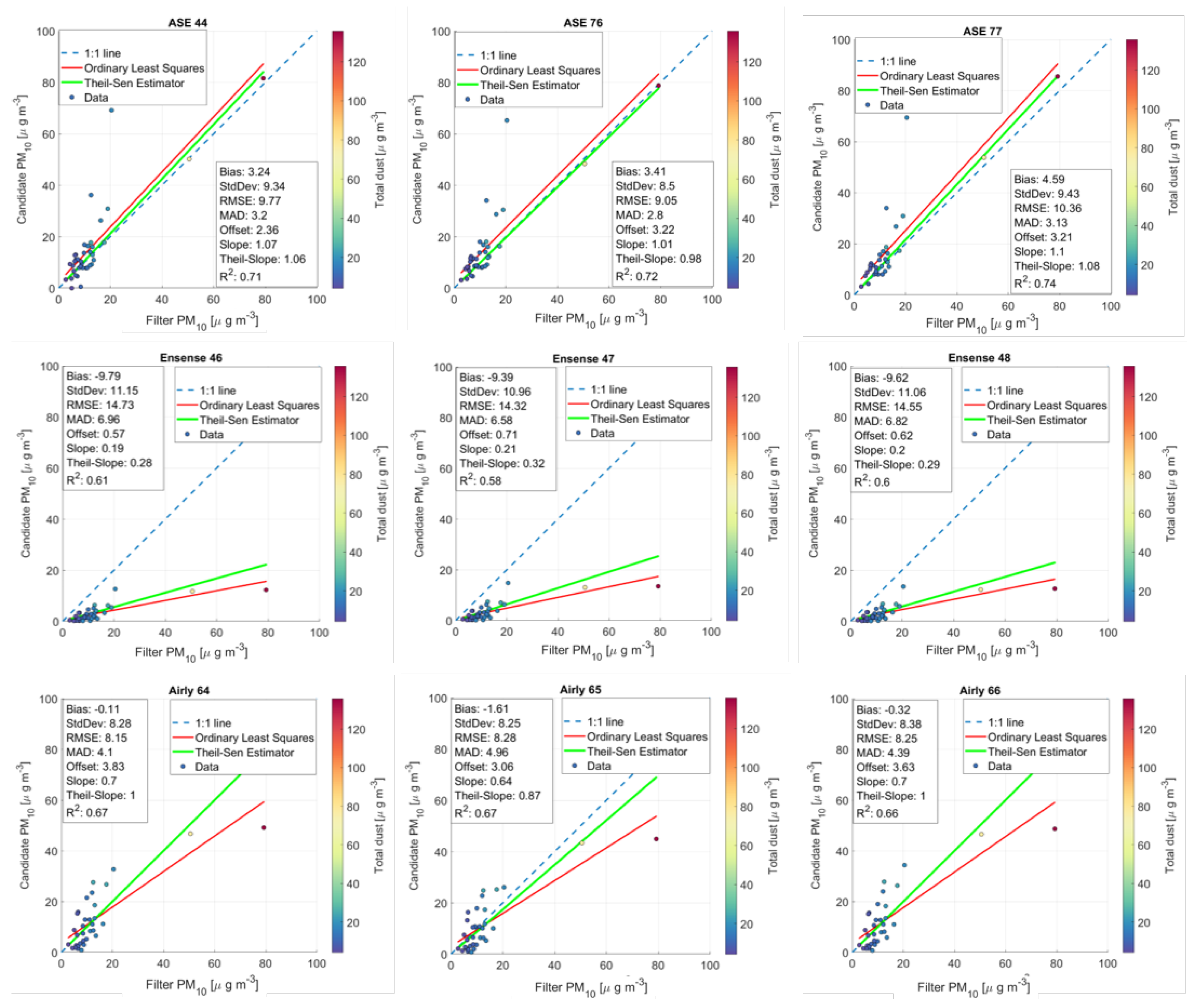
Figure 9 shows the correlation plots of the PM₁₀ measured with the PM sensors systems against the Kleinfiltergeraet. The coefficients of determination vary between 0.6 and 0.7 for all the sensor systems. The Theil slope is close to 1 for the AirSensEUR and the Airly systems, and EnSense has a lower Theil slope of 0.3. EnSense systems tend to underestimate PM₁₀ concentrations resulting in a negative bias around 10 μg m⁻³. The bias for Airly varies between −0.11 and −1.61. The AirSensEUR systems, on the other hand, show a positive bias between 3.24 and 4.59 μg m⁻³.

The results for PM₁₀ are in line with previous research that highlighted the challenges of measuring PM₁₀ accurately with PM sensor systems. Tryner et al. [25] showed that PMS5003 sensors (as the one integrated in the Airly sensor system) were less precise than SPS30 sensors when comparing against reference equipment under laboratory conditions. Kuula et al. [26] tested several PM sensors in the laboratory, concluding that the PMS5003 does not accurately distinguish between PM₁, PM_2.5 and PM₁₀, and cannot be used to measure coarse-mode particles (2.5–10 μm). This is in line with our results, where we found that the most accurate and reliable results are achieved for the PM₁ size fraction.

According to Kuula et al. [26], the ability of PM sensors to measure PM_2.5 with reasonable accuracy depends on the ambient size distribution found in the local environment. For instance, if the ambient size distribution is stable, the PM sensor can be adjusted to measure PM_2.5 [16]. However, there is a risk of data misinterpretation when the sensor measurement is extended to cover particle sizes that it cannot observe. In our study, such limitations of PM sensor systems becomes very pronounced when the size distribution changes in the time period between 2nd and 5th of October, where the PM concentrations were dominated by long range transport of Asiatic desert dust and there was an observed increase in the coarse fraction contribution.

3.6. Long Range Transport of Aerosol and the Effect on Low Cost PM Sensor Systems

Highly elevated PM concentrations were observed during the period between 2nd and 5th of October (Figure 3 and Figure 4). PM₁₀ and PM_2.5 concentrations reached over 120 μg m⁻³ and over 40 μg m⁻³ in Oslo, respectively, while rural background PM₁₀ concentrations reached 97 μg m⁻³ [27]. These concentrations are far greater than any other measured during the co-location period and are among the highest measured in the reference stations in Oslo and in Norway during the last years.

The size of this event compared to the climatological norms, coupled with the spatial extent of the episode covering southern Norway, indicates an origin resulting from long range transport. The examination of the Copernicus Atmospheric Monitoring Service (CAMS) regional ensemble [28] and global data indicates a significant influence of crustal dust transported over southern Norway originated in the region to the east of the Caspian Sea in the Karakum and Aralkum deserts in Turkmenistan and Kazakhstan. In addition to the dust, there was also a series of large wildfire events that occurred in eastern Ukraine that also injected pyrogenic PM into the same weather pattern transporting air north westward of Norway. In addition to the CAMS modeling products, the results from chemical analysis of PM filter samples taken at rural background monitoring sites in Norway showed a large contribution to the high PM₁₀ levels from the coarse fraction (Groot-Zwaaftwink et al., in submission), which was attributed mostly to mineral dust. Evidence was also found of a significant contribution of wildfire smoke to the more minor fine fraction.

During this period, the contribution of particles larger than 2.5 μm in size on the overall mass of PM₁₀ increased from an average of about 5.7 μg m⁻³ to 47.1 μg m⁻³. The performance of the sensor units integrating photometric PM sensors (Airly and Ensense) was heavily affected during the long range transport episode, where PM₁₀ was largely underestimated (Figure 9). Kuula et al. [26] already indicated that the PMS5003, as the one integrated in the Airly sensor system, cannot be used to measure coarse-mode particles (2.5–10 μm). The SPS30 PM sensor integrated in the EnSense unit provides 4 size bins (0.3–1.0 μm, 1.0–2.5 μm, 2.5–4.0 μm, and 4.0–10 μm), which was shown by [26] to be nearly identical, with valid detection ranges of approximately 0.7–1.3 μm. This explains why there is very little variation in the PM₁₀ output during the co-location period, showing similar values for the long range transport episodes, compared to the rest of the measuring period (below 15 μg m⁻³ daily means).

The AirSensEUR sensor system, on the other hand, integrated an Alphasense N3 OPC. The N3 OPC measures, according to the manufacturer, single particles counted in 24 size bins. Unlike most OPCs the N3 OPC does not include a pump to draw aerosol samples through a narrow inlet tube, resulting in a very low sample flow rate of 280 mL/min produced by a micro fan [29]. The N3 OPC captures the long range transport very well, only slightly overestimating PM₁₀ concentrations (Figure 9). This is surprising, as for the rest of the co-location period, the AirSensEUR only shows a moderate coefficient of determination (0.5-0.6) against the reference instrumentation. Other evaluations also corroborate that the N3 OPC has difficulties in measuring PM₁₀ correctly, e.g., [17,30,31,32].

3.7. Evaluation of the Dependency on Relative Humidity

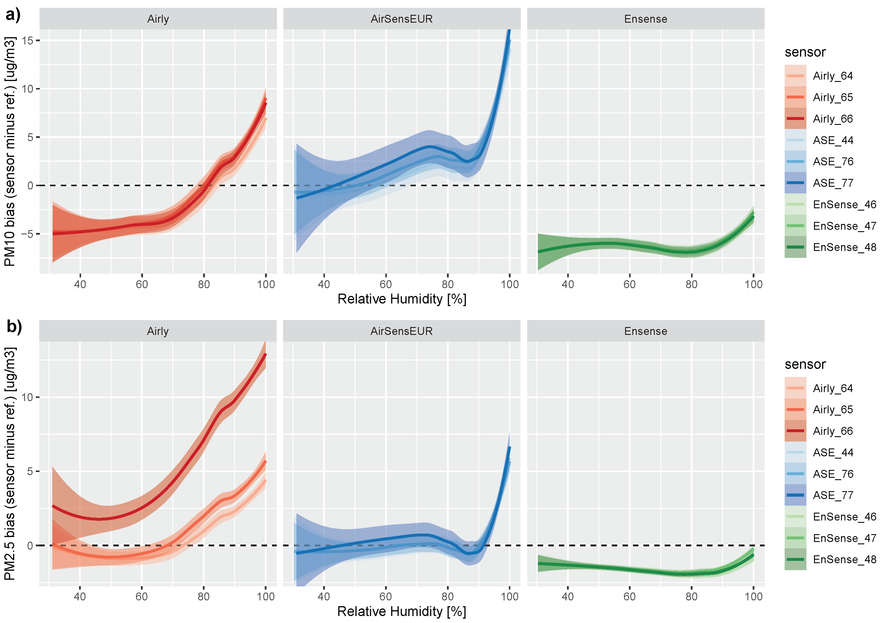
It was shown that low-cost PM sensors can be affected when operating under non-optimal humidity conditions as specified by the sensor manufacturer (usually above 70 percent relative humidity), which results in an overestimation of the actual PM concentration, e.g., [33,34]. Figure 10 shows the relationship between the three tested sensor systems and relative humidity during the co-location period. Similar trends can be seen for individual sensor units from the same manufacturer on PM₁₀ and PM_2.5. The Airly systems, with the integrated PM Plantower 5003 sensor, show a strong change in bias for relative humidity exceeding 70 percent. The EnSense sensor systems, with the integrated Sensirion SPS30 PM sensor, show a small change in bias for relative humidity when exceeding 85 percent, whereas the ASE sensor systems, with the integrated Alphasense N3 OPC, show a significant increase in bias as relative humidity increases and a very sharp change toward positive bias for relative humidity exceeding 90 percent.

The commonly used explanation for this within the sensor community is that this error occurs because the low-cost PM sensor measures in ambient conditions, compared to reference instrumentation, which measures dry particle concentration [33]. This ambient versus dry condition sampling is usually confused with the hygroscopic growth of particles and the resulting positive bias due to larger particles in the sampling system. However, in nephelometry, this error is not due to hygroscopic growth but rather due to a change in light intensity caused by the humidity in the sampling system. Similar to organic compositions or black carbon, water absorbs infrared radiation and can cause an overestimation of particle mass concentrations due to the reduced light intensity received by the phototransistor [35].

The key parameter to describe the influence of RH on the aerosol light scattering is the scattering enhancement factor $f(RH,\lambda )$.

$$f(RH,\lambda )=\frac{{\sigma }_{sp}(RH,\lambda )}{{\sigma }_{sp}\left(R{H}_{dry}\lambda \right))}$$

(3)

where ${\sigma }_{sp}(RH,\lambda )$ is the scattering coefficient at a defined RH and wavelength $\lambda$ and ${\sigma }_{sp}\left(R{H}_{dry}\lambda \right)$ is the corresponding dry scattering coefficient. $f(RH,\lambda )$ will increase with increasing RH and will usually be larger than 1, if the particles do not experience significant restructuring when taking up water [35,36].

Given the results obtained from the three different low cost sensor systems, only the one from EnSense seems to have solved the RH dependency in their out-of-the-box solution. This might be either related to the nephelometer integrated in the solution, or the calibration algorithms from the sensor system provider.

4. Conclusions

Individual sensor systems from the same manufacturer have, in general, good consistency between them, which means that corrections of the data to improve their accuracy should be valid for all sensors without the need to co-locate all individual sensors. However, sensor systems from different manufacturers do not always exhibit similarly good correspondence when inter-compared. We have observed that sensor systems using the same measuring technique (photometry, i.e., Airly and Ensense) compare better among themselves than when compared with sensor systems, using a different measurement technique (optical particle counter, i.e., AirSensEUR).

The results from the evaluation from the nine sensor systems against an optical reference-equivalent instrument (FIDAS 200) showed that the highest correlations between hourly sensor data and reference data are observed for PM₁. The sensors using photometry have coefficients of determination above 0.9, while the sensors using OPC have coefficients of determination of 0.6. PM_2.5 is not as well captured by the sensors as PM₁, and all the analyzed sensor systems have coefficients of determination below 0.75. The units using the OPC N3 have the lowest correlations. All the sensor units have difficulties in correctly measuring PM₁₀, and the coefficient of determination varies between 0.45 and 0.64. Thus, the results of those type of PM sensors should be used with extra caution where the main emissions are coarse particles contributing to the PM₁₀ concentrations (e.g., road dust resuspension, construction including road work, demolition, etc.).

The results from the comparison of daily mean observations against the CEN reference (Kleinfiltergerät) instrument corroborates that the PM sensor systems can measure PM_2.5 but struggle to measure PM₁₀. The units using photometry (Airly and Ensense) have slightly better correlation (R² = 0.9) than the sensor system using OPC (AirSensEUR) (R² = 0.7). For PM₁₀, the coefficient of determination varies between 0.6 and 0.7.

The comparison against reference instrumentation also shows that, for the same sensor system, the agreement against reference data is usually very similar. However, this is not always the case, and some units have higher biases, which indicates the benefit of testing all the units before deployment to properly correct biases from individual sensor systems.

The ability of PM sensors to measure PM with reasonable accuracy is linked to the ambient size distribution found in the local environment. For instance, if the ambient size distribution is stable, the PM sensor can be calibrated. In our study, such limitations of PM sensor systems becomes very pronounced when the size distribution changes in the time period between 2nd and 5th of October, where the PM concentrations were dominated by long range transport of desert mineral dust. During this period, the contribution of particles larger than 2.5 μm in size on the overall mass of PM₁₀ increased from an average of about 5.7 μg m⁻³ to 47.1 μg m⁻³. The performance of the sensor units integrating photometric PM sensors (Airly and Ensense) was heavily affected by this, and PM₁₀ was largely underestimated.

When evaluating the dependency with relative humidity, the results show that the analyzed sensor systems have different responses to the variation of the relative humidity. The errors are due to the change in light intensity caused by the RH in the sampling system. We observed that only EnSense seems to have solved the RH dependency in their out-of-the-box solution. This might be either related to the nephalometer integrated in the solution, or the calibration algorithms from the sensor system provider. The Airly systems, with the integrated PM Plantower 5003 sensor, show a strong change in bias for relative humidity exceeding 70 percent, whereas the AirSensEUR sensor systems, with the integrated Alphasense N3 OPC, show very sharp change for relative humidity exceeding 90 percent.

The sensor systems evaluated in this study show good agreement with reference instrumentation for PM_2.5, particularly those using photometry as a measuring technique. However, they might have difficulties to correctly capture PM_2.5 concentrations when the ambient size distribution is different from the one that the sensor system has been calibrated for. This was the case during the long-range transport event. All the sensor systems struggled to measure PM₁₀, posing a risk of misinterpretation of the data when the sensors are used to monitor such a particle size.