Assessment of Climate Variability among Seasonal Trends Using In Situ Measurements: A Case Study of Punjab, Pakistan

Abstract

This research assessed the changes in spatial patterns and the seasonal trends in temperature, precipitation, and relative humidity over 36 years (1979–2014) using Climate Forecast System Reanalysis (CFSR) datasets. The evaluation of climate deviations was the prime objective of this research. The augmented Dickey–Fuller Test (ADF) was used to scrutinize whether the data was either stationary or non-stationary. The results of the ADF test showed that all the datasets were found to be stationary at lag order 3. To observe undulations in the time series data, trend analyses were done using Sen’s slope (SS), Mann–Kendall (MK), and Cox and Stuart (CS) tests. For all the statistical analyses, we considered the 5% significance level (α = 0.05) and p < 0.05 to be statistically significant. We observed significant (p < 0.05) trends in spring (MAM) and autumn (SON) for minimum temperature (T_min) in Punjab. We also noted a significant (p < 0.05) trend in precipitation during autumn (SON). Annually, all the variables showed a non-significant (p > 0.05) trend for Punjab, Pakistan, during the period 1979–2014. Climate variability, such as a decrease in precipitation, higher temperature, and relative humidity fluctuations, were the reasons for the imbalance in the sustainability of Punjab, Pakistan.

1. Introduction

Globally, climate change has a profound impact on many areas due to the variability in temperature and precipitation. It has attracted significant attention from researchers during the past few decades [1]. Climate change has become an emerging issue in some regions in recent years. It was demonstrated by various researchers [2] that the recorded fluctuations in temperature, precipitation, and relative humidity in the current era happened not only because of natural phenomena but also due to anthropogenic activities. The global mean surface temperature (GMST) increased by approximately 0.72 °C during 1951–2012 [3]. Correspondingly, there was a 2% increase in the proportion of universal land precipitation [4]; variations in precipitation patterns have ultimately impacted Pakistan’s water reserves and agriculture [5]. Being an agriculture-dependent country, Pakistan is under climate threat. The 2000s was known as the warmest decade, and 2016 was known to be the warmest year of the last century in Pakistan. During the past three decades, the observed T_mean ranged from 0.78 to 1.5 °C, and at the end of this century, it is estimated to be 2 to 4 °C according to the warming trend of the climate [6,7,8]. Rising temperatures are expected to have a significant impact on arid and semi-arid research regions in Punjab, Pakistan, such as Nankana Sahib, Sialkot, Multan, and Gujranwala [9].

Furthermore, temperature, precipitation, and relative humidity are synchronized with nature and reveal homogenous changes. For instance, an enormous amount of calculations is available regarding climate variability, but temperature, precipitation, and relative humidity are consequential indicators. Their annual and seasonal changes can help to study the alterations in climate [10]. The increase in temperature (such as T_max, T_min, and T_mean) leads to changes in precipitation and land warming, causing climate variability [11,12,13]. To mitigate these effects, assessment and adaptive measures can be based on the analysis of time series trends [14].

Changes in climate patterns are becoming the cause of droughts. However, reports on the of drought fragility and its numerical appraisal are rare [15]. The convergence of climatic factors and anthropogenic activities is called risk assessment. Therefore, to intensify the rationality of impact assessments, the separation of the degrees of influence of different climatic variables is mandatory. Understanding the relationships between climate variability and anthropogenic activities is critical for forecasting future changes and understanding profound variations and procedures in climate systems [16]. In addition to anthropogenic activities, changes in natural phenomena, such as fewer monsoons, intensified and longer cycles of rains, sea-level rise, cyclones, and tropical storms, have created prolonged droughts in winter and have accelerated the climate system [17,18].

Numerous studies have shown that climate change can cause harm to the accessibility of environmental resources, resulting in an imbalance in sustainability [19]. For example, due to global warming, some species are endangered with extinction [20] because the pressure from climate variability in the tropical forest area has been increasing [21]. The decline in water accessibility is depleting the natural water resources. The above changes are caused by changes in climatic factors (temperature, precipitation, and relative humidity). We explored all these variables in the current study. Establishing an equilibrium in environmental demand and supply under the current changing climate in a timely manner is an arduous task. Some researchers also found that the future climate variability will cause an increase in the persistence and intensity of weather events [22]; this might increase the challenges of environmental reserves in a negative way and, as a result, create an imbalance in ecological sustainability. According to the above-stated limitations, to check climate suitability, expertise-based approaches are frequently used. Multiple parameters, including temperature, precipitation, wind speed, drought, and solar radiation, are under consideration when figuring out the adequacy and usefulness of literature reviews and expert questionnaire surveys. To address these problems, and to understand possible movements in sustainability with climate change, an extensive selection of actions was applied in the past few years [23].

For underdeveloped countries, such as Pakistan, the natural climate is mainly at risk because of urbanization and industrialization. These nations are primarily agriculture-dependent, where this sector is highly vulnerable to climate variability and does not have many sources to adjust to the changing circumstances. In this regard, in such countries, the identification of traditional changes in climate parameters is of prime importance where the pillar of the economy is the agriculture sector, such as in Pakistan. Pakistan is located in one of the regions experiencing a sudden temperature increase [24,25]. The early studies have specified changes in temperature in different parts of Pakistan, such as in the Indus basin, where a significant positive trend has been observed in temperature indices [26]. In contrast, in the northern part of the country, decreasing trends in T_max, T_min, and T_mean were identified [27]. For northern, northwestern, and northeastern regions, research on rainfall trend analysis has found an increasing bias in the annual rainfall [28].

In contrast, starting from the late 1990s, [29] reported a decrease in precipitation and a temperature rise for the many sub-basins in the Upper Indus Basin (UIB). The study used six atmospheric factors in the UIB to estimate the trends that were attributable to the deficiency in the availability of in situ monitoring. Further, through numerous studies in southern and central areas of Pakistan, a decreasing trend in annual rainfall was described [30]. So far, no comprehensive research has been performed related to the spatiotemporal trends of the temperature, precipitation, and relative humidity in various parts of Punjab, Pakistan, which is a highly important region for agriculture [24].

In comparison, the early studies generally did not focus much on the primary components of seasonal trends in climate variability. Many studies showed trends in climate change by using observed data. Using the MK test and Sen’s slope estimator, much literature has identified the temperature fluctuations and precipitation levels in Punjab, Pakistan. A brief review of the climatic trend analysis in Punjab, Pakistan, using different variables is given in

Table 1. A comprehensive outline of the previous studies on the climatic trends of Punjab, Pakistan.

Research	Timescale and Datasets	Study Area	Quality Control of Data	Method	Findings
Iqbal and Ali [34]	Annual (1981–2010) and gauges	Lahore, Murree, Sialkot, Jhelum	Percentile or quantile method, statistical distribution to sort and fit the data into extreme events	GEV distribution, log-Pearson type III analysis, and Gumbel distribution	Daily 100 mm precipitation and more were observed; therefore new dams are needed.
Aslam et al. [35]	Observed and projected (past and future) (2011–2085) and gauges	Southern Punjab	Climatic models and IPCC’s A2 and A1B scenarios	GEVs distribution, CREAT and GIS software	Climate change risks identified.
Khattak and Ali [36]	Annual, seasonal (1961–2014), and gauges	Punjab	TFPW approach used in data	MK test and Sen’s slope	SON and DJF seasons showed the most significant changes of all.
Salma et al. [37]	Decadal (1976–2005) and gauges	30 stations of Pakistan	Not mentioned	ANOVA, Dunnett T3	Rainfall showed a decreasing trend all over Pakistan.
Jahangir et al. [38]	Seasonal, annual (1979–2013), and (ECMWF) (ERA-Interim)	Eight tehsils of Punjab	Not mentioned	Regression, MK test	Tmin had no annual trend.
Abbas [39]	Daily (1981–2010) and gauges	Sargodha, Multan, Faisalabad, Bahawalnagar, Rawalpindi	13 temperature indices concerning semi-arid environments analyzed using RClimDex	Mann–Kendall test, Sen’s slope	Overall warming in regions, as depicted by significant trends in the temperature patterns
Li et al. [40]	Monthly, annual (1980–2011), and gauges	Southern Punjab	Not mentioned	SimCLIM	Sustainable management of climatic risk required.
Abbas et al. [41]	Daily, monthly, annual (1981–2010), and gauges	Five cities of Punjab	RClimDex used to assure that data was error free	MK test, Sen’s slope	No spatio-temporal trends were depicted.
Nashwan et al. [24]	Annual, seasonal (1967–2017), and gauges	Punjab	For the removal of autocorrelation, they used a pre-whitening procedure	Mann–Kendall, Sen’s slope, IDW	Spring was the warm season.

. These studies have some limitations since they analyze only a small proportion of stations or focus on only one or two indicators. As such, it is difficult to comprehend their trends and spatial patterns. Further, most of the early studies used the MK test, which cannot identify the monotonic trends in long-run changes in climatic events.

The newness in current research is that SS and MK are used, along with the CS test, to analyze the temporal and spatial trends in temperature (T_max, T_min, T_mean), precipitation, and relative humidity in Punjab, Pakistan. The current study examined the spatiotemporal changes in temperature trends (T_max, T_min, T_mean), precipitation, and relative humidity for 16 different stations in Punjab, Pakistan. The analysis of climate variability has recognized events in environmental systems that impose some severe threats to human well-being and sustainability [31]. Levin and Clark [32] determined some of the significant challenges and threats to sustainability. They elaborated that because of the current climatic variability, the responses to sustainability challenges are resulting in not conserving natural reserves for future generations but are strengthening adaptability in the ecosystem. Now the question is whether current management is sustainable under a changing climate and whether adjustments are needed [33]. The main objectives of this research were (1) to address the regional measurement of the seasonal trends in the climatic variability of Punjab, Pakistan, and (2) to identify the spatiotemporal heterogeneity in the climate fluctuations of Punjab, Pakistan, using weather stations.

2. Materials and Methods

2.1. Study Area

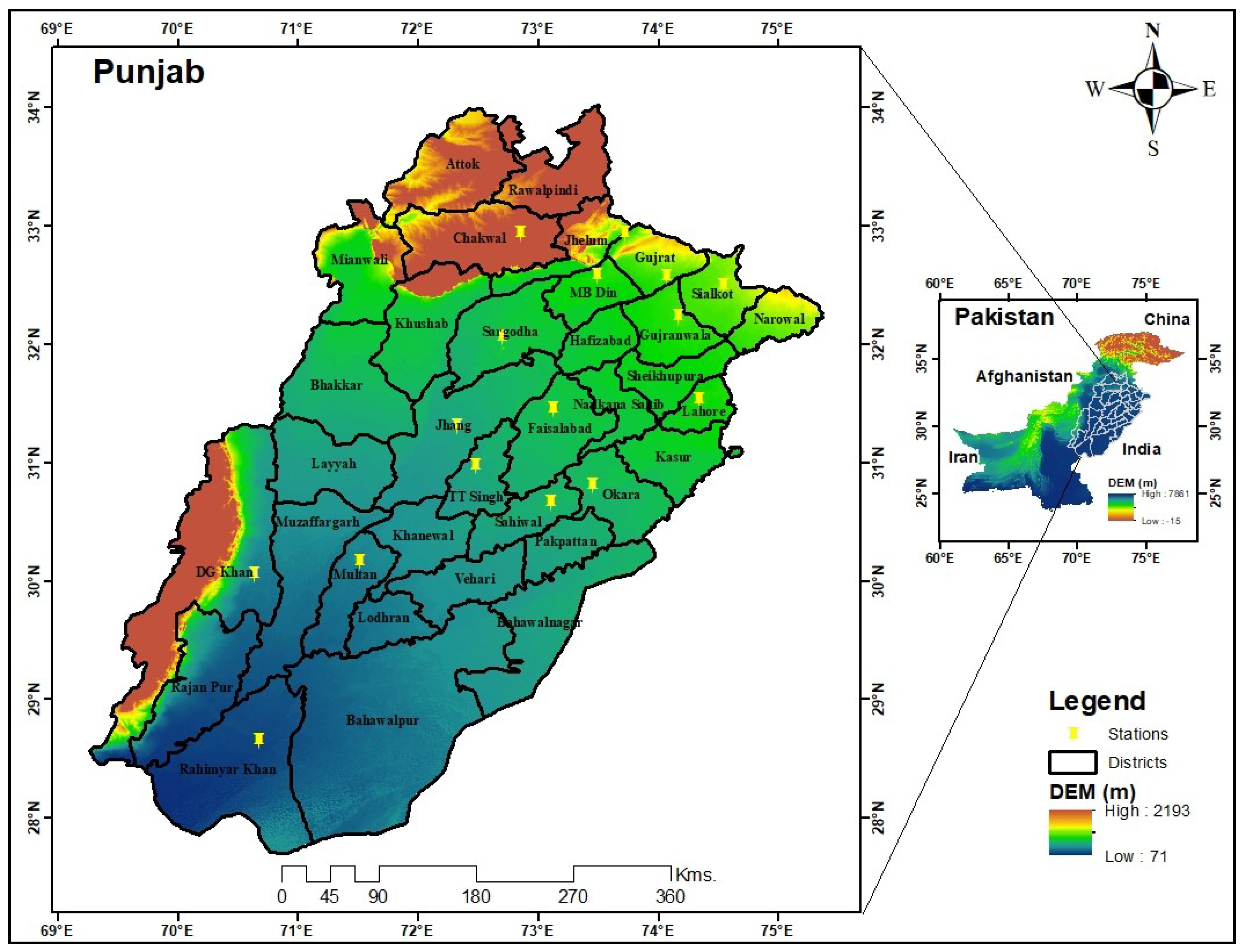
The study area of Punjab is the 2nd largest province of Pakistan among the four provinces (Balochistan, Khyber Pakhtunkhwa, Punjab, and Sind) and is geographically located in between 24–37° N and 62–75° E (Figure 1). Climatologically, most of Punjab is arid and semi-arid, having a finite spatio-temporal variability in the climate indicators, including precipitation; relative humidity; and maximum, mean, and minimum temperatures [42]. More than half (59%) of the annual precipitation is because of monsoons, which are the supreme hydro-meteorological reserve of Punjab. The elevation of Punjab varies between 71–2193 m. From March to May (spring), the temperature rises, and this situation remains until summer [38]. Furthermore, the monsoons are expected to arrive in Punjab at the end of May, although weather conditions have shown unpredictable patterns since the early 1970s.

During 1970–2001 in Punjab, Pakistan, the average annual T_max was generally between 29.3 and 31.9 °C; on the other hand, the average yearly T_min was between 16.3 and 18.2 °C [43]. The rainfall in Punjab is widespread, which is generally connected to monsoon winds. The highest rainfall was received by the rain-fed (Barani) zone and the irrigated plains, marginal land, and Thal region [44]. Altogether, the climate is arid and has an annual precipitation of 100 mm in the south, 600 mm in the northwest, and 1000 mm at the northeastern boundary. The yearly primary precipitation is from the monsoon season from June till September, leading to flooding [45]. The temperature generally ranges between −2 °C and 45 °C, but it can go as high as 47 °C in the summer season, and it can as low as −5 °C during the winter season.

2.2. Land-Cover Type (LC Type)

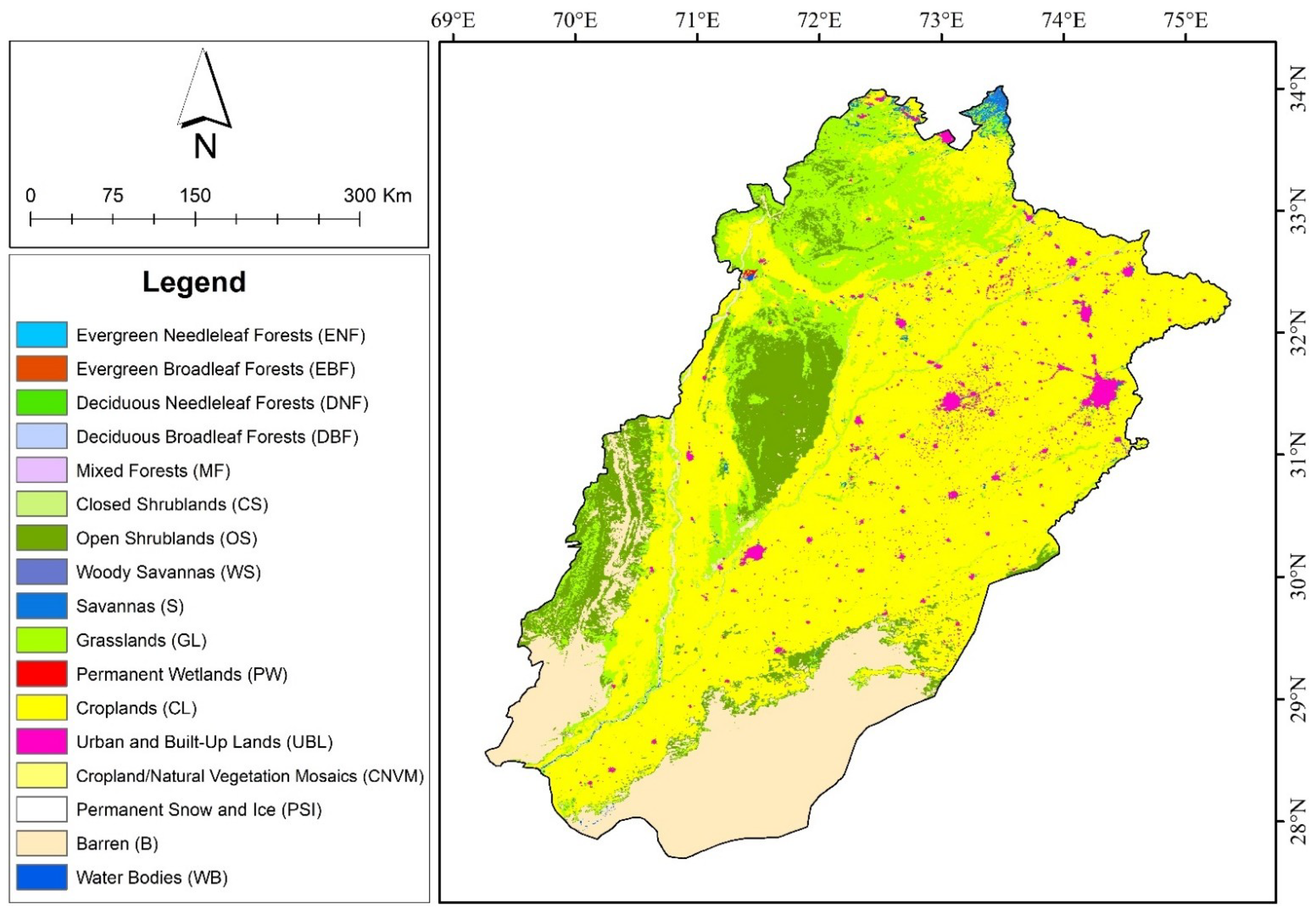
To determine the progressing changes, the LC mapping for a region is an important task. Land-cover mapping helps us discover whether a specific sector, i.e., agriculture or urban, requires proper planning and management. Land-cover descriptions and the area occupied by each LC type for Punjab, Pakistan, are available in

Table 2. Land-cover types of Punjab, Pakistan, that were identified from MODIS (MCD12Q1) images using IGBP classifications [47,48].

LC Type	Area (km²)
Evergreen Needleleaf Forests (ENF)	105.3
Evergreen Broadleaf Forests (EBF)	3.5
Deciduous Needle leaf Forests (DNF)	0.0
Deciduous Broadleaf Forests (DBF)	0.0
Mixed Forests (MF)	0.0
Closed Shrublands (CS)	3.5
Open Shrublands (OS)	21,375.8
Woody Savannas (WS)	70.6
Savannas (S)	1357.7
Grasslands (GL)	28,215.8
Permanent Wetlands (PW)	64.5
Croplands (CL)	115,836.3
Urban and Built-Up Lands (UBL)	3882.7
Cropland/Natural Vegetation Mosaics (CNVM)	64.3
Permanent Snow and Ice (PSI)	0.0
Barren (B)	34,208.6
Water Bodies (WB)	155.5

. Punjab, Pakistan, has 5 major rivers: Ravi, Sutlej, Jhelum, Bias, and Chenab. These rivers carry sediments that arise due to swift erosion from the Himalayan south mountains into the Indus River Delta and then into the Arabian Sea [46]. The LC type data of Punjab, Pakistan, that were identified from MODIS (MCD12Q1) images using IGBP classifications are shown in Figure 2 and Table 2.

2.3. Data Source

This study used data from 16 stations in Punjab, Pakistan, to assess the climate vulnerability. The Climate Forecast System Reanalysis (CSFR) data were used in this research. Daily data from 1979 to 2014 for 16 stations were downloaded from the Global Weather data for SWAT (https://globalweather.tamu.edu/, last access: 10 September 2014) website. It was used to investigate the long-run variability in the seasonal and annual maximum, minimum, and mean temperature, precipitation, and relative humidity. The studied stations are located in various irrigation zones of Punjab, Pakistan, and daily data for 5 variables were used in the current study, as shown in

Table 3. Information about the studied stations in Punjab, Pakistan.

Station	Latitude (N°)	Longitude (E°)	Altitude (m)
Chakwal	32.94	72.81	518
DG Khan	30.13	70.62	122
Faisalabad	31.46	73.13	172
Gujranwala	32.32	74.15	225
Gujrat	32.62	74.06	230
Jhang	31.37	72.18	156
Jhelum	32.94	73.75	222
Khanpur	28.65	70.62	76
Lahore	31.69	74.37	205
MB Din	32.62	73.43	208
Multan	30.13	71.56	118
Okara	30.75	73.43	164
Sahiwal	30.75	73.12	160
Sargodha	32.00	72.81	177
Sialkot	32.62	74.68	255
TT Singh	30.06	72.48	163

. We selected these 16 stations due to their popularity and the completeness of records based on their spatio-temporal coverage, history, and uniformity. The considered seasons are described as follows: winter (December, January, February (DJF)), spring (March, April, May (MAM)), summer (June, July, August (JJA)), and autumn (September, October, November (SON)) [49].

3. Used Techniques

For the trend analysis, three types of techniques were used in this study. Before the Mann–Kendall (MK), Sen’s slope estimator, and CS methods can be used, it is mandatory to test whether the time series datasets are stationary. To analyze the stationarity of the datasets, there are many methods, but in this study, we used the augmented Dickey–Fuller test (ADF) for T_max, T_min, T_mean, precipitation, and relative humidity data series in RStudio. Because the results for the unit root testing were reliable, the ADF test was a good option, as it can perform a more significant number of observations, especially in the case of a time series [50]. Due to its simple assembly and feasibility, it is the most regularly used test. Furthermore, the trends analysis was done using the MK test, Sen’s slope estimator, and CS methods. Rather than comparing the data values themselves, the MK test compares the similar magnitudes of the sample datasets [51].

One boon of this test is that there is no need for the data to fit a certain distribution. A second benefit of the test is available, which is its low sensitivity toward quick breaks because of an inhomogeneous time series [2,52]. CS [53] defined it as a little powerful test, but it is very rigorous regarding trend analyses. The method we discussed is based on the binomial distribution, and it can be applied to an extensive range of conditions. This method was used to verify the significance of the trend and establish the magnitudes of variability and directions of changes. The technique is more helpful for detecting magnitude and direction when the Mann–Kendall test is used [54]. SS regulates the magnitude of a present trend [55]. In this study, these techniques were used to assess the patterns of the variables and their significance levels in Punjab, Pakistan. Moreover, for investigating the atmospheric dynamics of Punjab during the study period, geopotential height data of 850 hPa for 1979–2014 and latitudes of 0–60° N and longitude 40–100° E were retrieved from NCEP/NCAR and analyzed. This dataset was developed in a three-state reanalysis with a spatial resolution of 2.5° × 2.5° latitude by longitude and a 4 h temporal resolution (00, 06, 12, and 18).

3.1. Augmented Dickey–Fuller (ADF) Test

Through ordinary least squares (OLS) regression models, the Dickey–Fuller unit root tests incorporate a linear trend. Suppose the following AR (1) model [56]:

$$X_t=\rho X_{t-1}+{\rho }_t, t=1;2;\dots .; n$$

(1)

where $X_0=0,$ $\left|\rho \right|\le 1$:

$$\widehat{\rho }={\left[{\displaystyle \sum }_{t=2}^n{X}_{t-1}^2\right]}^{-1} {\displaystyle \sum }_{t=2}^n{X}_t{X}_{t-1}$$

(2)

The statistic to check the null hypothesis, p = 1, depends on a common OLS (ordinary least squares) t-test:

$$\frac{t=\widehat{\rho }-1}{{\widehat{{\rm Y}}}_{\widehat{\rho }}}$$

(3)

The augmented Dickey–Fuller (ADF) stationarity test was first proposed by [57] and modified by [58] and is used to detect whether the data has a unit root. The augmentation can be done in the standard autoregressive unit root test (referred to as the ADF test) to assist general AR (p, q) models with unspecified orders [56]. The DF procedure, which was organized for the auto-regression presentations of familiar orders, remained asymptotically viable for a common ARIMA (p, 1, q) approach for p and q that are of unspecified orders.

3.2. Mann–Kendell (MK) Trend Test

In the current research, we used the Mann–Kendall (MK) test to undertake trend analyses. This test is also known as a distribution-free (non-parametric) test. It is rigorous regarding missing values and is less sensitive to the swift breakpoints [59]. In hydrological or metrological temporal data series, it has a universal use since it can detect whether a trend is available in either dataset [60]. Nevertheless, the test is prone to the serial correlation that may influence the results [61]. In the present research, before proceeding to MK to probe the analytical magnitude and significance of the trends in the datasets, the sequential correlation approach was employed for the series.

MK test was used to analyze the changes and whether they were significant. The MK test can be applied to detect trend analysis because it only requires the assumption of independent datasets, though the chance of a significance level in the trend can be increased by the availability of serial autocorrelation in datasets [62]. Past research expressed that significant trends with time are also sensitive toward autocorrelations regarding whether the concerned datasets have short- or long-term autocorrelation in them; as [63] explained, MK trend test analysis is strongly affected through long-term autocorrelations because of the inter-decadal nature of climate variability. Hence, because of the long-term flux in time series datasets generated by natural climate variability, the MK trend test escalates the significance of a trend [15].

$$S={\displaystyle \sum }_{i=1}^{n-1}{\displaystyle \sum }_{j=i+1}^{n}sgn\left(Xj-Xi\right)$$

(4)

$$sgn\left(Xi-Xi\right)=\{\begin{array}{c}+1 if \left(Xj-Xi\right)>0\\ 0 if \left(Xj-Xi\right)=0\\ -1 if \left(Xj-Xi\right)<0\end{array}$$

(5)

$$\begin{gathered} E\left(S\right)=0 \\ Var\left(S\right)=\frac{1}{18}\left[n \left(n-1\right)\left(2n+5\right)-{{\displaystyle \sum }}_{i=1}^{M}Ti\left(Ti-1\right)\left(2Ti+5\right)\right] \end{gathered}$$

(6)

$$Z=\{\begin{array}{c}\frac{\left(S-1\right)}{\sqrt{Var\left(S\right)}},\hspace{1em}S>0\\ 0 ,\hspace{1em}S=0\\ \frac{\left(S+1\right)}{\sqrt{Var\left(S\right)}},\hspace{1em}S<0\end{array}$$

(7)

3.3. Sen’s Slope (SS)

SS, which was proposed by [64], is a non-parametric trend test for computing the slope for a trend in time series data [28]. When there is a need to know the magnitude of a change in varying data, then SS is also used to determine whether a linear trend is present in the dataset, where the slope estimates of the dataset are quantified using Equation (8):

$$T_{med}=\frac{X_j-X_i}{j-i}$$

(8)

In this equation, at times j and i, the data values are represented by X_j and X_i, respectively. Furthermore:

$$Q_{med}=\{\begin{array}{c}{T}_{\frac{\left(N+1\right)}{2}}\hspace{1em}\hspace{1em}N is odd\\ 2^{-1}\left(T_{\frac{N}{2}}+T_{\frac{\left(N+2\right)}{2}}\right)\hspace{1em}N is even\end{array}$$

(9)

3.4. Cox and Stuart (CS) Test

The foundation of the CS test is the null hypothesis (H_ο) and the alternative hypothesis (H_a). The null hypothesis represents the belief that no monotonic trend exists in the datasets, in contrast with the alternative hypothesis. CS [53] presents a whole system to check whether upward or downward trends are present, and it is not mandatory that they must be linear, but they can easily convey a comprehensive trend in the observed data. The CS test is also a member of the non-parametric family, just like the Mann–Kendall test. The CS test has limited use but is very powerful for trend analysis in datasets [65]. The CS test is applied to numerous circumstances to understand the trueness of the obtained values, where the substructure of this technique is the binomial distribution. This test can be used to find the trend in an independent time series dataset. It should have lower power than the MK test [66,67]. The main purpose of using this test in the current study was to identify the monotonical tendencies of the variables and their variability. More details are available in the study by Conover [68].

4. Results

An indication of the long-term variability in precipitation is concerned with the change in ocean patterns, with a smaller effect from anthropogenic activities. Still, the main effect is from atmospheric circulation [69]. The differential temporal behavior of rainfall trends is associated with its spatial distribution [70,71]. The non-parametric tests used in this study only need the data to be independent and include all outliers in the data series [38,72,73].

In the current research, the daily data for five variables were taken from 16 different stations for 1979–2014. For the accuracy of the recorded datasets, the prime concern was exploring the missing values and finding suitable replacements. Ergo, to verify the quality of the data [74], missing values were identified and then fixed by using Jupyter Notebook 6.0.3 of the Anaconda Navigator script. Its method was based on checking the monthly records and then taking the average values of the upper and lower years of similar months for a period [75]. To check whether the data was stationary or non-stationary, we performed an ADF test in R-Studio. After passing the data through the series, we concluded that our data was stationary at lag order 3, which is shown in

Table 4. Stationarity test results for the datasets from Punjab, Pakistan, over the period 1979–2014.

Variable	Period	Dickey–Fuller Statistics	Lag Order	p-Value
	Annual	−1.0683	3	0.9138
	Spring	0.71636	3	0.99
Relative Humidity	Summer	−1.6563	3	0.7069
	Autumn	−1.3561	3	0.8237
	Winter	−1.455	3	0.7852
	Annual	−2.8262	3	0.2517
	Spring	−1.9056	3	0.6099
Tmin	Summer	−2.4213	3	0.4092
	Autumn	−2.6111	3	0.3354
	Winter	−3.458	3	0.06482
	Annual	−0.58289	3	0.9707
	Spring	−0.25562	3	0.987
Precipitation	Summer	−0.68024	3	0.9625
	Autumn	−1.565	3	0.7424
	Winter	−3.2846	3	0.09003
	Annual	−1.7115	3	0.6854
	Spring	−0.26229	3	0.9867
Tmax	Summer	−1.5884	3	0.7333
	Autumn	−2.7758	3	0.2713
	Winter	−2.4332	3	0.4046
	Annual	−1.889	3	0.6163
	Spring	−0.64877	3	0.9651
Tmean	Summer	−1.5766	3	0.7379
	Autumn	−2.8736	3	0.2332
	Winter	−3.0796	3	0.1531

. Subsequently, the three techniques described in the methodology were used to evaluate the variables for the period 1979–2014 via statistical analysis of station data using the MK, CS, and SS tests. By contrasting the critical values with computed Z-values, the decision for the CS test was made [76]. The results of the trends analyses to determine the T_max data series indicated no annual trend for the Punjab province (

Table 5. Summary of the significance and magnitude of statistical tests of Punjab, Pakistan, over the period 1979–2014.

Method	Datasets	Annual		Spring		Summer		Autumn		Winter
		Z	p-Value	Z	p-Value	Z	p-Value	Z	p-Value	Z	p-Value
	Tmax	0.57735	0.5637	1.1547	0.2482	0	1	0	1	1.1547	0.2482
	Tmin	0.57735	0.5637	1.1547	0.2482	1.1547	0.2482	1.7321	0.08326	1.1547	0.2482
CS	Tmean	0.57735	0.5637	1.7321	0.08326	0.57735	0.5637	0	1	1.1547	0.2482
	Precipitation	0	1	0.57735	0.5637	0	1	2.3094	0.02092 *	1.1547	0.2482
	Relative Humidity	0.57735	0.5637	1.1547	0.2482	1.1547	0.2482	0.57735	0.5637	0.57735	0.5637
	Tmax	0.34052	0.7335	1.5664	0.1173	−1.7026	0.08864	−0.46315	0.6433	1.6209	0.105
	Tmin	1.6209	0.105	2.1385	0.03248 *	−1.1305	0.2583	2.7517	0.005929 *	0.66742	0.5045
Sen’s Slope	Tmean	0.83087	0.406	1.8933	0.05832	−1.3212	0.1864	0.51764	0.6047	0.93984	0.3473
	Precipitation	1.1033	0.2699	−0.85812	0.3908	1.9478	0.05144	2.5743	0.01004 *	0.28604	0.7748
	Relative Humidity	0.28604	0.7748	−0.83087	0.406	1.9478	0.05144	1.4167	0.1566	−1.5392	0.1238

(The asterisk “*” sign represents the presence of a significant trend in the datasets).

and

Table 6. Summary of the results showing significant increasing and decreasing trends in the annual and seasonal datasets using the Mann–Kendall (MK) test on 1979–2014 data.

Variable	Period	Z	p-Value	Tau	Sen’s Slope
	Annual	0.34052	0.7335	0.0413	0.003785724
	Spring	1.5664	0.1173	0.184127	0.05672601
Tmax	Summer	−1.7026	0.08864	−0.2	−0.04438865
	Autumn	−0.46315	0.6433	−0.0555997	−0.01289091
	Winter	1.6209	0.105	0.1904762	0.02922854
	Annual	1.6209	0.105	0.1904762	0.01232204
	Spring	2.1385	0.03248 *	0.2507937	0.0295206
Tmin	Summer	−1.1305	0.2583	−0.1333333	−0.01047383
	Autumn	2.7517	0.005929 *	0.3224783	0.02990238
	Winter	0.66742	0.5045	7.94 × 10−2	0.005428902
	Annual	0.83087	0.406	9.84 × 10−2	0.01043978
	Spring	1.8933	0.05832	0.2222222	0.0432524
Tmean	Summer	−1.3212	0.1864	−0.1555556	−0.02431877
	Autumn	0.51764	0.6047	6.20 × 10−2	0.006427549
	Winter	0.93984	0.3473	0.1111111	0.01771422
	Annual	1.1033	0.2699	0.1301587	3.555487
	Spring	−0.85812	0.3908	−0.1015873	−0.5732461
Precipitation	Summer	1.9478	0.05144	0.2285714	3.216461
	Autumn	2.5743	0.01004 *	0.3015873	1.183146
	Winter	0.28604	0.7748	3.49 × 10−2	0.118801
	Annual	0.28604	0.7748	0.0349	0.0000821
	Spring	−0.83087	0.406	−0.0984127	−0.000895091
Relative Humidity	Summer	1.9478	0.05144	0.2285714	0.00242869
	Autumn	1.4167	0.1566	0.1667991	0.001914679
	Winter	−1.5392	0.1238	−0.1809524	−0.002038008

(The asterisk “*” sign represents the presence of a significant trend in the datasets).

).

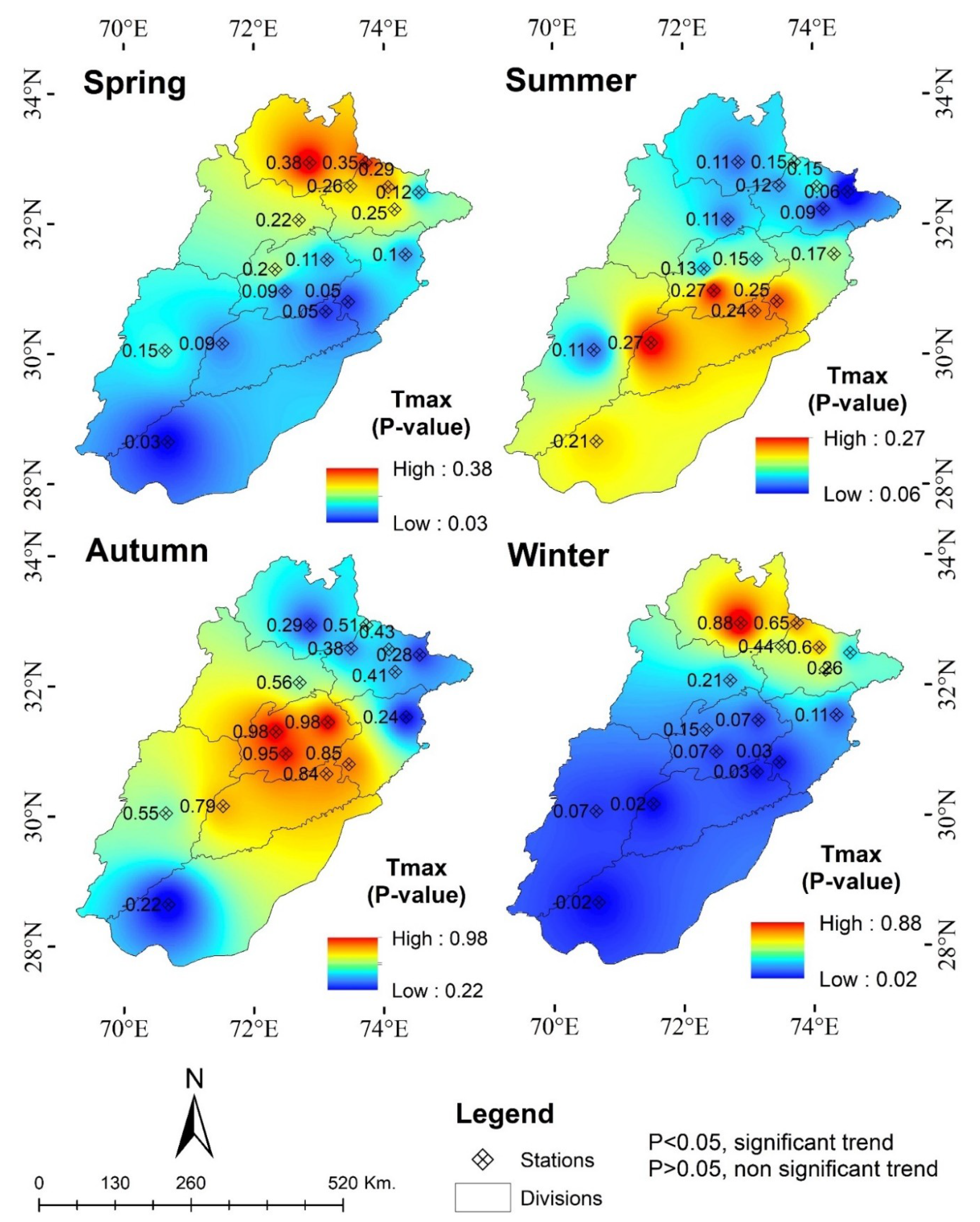
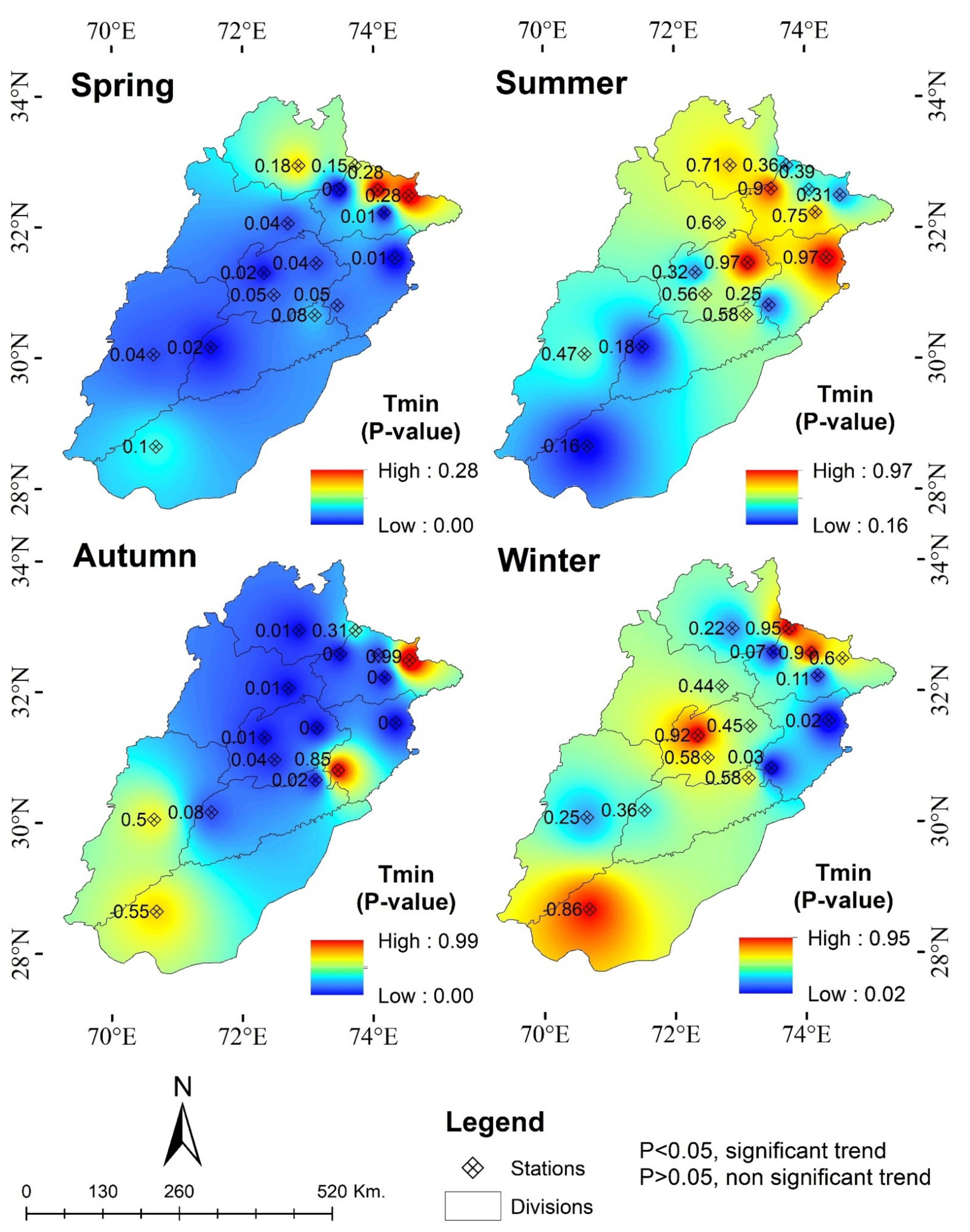
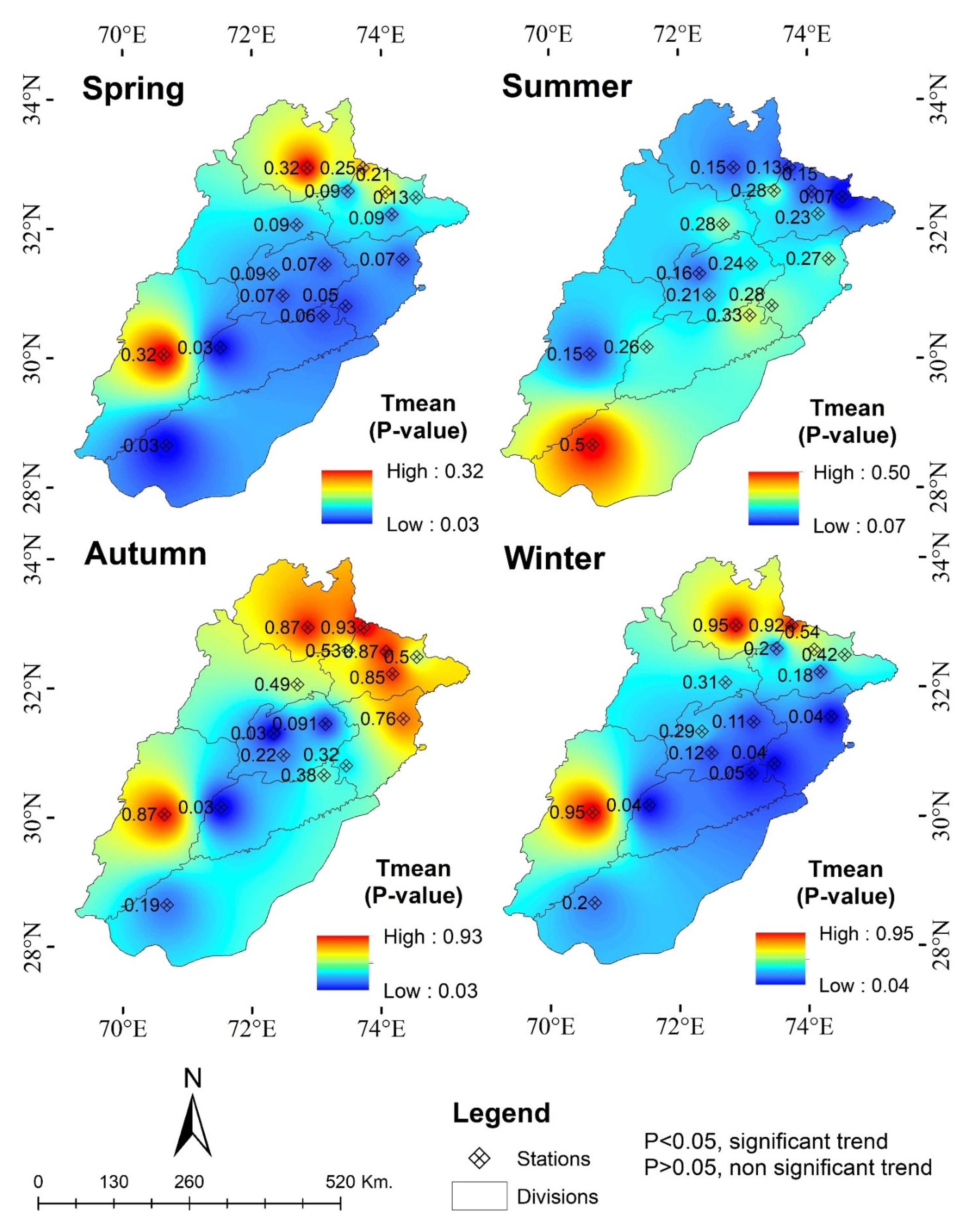
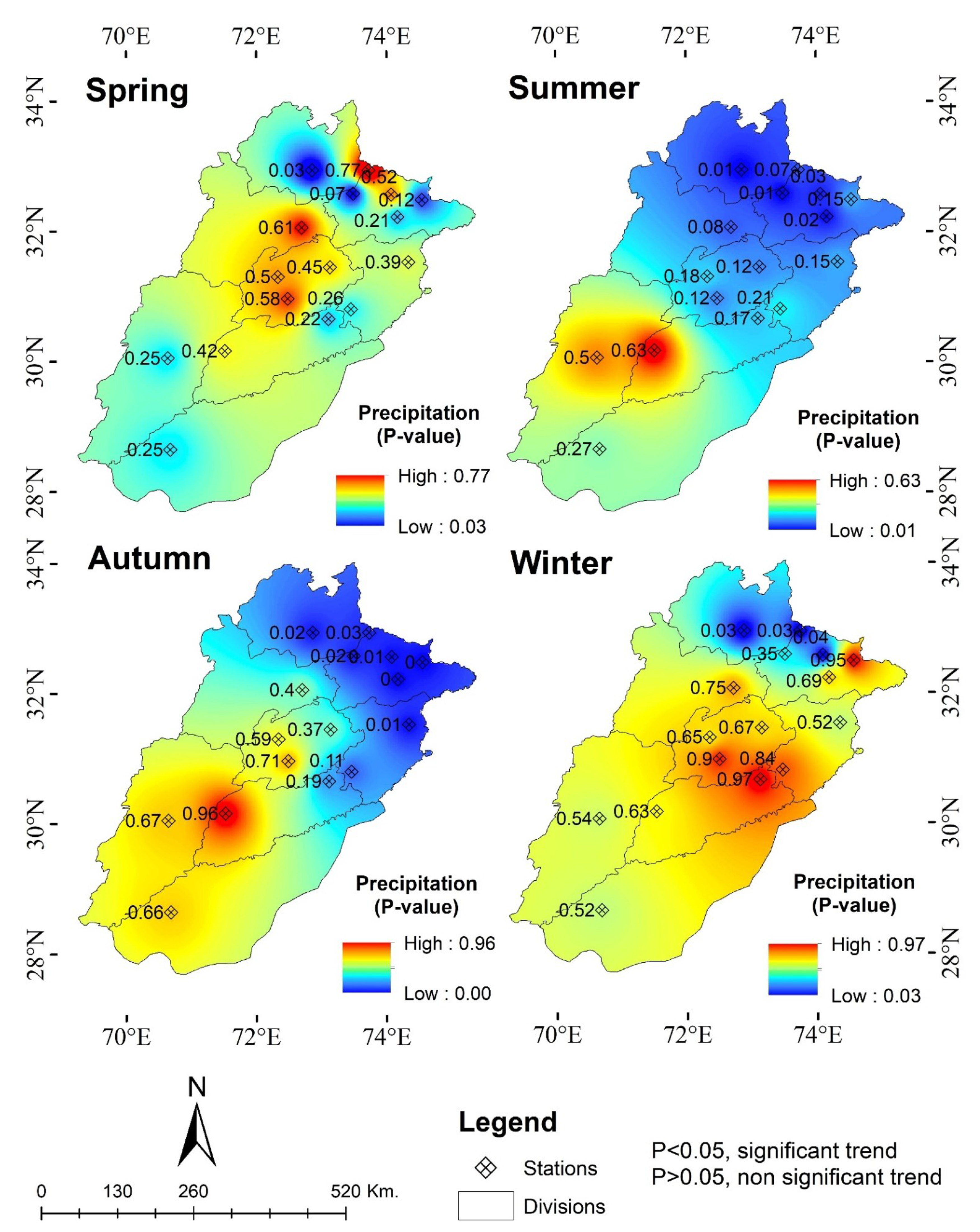
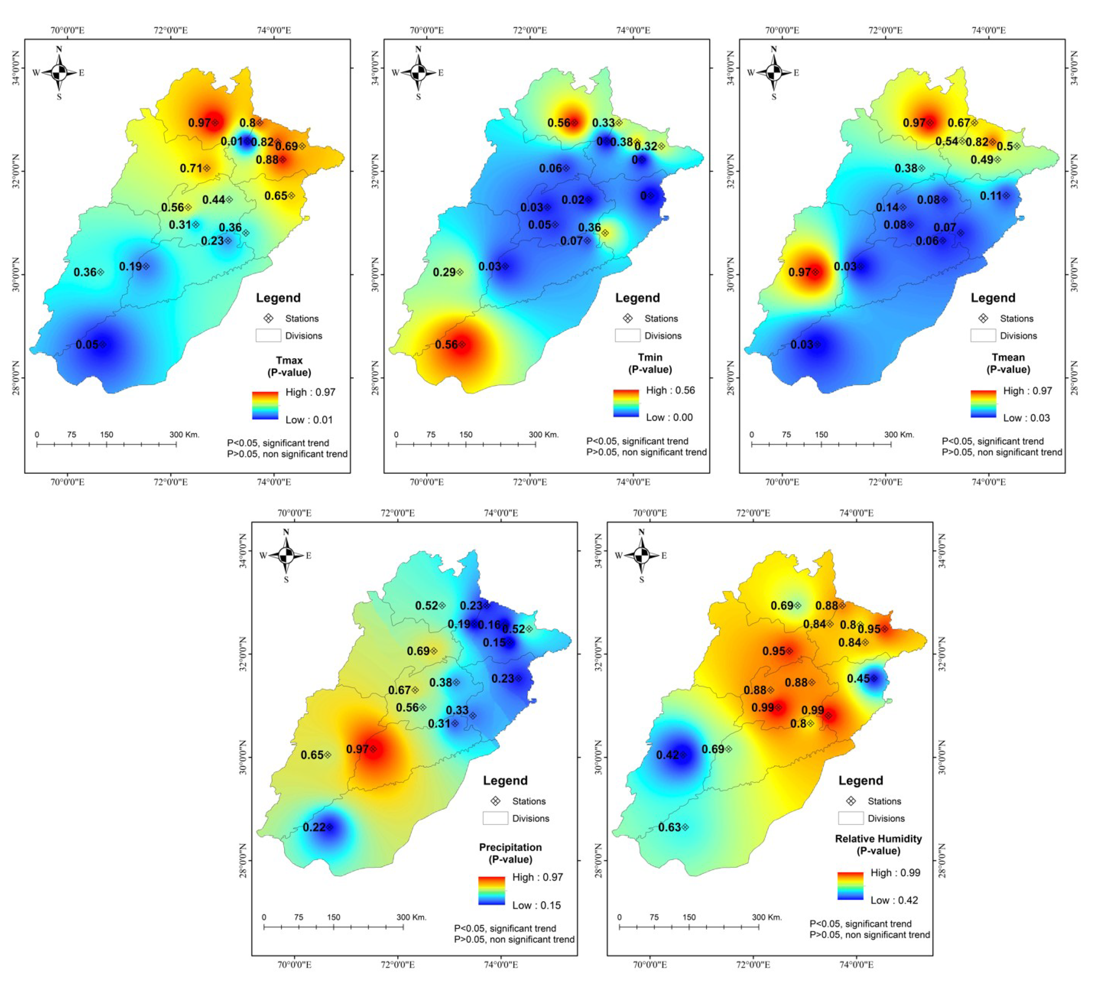
Meanwhile, at the seasonal scale, there was a significant trend shown through SS, which depicted a clear decreasing trend in precipitation in the summer season. The annual and seasonal trends analysis of T_max, T_min, T_mean, precipitation, and relative humidity obtained using the MK, SS, and CS approaches are presented in Table 5 and Table 6. The CS test indicated that all the variables were monotonic. The magnitudes of the statistically significant trends were determined using the MK test and Sen’s slope estimator. These trend analysis tests were applied in two ways. First, they performed by taking the average values of the 16 stations, where results are shown in Table 4, Table 5 and Table 6. Second, the analysis was done for each of the 16 stations separately, where the results are represented in Figure 3, Figure 4, Figure 5, Figure 6, Figure 7 and Figure 8.

5. Discussion

Particularly now, the severe hazards that present high risks to humans and the ecosystems are extreme climatic patterns [77]. Hence, with evidence showing that the severity of extreme climatic patterns has increased since the 1990s, these events are under serious consideration and gaining attention. As part of a time series analysis, the recognition of a monotonic trend has prime importance. For applying statistical methods, a speculative composition requires the detection of trends. Due to the repercussions of climate variability, the non-homogeneity in the trends of hydrological series was shown. Statistical tests assist in identifying trends in stochastic or non-random arrangements. Understanding their potential or size permits us to make an accurate decision regarding already present trends [78]. The data was analyzed through various procedures, which involved performing tests to detect trends, occurrences, and stationarity of the data for the whole Punjab region, the results of which are shown in Table 4. The main concern during trend detection is finding out whether the values of a time series dataset have a familiar fluctuation with the increase of time; to this end, the ADF test aims to evaluate whether the average values or variances of a series change with the time. Almost all analysis techniques must suppose amorphous stationarity in the datasets whether the methods are linear or not. Hence, it is compulsory to check the stationarity using some standard and finite modules. At the same time, the examination of non-stationarity may lead to some awareness of the actual physical implementations.

Consequently, checking whether the datasets are stationary has supreme importance [56]. The result of the stationarity test is given in Table 4. Every single series appeared to be significantly stationary after using the unit root hypothesis of the ADF test. After passing the datasets through the SS, MK, and CS tests, we observed that the power of the CS test was lower in comparison with the MK test for the trends distribution; therefore, the final decision was made based upon the MK test results, which is in line with Rutkowska et al. [78].

The analysis of contemporary past climate data of these stations showed a large variation in precipitation and temperature [8]. T_min presented a significant (p < 0.05) trend, while T_mean presented a non-significant (p > 0.05) trend in spring (MAM). Precipitation manifested a non-significant (p > 0.05) trend in summer (JJA) but a significant (p < 0.05) trend in autumn. Further, the relative humidity showed a non-significant (p > 0.05) trend in the seasonal and annual data. Nonetheless, at the annual scale, no trend was revealed by any of the variables for Punjab, Pakistan.

5.1. Absolute Changes and Trends of Temperature Indices

Punjab, Pakistan, is classified into two regions: (1) southern Punjab, which is an arid region with comparatively high temperatures in the range of 18.5–31.4 °C and a harsh climate, and (2) central Punjab, which is a semi-arid region with a mean temperature in the range of 10.5–24.4 °C and a mild climate [9,79]. Usually, we assume that the main threat of climate variability is to the agriculture of all regions, including arid, semi-arid, and warmer areas worldwide [9,80]. During the past three decades, the increasing temperature was the most crucial factor causing unsustainability [81,82].

In central and southern Punjab, Pakistan, the intensity of severe maximum temperature indices during 1965–2009 was spotted [83,84]. According to [73], during 1997–2002, the highest significant quick variability in the linear trends of temperature was detected for most areas in the Punjab region; as Rahman and Dawood [27] stated, temperature imbalance is the reason for the drought. The country went through a previous and deep-rooted drought during this period, ultimately harming sustainability.

5.1.1. T_max

MK and SS trend tests were used to identify patterns during the study of annual and seasonal temperature variability to determine whether the patterns were increasing, decreasing, or remained unchanged. Depending on the p-value, the null hypothesis of the MK test for trends was accepted or rejected. As per the test results, some of the stations showed no or a low T_max trend over the period 1979–2014. The summer season was rainy and hot. In contrast, the winter was dry and cold [85]. On a seasonal basis, the Khanpur station during spring and the Khanpur, Multan, Okara, and Sahiwal stations during winter displayed significant (p < 0.05) trends during the period 1979–2014 (Table 5 and Table 6). Our findings coincide with the results of Abid et al. [44] in which Khanpur station showed a significant trend in summer (JJA) and winter (DJF) temperature and precipitation during 1980–2013. The annual significant (p < 0.05) trend was only observed by MB Din station for T_max.

Hence, a non-significant (p > 0.05) annual trend was noticed in Chakwal, DG Khan, Faisalabad, Gujranwala, Gujrat, Jhang, Jhelum, Khanpur, Multan, Okara, Sahiwal, Sialkot, TT Singh, and Sargodha. For the summer season, the temperature of Jhelum was extreme [44]. Similarly, in Gujrat and TT Singh, severe T_max and T_min present significant climate-related risks to sustainability, where past trends show a seasonal increase in temperatures. Multan station is in the arid and hottest region of Punjab, with cold winters and sweltering summers. The summer season lasts from May till September, while the winter season starts in December and remains till February. The lowest average temperature in the winter (DJF) season was 4.5 °C, and the highest mean temperature in June was 42.3 °C. On 27 May 2010, a record-breaking temperature of 50 °C was recorded [86]. In response to such weather conditions, variations in summer (MAM) and winter (DJF) seasons swiftly occurred. A non-significant (p > 0.05) trend was shown in the summer season by all stations during 1979–2014. Hussain et al. [87] explained that, in summers, 91% of the farmers stated that the day temperatures were higher than the previous years of this decade; as many as 62.3% reported the same thing for summer nights. Around 36% of farmers said that they found summer nights less hot than days. However, none of the stations showed a significant (p < 0.05) trend in the summer and autumn seasons regarding T_max.

Further, almost 54.2% of them believed that there were more cool days in the winter season, and 42.9% stated the opposite. On the other hand, 19% of the farmers said they found winter days colder than nights, while 79% of respondents noticed less cool days than nights in the winter season. However, few of them observed no change in the past ten years in the winter and summer seasons. Even so, most of the farmers believed that they experienced an instantaneous variability in the climate, which highly affected the agriculture patterns and ultimately lead to the changing sustainability.

5.1.2. T_min

Overall, strengthening the previous studies [73,88], T_min in the spring season showed a significant (p < 0.05) trend. By showing no trend in the summer season, T_min went against [89], where an increasing trend was reported in many areas of Pakistan. According to the MK and SS tests used in the trend analysis for minimum temperature (T_min), Faisalabad, Gujranwala, Jhang, Lahore, MB Din, and Multan, had highly significant (p < 0.05) annual trends. Our results contrast with the findings of Abid et al. [44], who stated that the temperature of Faisalabad station presented significant (p < 0.05) trends in summer (JJA) and winter (DJF) during 1980–2013. We found a non-significant (p > 0.05) trend in Faisalabad for these seasons.

There was no evident trend for summer at any of the stations during 1979–2014. Further, a significant (p < 0.05) trend was shown for autumn in Chakwal, Faisalabad, Gujranwala, Jhang, Lahore, MB Din, Sahiwal, Sargodha, and TT Singh. In winter, only Lahore and Okara manifested significant (p < 0.05) T_min trends.

5.1.3. T_mean

T_mean is the difference between T_max and T_min; it shows how the trends influence each other, either similarly or oppositely. From 1951 to 2000, remarkable variations in T_mean and its frequency in Punjab, Pakistan, were observed [83,84]. According to the predictions of many global circulation models (GCMs) compared with historical measurements, warming will be enhanced in Punjab in the future [8,42]. By the end of this century, an approximately 2–4 °C increase in the T_mean of Punjab is predicted [28,90]. In the current study, by using the MK and SS tests, the most significant trends were found in the Multan region. Highly significant annual, spring, autumn, and winter trends were found over the period, but no trend was found for summer. Some of the stations, namely, Chakwal, DG Khan, Faisalabad, Gujranwala, Gujrat, Jhelum, MB Din, Sargodha, Sialkot, and TT Singh, did not show any significant trend, annually or seasonally. The remaining stations experiences slight trends over the duration. The annual and spring measurements of the Khanpur and Multan stations showed a significant (p < 0.05) trend for Tmean. Jhang and Multan in autumn and Lahore, Multan, Okara, and Sahiwal in winter displayed significant (p < 0.05) trends. The increase in temperature of 2–3 °C in Gujrat, Sialkot, Jhelum, Gujranwala, and Chakwal showed a clear demonstration of warming in the climate [8,91].

5.2. Absolute Changes and Trends in Precipitation

The annual results and trends in precipitation of Punjab, Pakistan, are shown in Figure 8. Within a 95 % confidence interval, the SS and MK test results specified variability in the trends in precipitation on annual and seasonal timescales during 1979–2014. As discussed earlier, no trends were found for annual precipitation in Punjab, Pakistan, using any method, which contradicted the study of [41], who reported a decreasing trend in annual precipitation in this region. Regarding station-specific data, a highly significant (p < 0.05) trend in all four seasons was detected in the Chakwal station, as shown in Figure 6. Other than that, some of the stations, namely, DG Khan, Faisalabad, Jhang, Khanpur, Multan, Okara, Sahiwal, Sargodha, and TT Singh, did not show any seasonal or annual significant trends over the period.

Gujrat presented a significant (p < 0.05) trend for winter (DJF) and summer (JJA), which agreed with the findings of [37], who demonstrated a declining tendency in precipitation in several locations of Pakistan. Gujrat is a partially rain-fed region and mostly relies on precipitation and resources from groundwater for the production of agriculture. Its climate is modest. The mean annual precipitation ranges from 697 to 1401 mm. The main crops of this area are sugarcane, rice, and wheat. The past trends show a tremendous decrease in the precipitation in Gujrat, due to which, the agriculture productivity was highly affected and still under a significant risk [43,92]. The study of Abid et al. [44] stated that, during 1980–2013, Jhelum station experienced a decreasing trend in summer (JJA) precipitation, while Faisalabad showed a decreasing trend in winter (DJF) precipitation. These results are the same as the results of the current study, which showed a non-significant (p > 0.05) trend in these seasons regarding precipitation in Faisalabad.

The basis of risk mapping is the variability in precipitation patterns, and it has an essential role in climate change monitoring [69]. Northern Punjab has average precipitation between 300 and 600 mm, and southern Punjab has average precipitation between 75 and 200 mm [9,79]. The summer weather is hot and somewhat rainy, while the winter season is dry and cold. Because of the monsoons’ influence on climatic events, 60–65% of precipitation is concentrated from May to September [85]. This type of behavior was due to extreme precipitation patterns and indicates that uneven atmospheric events are a reason for the climate variability over the past few years [93].

Usually, northern Punjab has a high precipitation ratio, which decreases when moving toward southern Punjab. The spatial dispersion of cloud cover is the reason for variations in the precipitation across Punjab, Pakistan. The cloud cover is thicker in the north compared with the south. Due to dense precipitation, the north is cooler than the south. The covering of clouds is more extensive, in monsoon and post-monsoon seasons, which sometimes leads to heavy precipitation in the winter season in the north of Punjab, Pakistan. There is more precipitation in the eastern part of Punjab compared to the west.

Precipitation patterns were affected by the elevation above mean sea level. Because of its northern location and subhumid climate, as well as carrying low amounts of precipitation and having high temperatures, Rawalpindi received more precipitation than the other cities. Multan, like the other cities in the study region, received less precipitation due to its southern location and arid climate. In agreement with [41], we found that for Multan, Bahawalnagar, Faisalabad, Sargodha, and Rawalpindi, the wettest years were 2010, 1992, 1997, 2005, and 2007, whereas the driest years were 2002, 1985, 1999, 1987, and 2002. The year 1999 was the driest year, mainly because of no precipitation during autumn in the southern region of Punjab. Along with this, the spring season of 2000 observed no precipitation. This leads to the conclusion that there was no temporal trend in precipitation, but spatial patterns were evident regarding the mean annual precipitation under the impact of elevation above the mean sea level. Same as the study of [73], our findings also found that the majority of the winter precipitation was driven by western disturbances, which resulted in decreased precipitation at most sites in the study region.

5.3. Annual and Seasonal Trends in Relative Humidity

For determining the distribution and occurrence of clouds, an important factor is relative humidity [94]. Patterns of relative humidity are related to the roles of the other analyzed climatic variables. Relative humidity has a direct relation with precipitation but an inverse relation with temperature. A decrease in precipitation also causes a reduction in the relative humidity and the temperature will increase [95]. Changes in relative humidity in the atmosphere are very impactful if the atmospheric relative humidity is interconnected to the precipitation and the surface energy exchanges. To realize the current variability in climate and the prediction for future climate changes, the changes in relative humidity and the assessment of moisture amounts are necessary for estimating the availability of water content and precipitation rate in the atmosphere [96].

In light of Kousari and Zarch’s [97] research results, during recent years, a significant decrease in average yearly relative humidity and a close connection between relative humidity and air temperature were found. We also identified a similar decreasing trend in relative humidity, specifically in the summer season. Other than that, no significant trend was found, seasonally or annually, over Punjab within the timescale 1979–2014. The MK test also showed the same Tau values but in the opposite direction for the maximum temperature and relative humidity in the summer (Table 6). No significant trend was found either annually or for spring or autumn regarding relative humidity, as represented in Figure 7. However, in the summer season, some stations, namely, Chakwal, Faisalabad, Gujranwala, Gujrat, Jhang, Lahore, MB Din, Sargodha, and Sialkot, presented significant (p < 0.05) trends for relative humidity. In winter, DG Khan, Sahiwal, Sargodha, and TT Singh showed significant (p < 0.05) trends.

Contrarily, Khanpur, Multan, and Okara presented non-significant (p > 0.05) trends, both annually and seasonally. All the stations presented non-significant (p > 0.05) trends in spring and autumn regarding relative humidity (Figure 7). A decreasing trend in humidity has a negative influence on the environment [98]. Figure 8 provides the explanation of the station-specific annual time series and the trends for all studied variables for Punjab, Pakistan, during 1979–2014.

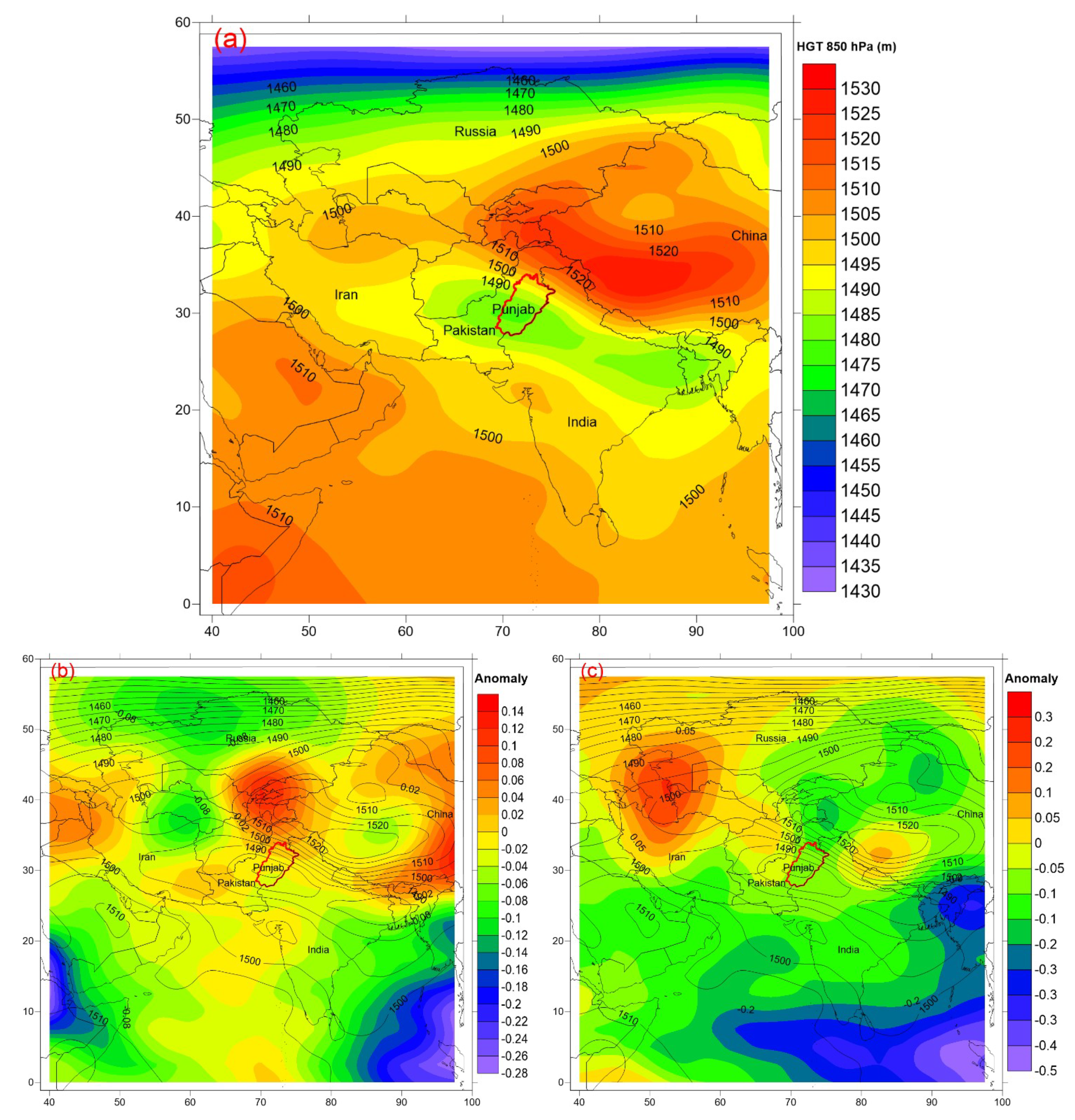
Figure 9a shows the average of the 850 hPa geopotential height (HGT) of the study area during 1979–2014. The figure indicates that, generally, there were two areas with high and low pressure affecting the climate of Punjab. The two areas were (1) the Tibetan high pressure (THP) that was located on the Tibet plateau and (2) a low pressure that was located in the Bay of Bengal (BBLP) to the southeast of Iran. Changes in these two pressure centers were responsible for all climatic phenomena in the study area. Further, there were two centers for each of the two mentioned pressure patterns: the western center of the THP located in northern Punjab and the other western center of BBLP located in the study area. The result of separately studying the dry and wet periods based on seasonal precipitation of each station (≤±2 std for precipitation) during 1979–2014 showed that there were two periods 1999–2002 and 2011–2014 that were found to be very dry and very wet years, respectively, in the study area (Figure 9a). A wet/dry period was defined as having at least 50 percent of the studied stations (i.e., at least eight stations) experiencing higher/lower than average precipitation. This situation continued for at least three seasons.

The changes in the HGT patterns for these two periods showed that a dry period (1999–2002) happened when there was a higher than usual HGT for the western center of THP and a lower than normal HGT for the eastern center of the THP. In this situation, the strengthened western center of the THP extended southward and covered the study area. Because of the high-pressure systems that make a stable climate condition, stopping air mass from ascending, they result in a clear sky [99,100]; therefore, this produces a condition with higher-than-normal temperature and lower-than-normal precipitation and humidity (Figure 9b). A wet period (2011–2014) happened when there was a higher-than-normal HGT for the eastern center of the THP and a lower-than-normal HGT for the western center of the THP. In this situation, the weakened western center of the THP shrunk northward and did not cover the study area; as such, the study area was affected by low pressure and, because of the nature of low-pressure systems, this produced an unstable climate condition, letting air mass ascend, and resulting in a cloudy sky [97]. This produced conditions with lower-than-normal temperature and higher-than-normal precipitation and humidity (Figure 9c).

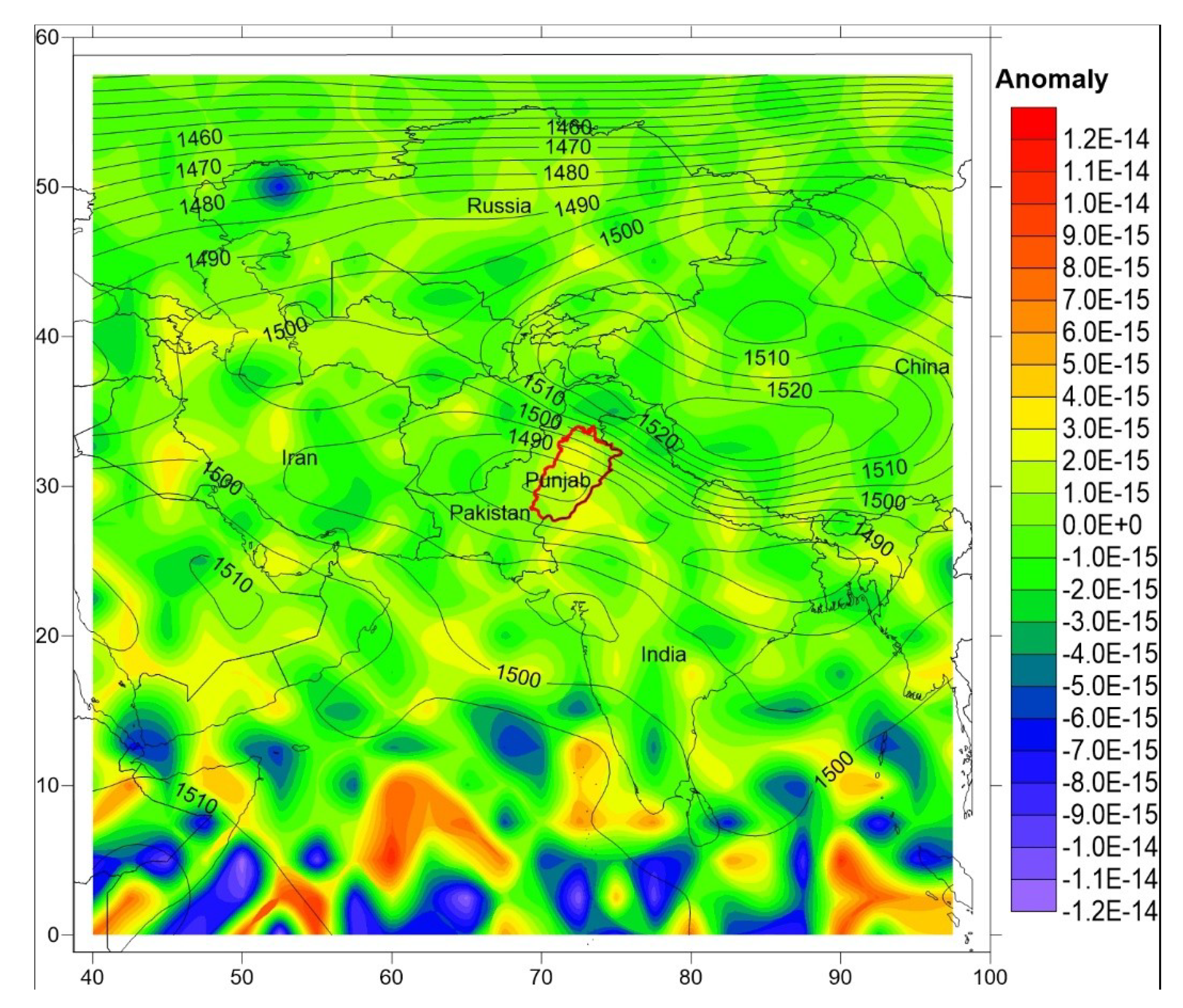
Figure 10 shows the anomaly of the 850 hPa HGT during 1979–2014. The figure indicates that both centers of the THP and BBLP were weaker during the study period. Therefore, it seems that despite having a weaker THP, especially in its western center, because of a weaker THP in the eastern part, the BBLP could move to a higher latitude, and it could have a negative impact on precipitation in Punjab in the future. This situation can have the same impact on all the areas located between 20 and 30° N from India to Pakistan, Afghanistan, and southeastern Iran (Figure 10).

5.4. Comparison of Trends

Further studies [101,102] described a review of the increasing water shortages in arid (e.g., MB Din) and semi-arid regions (mostly TT Singh) because of the increasing risks related to climate variability. Only a few researchers have identified positive changes in the precipitation and temperature in Punjab, Pakistan [103]. According to all methods (Table 5 and Table 6), there were no significant trends in the annual (T_max, T_min, T_mean, precipitation, and relative humidity) time series for Punjab province over the period 1979–2014. Referring to the MK test (Table 6), extremely significant (p < 0.05) trends were noticed for T_min in spring and autumn and for precipitation in autumn. Within a 95% confidence level, the SS results were very similar to the MK results. In the station-specific analyses, the results for two vulnerable stations are presented in

Table 7. MK test results for MB Din for the period 1979–2014.

Variable	Period	Z Statistic	p-Value	Tau	Sen’s Slope
Precipitation	Annual	1.3212	0.1864	0.155556	5.990059
	Spring	−1.7843	0.07437	−0.20952	−1.986163
	Summer	2.4381	0.01476 *	0.285714	6.888515
	Autumn	2.3703	0.01778 *	0.277999	2.180419
	Winter	−0.93984	0.3473	−0.11111	−1.119856
Relative Humidity	Annual	0.20431	0.8381	0.0254	0.000248441
	Spring	−0.83087	0.406	−0.09841	−0.001344464
	Summer	2.2474	0.02461 *	0.263492	0.00381155
	Autumn	1.3895	0.1647	0.163622	0.002674025
	Winter	−1.7299	0.08366	−0.20317	−0.002960556
Tmax	Annual	0.013621	0.013621 *	0.00317	0.001644908
	Spring	1.1305	0.2583	0.133333	0.0560698
	Summer	−1.5664	0.1173	−0.18413	−0.05785319
	Autumn	−0.87182	0.3833	−0.10326	−0.03230826
	Winter	0.77639	0.4375	0.0921	0.01847129
Tmin	Annual	3.6368	0.000276 *	0.425397	0.02845178
	Spring	2.8195	0.004809 *	0.330159	0.0377603
	Summer	0.12259	0.9024	0.0159	0.001404296
	Autumn	3.8142	0.000137 *	0.446386	0.06058493
	Winter	1.7843	0.07437	0.209524	0.02160051
Tmean	Annual	0.61294	0.5399	0.0730	0.008112258
	Spring	1.6754	0.09386	0.196825	0.04790999
	Summer	−1.0761	0.2819	−0.12698	−0.02465581
	Autumn	0.62662	0.5309	0.0747	0.006903813
	Winter	1.294	0.1957	0.152381	0.01773802

(The asterisk “*” sign represents the presence of a significant trend in the datasets).

and

Table 8. MK test results for TT Singh for the period 1979–2014.

Variable	Period	Z Statistic	p-Value	Tau	Sen’s Slope
Precipitation	Annual	0.5857	0.5581	0.0698	0.7988654
	Spring	−0.55846	0.5765	−0.06667	−0.2135985
	Summer	1.5664	0.1173	0.184127	1.015149
	Autumn	0.36776	0.713	0.0444	0.06515984
	Winter	−0.12259	0.9024	−0.01587	−0.01869019
Relative Humidity	Annual	−0.013621	0.9891	−0.00317	−7.18 × 10−6
	Spring	−0.61294	0.5399	−0.07302	−0.000677379
	Summer	1.7843	0.07437	0.209524	0.001419451
	Autumn	1.6209	0.105	0.190476	0.001695443
	Winter	−2.084	0.03716 *	−0.24444	−0.001665935
Tmax	Annual	1.0216	0.307	0.120635	0.01315947
	Spring	1.6754	0.09386	0.196825	0.05313781
	Summer	−1.1033	0.2699	−0.13016	−0.01940146
	Autumn	0.068104	0.9457	0.00952	0.002871189
	Winter	1.7843	0.07437	0.209524	0.03589588
Tmin	Annual	1.975	0.04826 *	0.231746	0.01252046
	Spring	1.9205	0.05479	0.225397	0.02922167
	Summer	−0.5857	0.5581	−0.06984	−0.00636988
	Autumn	2.084	0.03716 *	0.244444	0.02800059
	Winter	0.55846	0.5765	0.0667	0.004580776
Tmean	Annual	1.7299	0.08366	0.203175	0.01432999
	Spring	1.8388	0.06594	0.215873	0.03954732
	Summer	−1.2395	0.2152	−0.14603	−0.01469914
	Autumn	1.2395	0.2152	0.146032	0.0121481
	Winter	1.5664	0.1173	0.184127	0.02027609

(The asterisk “*” sign represents the presence of a significant trend in the datasets).

. MB Din displayed a highly significant (p < 0.05) trend and TT Singh displayed the most non-significant (p > 0.05) trend. Just like the results of Shirazi et al. [104], we found a significant (p < 0.05) trend in the summer and autumn precipitation in MB Din. Relative humidity at this station showed a significant (p < 0.05) trend in summer. Annually significant (p < 0.05) trends were observed for T_max and T_min at this station. T_mean presented non-significant (p > 0.05) trends, both annually and seasonally.

All the stations have been discussed appropriately, but a highly significant trend at α = 0.05 was revealed by MB Din and TT Singh, which show them to be the most vulnerable, as is evident in Table 7 and Table 8. MB Din is situated in central Punjab, Pakistan; therefore, it is likely to show fluctuations in climate. TT Singh is situated in a mixed cropping zone, it covers 3252 km², and it is in the major irrigated zone. There are extreme hot (in summer (JJA)) and cold (in winter (DJF)) climate events that occur in these areas [43]. In TT Singh, the seasonal precipitation showed a historical decreasing trend [44].

However, if we describe each zone individually, there are notable differences. In MB Din, T_max showed a significant annual trend. Regarding the seasonal evaluation, relative humidity in winter (DJF) showed a significant (p < 0.05) trend. The annual and autumn T_min showed a significant (p < 0.05) trend. We discerned a fluctuating pattern in the precipitation in some years, for example, autumn of 1999 and spring of 2000 were dry seasons with zero precipitation in TT Singh. T_max and T_mean showed non-significant (p < 0.05) trends at this station.

6. Climate Variability and Sustainability

Sustainability is a major area of interest in both developed and developing countries, but the recent threat to sustainability can be substantially more critical in developing countries (Pakistan) than they are in developed countries. The main parameters are temperature and precipitation. This research aimed to weigh up current and future climate change and related challenges in Punjab, Pakistan, by considering proposed solutions for sustainability. Despite recognizing the specific variables that can cause the changes in climate across Punjab, Pakistan, our aim was not only to identify the critical indicators that capture climatic instability but also to suggest measures to build a sustainable environment. In this regard, the aim was to directly take part in the efforts that help build a sustainable environment for Punjab, Pakistan. According to the trends, the changes in variables will result in impacts that will contribute negatively to sustainability. The current variability in climate directly negatively affects sustainability and thus also influences the upcoming scenarios. Previous studies described that sustainability indicators were affected by historical climate conditions [105]. MacDonald [106] claimed that higher temperatures, earlier spring warming, and decreased precipitation contributed to the increased environmental imbalance, unsustainability, and drought. Our study contributed the same way. We found precipitation variability and a rise in temperature in the Punjab region. A recent study by Ali et al. [107] found that the main Punjab regions (Bahawalpur, Faisalabad, Mianwali, Multan, Sargodha, and Rahim Yar Khan) were affected by extreme flooding and drought events. Due to warming and the above-explained scenarios, Punjab is facing an alarming situation regarding sustainability. The Punjab region, especially Lahore, is going through the deadliest smog cover in the winter season for the past 5 years.

One of the climate change consequences is drought. At the same time, this occurs gradually over a relatively long period; it affects not only agriculture [108,109] and water resources but also the social and economic sectors. This natural event occurs in almost all climatic regions, although its characteristics fluctuate. The main consequences of climate change, which is caused by increasing greenhouse gas concentrations (especially carbon dioxide) in the atmosphere, are changes in various factors ranging from global temperature, solar radiation absorption, precipitation characteristics, humidity, wind speed, runoff, and sea level to water resources, energy, wildlife, and ecosystems [93,110]. The direct connection between climate change and sustainability was stated in the current research. It will possibly assist the upcoming new ideas and allow for farmers to intensify their systems and techniques, both individually and collectively, toward changing the environment and adaptability consistently regarding all aspects of sustainability.

Urbanization has been increasing in Punjab province for the past few decades. Because it is richer in industrialization than other provinces and has many educational and employment opportunities [111], the people prefer to move to Punjab. The rate of urbanization in Punjab is 36.71 percent [112]. According to the 2017 census, Pakistan’s total population is 207.77 million and the distribution is as follows: 30.52 million in Khyber Pakhtunkhwa (KPK), 5 million in Federally Administered Tribal Area (FATA), 47.89 million in Sindh, 12.34 million in Baluchistan, and 2 million in Islamabad. A major portion of the population that accounts for 110.01 million people is in Punjab province, which is approximately 52.95 percent of Pakistan’s population [1]. This swiftly growing population; the lack of a productive and arranged public transport system, resources, and facilities; and the rapidly increasing rate of personally owned vehicles have an inauspicious effect on the sustainable environment of Punjab. According to the Punjab Development Statistics, 2017, there are 16907529 registered motor vehicles in Punjab, where 79.39 percent are privately owned motorbikes and scooters, and 11.58 percent are personal cars [106]. The prime method of urban transportation of this province is via cars, motorbikes, particularized buses, vans, and qingqi. All of these collectively are substantially affecting the sustainability and climate of Punjab through producing a large volume of smoke through the combustion of fossil fuels [113]. According to a study by Stroik et al. [114], without taking into account natural disasters, anthropogenic emissions accounted for more than half of the average global surface temperature rise between 1951 and 2010. As per EDGAR statistics [115], there was a 169% increase in emissions created by industrial operations, from 17,098 to 46,122 Gg. Most of the CO₂ is produced by industrial processes and procedures, widespread vehicle use, and power generation, whereas methane (CH₄) is produced by poor waste management, conventional agricultural operations, and fossil fuel combustion [116]. Hussain et al. [117] explained how industrialization and urbanization increased the temperature by increasing GHG emissions and accounts for up to 80% of the CO₂ production in Punjab, Pakistan. Defending the work of [118,119,120], alteration in land use patterns caused by anthropogenic operations increase CO₂ emissions to the atmosphere, causing temperatures to rise. The study of [119] demonstrated that variations in land use events, vegetation cover, and deforestation were the principal causes of climate change. Consequently, air pollution is rising expeditiously in Punjab and is documented to be on 195.71 million tons of carbon dioxide (CO₂) emissions annually, which is affecting human health and the sustainable environment [121].

The reported 3590 different kinds of industries in Punjab, Pakistan, also contributing a great part in polluting the environment. In the study of Ghous et al. [122], in the period from 1981 to 2013, a change in temperature due to the increasing pollution in Punjab was found to be 0.021 °C/year. Furthermore, precipitation decreased at an average rate of 0.09 mm/year. Their findings declared that the anthropogenic activities influenced the climate of Lahore, a city of Punjab. Moreover, they revealed that this change will lead to altering the future climate too, which we have explained in our study. Van de Vliert et al. [123] illustrated the mean temperature showed an increasing trend during the period 1961–2010 in all districts of Punjab, Pakistan. However, in this study, the most significant trends were shown by the Multan station during 1979–2014. Due to this fluctuation in temperature, the climate changed quickly, and drastic climate patterns happened more regularly during these years in Punjab, Pakistan. This higher temperature is becoming the cause of extreme events, such as floods and droughts [123]. As the global temperature has been rising over the recent decade and has increased the effects of climate change [124], the Earth’s atmosphere has reached a threshold value, resulting in a combination of moderate and smooth climate change, such as rapid cooling, drying, and warming. Moreover, deforestation is reducing transpiration, which leads to less cloud formation, less rainfall, and enhanced dryness [120]. Correspondingly, anthropogenic activities became a significant contributor to droughts and floods [125].

7. Conclusions

The current study inspected the spatio-temporal heterogeneity of temperature parameters, namely, temperature (T_max, T_min, and T_mean), precipitation, and relative humidity, both seasonally and annually, by using 36 years (1979–2014) of CSFR data from 16 stations placed around Punjab, Pakistan. The trends analyses were also undertaken for Punjab, Pakistan, as a whole. The major summary of this research is explained below:

• Seasonally, warming was more noticeable during the spring, with no or less precipitation. A significant (p < 0.05) trend was noticed for T_min in spring and autumn in Punjab. Autumn precipitation also showed a significant (p < 0.05) trend in Punjab during 1979–2014.
• Annually, no significant trend was found for any of the variables studied, namely, T_max, T_min, T_mean, precipitation, and relative humidity, in the Punjab province.
• Based on station-specific analyses, none of the stations showed a significant (p < 0.05) trend for annual precipitation or annual relative humidity. Similarly, all the stations showed non-significant (p > 0.05) trends for summer T_max, T_min, and T_mean.
• The prime focus of using the CS test was to analyze the monotonic tendency of the variables and the results showed all the variables were monotonic.
• After analyzing the station-specific data, many stations showed significant trends, but the most vulnerable were MB Din and TT Singh.
• The fluctuations in the HGT patterns were the root cause of the changing climate of Punjab, Pakistan, in many ways. In particular, we found that Punjab faced two drastic periods in recent years. One was a wet period, and the other was a dry period. The dry period (1999–2002) resulted in higher temperatures and low precipitation and humidity. In contrast, the wet period (2011–2014) was accompanied by low temperatures and high precipitation and humidity.
• Furthermore, the impact of anthropogenic activities on the variables that are associated with climate dynamics may be an interesting broad research topic that can be studied in the near future.
• To summarize, for the testing of our observations, more work is required. So far, our work covers a combination of assessments that focus on spatial and temporal heterogeneity, thresholds, and climate variability.

References

1. Easterling, D.R.; Evans, J.L.; Groisman, P.Y.; Karl, T.R.; Kunkel, K.E.; Ambenje, P. Observed variability and trends in extreme climate events: A brief review. Bull. Am. Meteorol. Soc. 2000, 81, 417–426. [Google Scholar] [CrossRef] [Green Version]
2. Tabari, H.; Somee, B.S.; Zadeh, M.R. Testing for long-term trends in climatic variables in Iran. Atmos. Res. 2011, 100, 132–140. [Google Scholar] [CrossRef]
3. Stocker, T.F.; Qin, D.; Plattner, G.-K.; Tignor, M.M.; Allen, S.K.; Boschung, J.; Nauels, A.; Xia, Y.; Bex, V.; Midgley, P.M. Climate Change 2013: The Physical Science Basis Contribution of Working Group I to the Fifth Assessment Report of IPCC the Intergovernmental Panel on Climate Change; Cambridge University Press: Cambridge, UK, 2014. [Google Scholar]
4. New, M.; Todd, M.; Hulme, M.; Jones, P. Precipitation measurements and trends in the twentieth century. Int. J. Climatol. 2001, 21, 1889–1922. [Google Scholar] [CrossRef]
5. Jain, S.K.; Kumar, V.; Saharia, M. Analysis of rainfall and temperature trends in northeast India. Int. J. Climatol. 2013, 33, 968–978. [Google Scholar] [CrossRef]
6. Rasul, G.; Mahmood, A.; Sadiq, A.; Khan, S.I. Vulnerability of the Indus delta to climate change in Pakistan. Pak. J. Meteorol. 2012, 8, 89–107. [Google Scholar]
7. Abbas, G.; Ahmad, S.; Ahmad, A.; Nasim, W.; Fatima, Z.; Hussain, S.; Rehman, M.H.; Khan, M.A.; Hasanuzzaman, M.; Fahad, S. Quantification the impacts of climate change and crop management on phenology of maize-based cropping system in Punjab, Pakistan. Agric. For. Meteorol. 2017, 247, 42–55. [Google Scholar] [CrossRef]
8. Bokhari, S.A.A.; Rasul, G.; Ruane, A.C.; Hoogenboom, G.; Ahmad, A. The past and future changes in climate of the rice-wheat cropping zone in Punjab, Pakistan. Pak. J. Meteorol. Vol. 2017, 13, 26. [Google Scholar]
9. Tariq, M.; Ahmad, S.; Fahad, S.; Abbas, G.; Hussain, S.; Fatima, Z.; Nasim, W.; Mubeen, M.; Rehman, M.H.; Khan, M.A. The impact of climate warming and crop management on phenology of sunflower-based cropping systems in Punjab, Pakistan. Agric. For. Meteorol. 2018, 256, 270–282. [Google Scholar] [CrossRef]
10. Chou, C.; Chiang, J.C.; Lan, C.-W.; Chung, C.-H.; Liao, Y.-C.; Lee, C.-J. Increase in the range between wet and dry season precipitation. Nat. Geosci. 2013, 6, 263–267. [Google Scholar] [CrossRef]
11. Jin, M.; Dickinson, R.E. New observational evidence for global warming from satellite. Geophys. Res. Lett. 2002, 29, 39-1–39-4. [Google Scholar] [CrossRef] [Green Version]
12. Shahid, S.; Harun, S.B.; Katimon, A. Changes in diurnal temperature range in Bangladesh during the time period 1961–2008. Atmos. Res. 2012, 118, 260–270. [Google Scholar] [CrossRef]
13. del Río, S.; Anjum Iqbal, M.; Cano-Ortiz, A.; Herrero, L.; Hassan, A.; Penas, A. Recent mean temperature trends in Pakistan and links with teleconnection patterns. Int. J. Climatol. 2013, 33, 277–290. [Google Scholar] [CrossRef]
14. Khan, N.; Shahid, S.; bin Ismail, T.; Wang, X.-J. Spatial distribution of unidirectional trends in temperature and temperature extremes in Pakistan. Theor. Appl. Climatol. 2019, 136, 899–913. [Google Scholar] [CrossRef]
15. Nashwan, M.S.; Shahid, S.; Wang, X. Uncertainty in estimated trends using gridded rainfall data: A case study of Bangladesh. Water 2019, 11, 349. [Google Scholar] [CrossRef] [Green Version]
16. Li, K.; Tong, Z.; Liu, X.; Zhang, J.; Tong, S. Quantitative assessment and driving force analysis of vegetation drought risk to climate change: Methodology and application in Northeast China. Agric. For. Meteorol. 2020, 282, 107865. [Google Scholar] [CrossRef]
17. Kabir, M.H.; Baten, M.A. Sustainability of Climate Change Adaptation Practices in South-Western Coastal Area of Bangladesh. J. Sustain. Dev. 2019, 12, 1–22. [Google Scholar] [CrossRef]
18. Sabziparvar, A.A.; Mir Mousavi, S.H.; Karampour, M.; Doostkamian, M.; Haghighi, E.; Rousta, I.; Olafsson, H.; Sarif, M.O.; Gupta, R.D.; Moniruzzaman, M. Harmonic Analysis of the Spatiotemporal Pattern of Thunderstorms in Iran (1961–2010). Adv. Meteorol. 2019, 2019. [Google Scholar] [CrossRef] [Green Version]
19. Field, C.B.; Barros, V.; Stocker, T.F.; Dahe, Q. Managing the Risks of Extreme Events and Disasters to Advance Climate Change Adaptation: Special Report of the Intergovernmental Panel on Climate Change; Cambridge University Press: Cambridge, UK, 2012. [Google Scholar]
20. Thomas, C.D.; Cameron, A.; Green, R.E.; Bakkenes, M.; Beaumont, L.J.; Collingham, Y.C.; Erasmus, B.F.; De Siqueira, M.F.; Grainger, A.; Hannah, L. Extinction risk from climate change. Nature 2004, 427, 145–148. [Google Scholar] [CrossRef]
21. Malhi, Y.; Roberts, J.T.; Betts, R.A.; Killeen, T.J.; Li, W.; Nobre, C.A. Climate change, deforestation, and the fate of the Amazon. Science 2008, 319, 169–172. [Google Scholar] [CrossRef] [Green Version]
22. Huber, D.G.; Gulledge, J. Extreme Weather and Climate Change: Understanding the Link, Managing the Risk; The Center for Climate and Energy Solutions (C2ES): Arlington, VA, USA, 2011. [Google Scholar]
23. Zhao, J.; Li, K.; Wang, R.; Tong, Z.; Zhang, J. Yield Data Provide New Insight into the Dynamic Evaluation of Maize’s Climate Suitability: A Case Study in Jilin Province, China. Atmosphere 2019, 10, 305. [Google Scholar] [CrossRef] [Green Version]
24. Nashwan, M.S.; Shahid, S.; Chung, E.-S.; Ahmed, K.; Song, Y.H. Development of climate-based index for hydrologic hazard susceptibility. Sustainability 2018, 10, 2182. [Google Scholar] [CrossRef] [Green Version]
25. Ullah, S.; You, Q.; Ullah, W.; Ali, A. Observed changes in precipitation in China-Pakistan economic corridor during 1980–2016. Atmos. Res. 2018, 210, 1–14. [Google Scholar] [CrossRef]
26. Khattak, M.S.; Babel, M.S.; Sharif, M. Hydro-meteorological trends in the upper Indus River basin in Pakistan. Clim. Res. 2011, 46, 103–119. [Google Scholar] [CrossRef]
27. Rahman, G.; Dawood, M. Spatial and temporal variation of rainfall and drought in Khyber Pakhtunkhwa Province of Pakistan during 1971–2015. Arab. J. Geosci. 2018, 11, 46. [Google Scholar] [CrossRef]
28. Ahmad, A.; Ashfaq, M.; Rasul, G.; Wajid, S.A.; Khaliq, T.; Rasul, F.; Saeed, U.; Rahman, M.H.; Hussain, J.; Ahmad Baig, I. Impact of climate change on the rice–wheat cropping system of Pakistan. In Handbook of Climate Change and Agroecosystems: The Agricultural Model Intercomparison and Improvement Project Integrated Crop and Economic Assessments, Part 2; Rosenzweig, C., Hillel, D., Eds.; Imperial College Press: London, UK, 2015; pp. 219–258. [Google Scholar]
29. Reggiani, P.; Mukhopadhyay, B.; Rientjes, T.H.M.; Khan, A. A joint analysis of river runoff and meteorological forcing in the Karakoram, upper Indus Basin. Hydrol. Process. 2017, 31, 409–430. [Google Scholar] [CrossRef]
30. Shirazi, S.A.; Zahid, F.; Bokhari, M.H. Rainfall variability and its impact on some selected crops of Punjab-Pakistan 1973–2003. J. South Asian Stud. 2014, 22, 107–133. [Google Scholar]
31. Dow, K.; Berkhout, F.; Preston, B.L.; Klein, R.J.T.; Midgley, G.; Shaw, M.R. Limits to adaptation. Nat. Clim. Chang. 2013, 3, 305–307. [Google Scholar] [CrossRef]
32. Levin, S.A.; Clark, W. Toward a science of sustainability: Report from toward a science of sustainability conference. CID Work. Pap. Ser. 2010, 196. Available online: https://dash.harvard.edu/bitstream/handle/1/9774654/Clark-TowardScience.pdf?sequence=1&isAllowed=y (accessed on 1 July 2021).
33. Werners, S.E.; Pfenninger, S.; van Slobbe, E.; Haasnoot, M.; Kwakkel, J.H.; Swart, R.J. Thresholds, tipping and turning points for sustainability under climate change. Curr. Opin. Environ. Sustain. 2013, 5, 334–340. [Google Scholar] [CrossRef]
34. Iqbal, M.J.; Ali, M. A probabilistic approach for estimating return period of extreme annual rainfall in different cities of Punjab. Arab. J. Geosci. 2013, 6, 2599–2606. [Google Scholar] [CrossRef]
35. Aslam, A.Q.; Ahmad, I.; Ahmad, S.R.; Hussain, Y.; Hussain, M.S.; Shamshad, J.; Zaidi, S.J.A. Integrated climate change risk assessment and evaluation of adaptation perspective in southern Punjab, Pakistan. Sci. Total Environ. 2018, 628, 1422–1436. [Google Scholar] [CrossRef] [PubMed]
36. Khattak, M.S.; Ali, S. Assessment of temperature and rainfall trends in Punjab province of Pakistan for the period 1961–2014. J. Himal. Earth Sci. 2015, 48, 42. [Google Scholar]
37. Salma, S.; Rehman, S.; Shah, M.A. Rainfall trends in different climate zones of Pakistan. Pak. J. Meteorol. 2012, 9, 37–47. [Google Scholar]
38. Jahangir, M.; Ali, S.M.; Khalid, B. Annual minimum temperature variations in early 21st century in Punjab, Pakistan. J. Atmos. Sol. Terr. Phys. 2016, 137, 1–9. [Google Scholar] [CrossRef]
39. Abbas, F. Analysis of a historical (1981–2010) temperature record of the Punjab province of Pakistan. Earth Interact. 2013, 17, 1–23. [Google Scholar] [CrossRef]
40. Li, L.; Zhang, R.; Wen, M. Structure characteristics of the vortices moving off the Tibetan Plateau. Meteorol. Atmos. Phys. 2020, 132, 19–34. [Google Scholar] [CrossRef]
41. Abbas, F.; Ahmad, A.; Safeeq, M.; Ali, S.; Saleem, F.; Hammad, H.M.; Farhad, W. Changes in precipitation extremes over arid to semiarid and subhumid Punjab, Pakistan. Theor. Appl. Climatol. 2014, 116, 671–680. [Google Scholar] [CrossRef]
42. Amin, A.; Nasim, W.; Mubeen, M.; Sarwar, S.; Urich, P.; Ahmad, A.; Wajid, A.; Khaliq, T.; Rasul, F.; Hammad, H.M. Regional climate assessment of precipitation and temperature in Southern Punjab (Pakistan) using SimCLIM climate model for different temporal scales. Theor. Appl. Climatol. 2018, 131, 121–131. [Google Scholar] [CrossRef]
43. Abid, M.; Scheffran, J.; Schneider, U.A.; Ashfaq, M. Farmers’ perceptions of and adaptation strategies to climate change and their determinants: The case of Punjab province, Pakistan. Earth Syst. Dyn. 2015, 6, 225–243. [Google Scholar] [CrossRef] [Green Version]
44. Abid, M.; Schilling, J.; Scheffran, J.; Zulfiqar, F. Climate change vulnerability, adaptation and risk perceptions at farm level in Punjab, Pakistan. Sci. Total Environ. 2016, 547, 447–460. [Google Scholar] [CrossRef]
45. Hijmans, R.J.; Cameron, S.E.; Parra, J.L.; Jones, P.G.; Jarvis, A. Very high resolution interpolated climate surfaces for global land areas. Int. J. Climatol. 2005, 25, 1965–1978. [Google Scholar] [CrossRef]
46. Samie, A.; Deng, X.; Jia, S.; Chen, D. Scenario-based simulation on dynamics of land-use-land-cover change in Punjab Province, Pakistan. Sustainability 2017, 9, 1285. [Google Scholar] [CrossRef] [Green Version]
47. Didan, K.; Munoz, A.B.; Solano, R.; Huete, A. MODIS Vegetation Index User’s Guide (MOD13 Series). University of Arizona: Vegetation Index and Phenology Lab; Version 3.00 (Collection 6). 2015. Available online: http://vip.arizona.edu/documents/MODIS/MODIS_VI_UsersGuide_June_2015_C6.pdf (accessed on 1 July 2021).
48. Loveland, T.R.; Zhu, Z.; Ohlen, D.O.; Brown, J.F.; Reed, B.C.; Yang, L. An analysis of the IGBP global land-cover characterization process. Photogramm. Eng. Remote Sens. 1999, 65, 1021–1032. [Google Scholar]
49. Fowler, H.J.; Archer, D.R. Conflicting signals of climatic change in the Upper Indus Basin. J. Clim. 2006, 19, 4276–4293. [Google Scholar] [CrossRef] [Green Version]
50. Fedorová, D. Selection of unit root test on the basis of length of the time series and value of ar (1) parameter. Statistika 2016, 96, 3. [Google Scholar]
51. Gilbert, R.O. Statistical Methods for Environmental Pollution Monitoring; John Wiley & Sons: Hoboken, NJ, USA, 1987. [Google Scholar]
52. Jaagus, J. Climatic changes in Estonia during the second half of the 20th century in relationship with changes in large-scale atmospheric circulation. Theor. Appl. Climatol. 2006, 83, 77–88. [Google Scholar] [CrossRef]
53. Cox, D.R.; Stuart, A. Some quick sign tests for trend in location and dispersion. Biometrika 1955, 42, 80–95. [Google Scholar] [CrossRef] [Green Version]
54. Vanya, C.L. Impact of Climate Variability and Change on Sorghum Production in the Lower Shire Valley in Malawi; University of Nairobi: Nairobi, Kenya, 2012. [Google Scholar]
55. Abeysingha, N.S.; Singh, M.; Sehgal, V.K.; Khanna, M.; Pathak, H. Analysis of trends in streamflow and its linkages with rainfall and anthropogenic factors in Gomti River basin of North India. Theor. Appl. Climatol. 2016, 123, 785–799. [Google Scholar] [CrossRef]
56. Wang, W.; Van Gelder, P.H.A.J.M.; Vrijling, J.K. Trend and stationarity analysis for streamflow processes of rivers in western Europe in the 20th century. In Proceedings of the IWA International Conference on Water Economics, Statistics, and Finance, Rethymno, Greece, 8–10 July 2005; pp. 8–10. [Google Scholar]
57. Dickey, D.A.; Fuller, W.A. Distribution of the estimators for autoregressive time series with a unit root. J. Am. Stat. Assoc. 1979, 74, 427–431. [Google Scholar]
58. Said, S.E.; Dickey, D.A. Testing for unit roots in autoregressive-moving average models of unknown order. Biometrika 1984, 71, 599–607. [Google Scholar] [CrossRef]
59. Zamani, R.; Mirabbasi, R.; Abdollahi, S.; Jhajharia, D. Streamflow trend analysis by considering autocorrelation structure, long-term persistence, and Hurst coefficient in a semi-arid region of Iran. Theor. Appl. Climatol. 2017, 129, 33–45. [Google Scholar] [CrossRef]
60. Partal, T. Wavelet transform-based analysis of periodicities and trends of Sakarya basin (Turkey) streamflow data. River Res. Appl. 2010, 26, 695–711. [Google Scholar] [CrossRef]
61. Chen, Y.; Guan, Y.; Shao, G.; Zhang, D. Investigating trends in streamflow and precipitation in Huangfuchuan Basin with wavelet analysis and the Mann-Kendall test. Water 2016, 8, 77. [Google Scholar] [CrossRef] [Green Version]
62. Yue, S.; Wang, C. The Mann-Kendall test modified by effective sample size to detect trend in serially correlated hydrological series. Water Resour. Manag. 2004, 18, 201–218. [Google Scholar] [CrossRef]
63. Koutsoyiannis, D.; Montanari, A. Statistical analysis of hydroclimatic time series: Uncertainty and insights. Water Resour. Res. 2007, 43. [Google Scholar] [CrossRef]
64. Sen, P.K. Estimates of the regression coefficient based on Kendall’s tau. J. Am. Stat. Assoc. 1968, 63, 1379–1389. [Google Scholar] [CrossRef]
65. Militino, A.F.; Moradi, M.; Ugarte, M.D. On the Performances of Trend and Change-Point Detection Methods for Remote Sensing Data. Remote Sens. 2020, 12, 1008. [Google Scholar] [CrossRef] [Green Version]
66. Farnsworth, D.L. A cautionary note concerning the Cox and Stuart test. Teach. Stat. 2001, 23, 76–79. [Google Scholar] [CrossRef]
67. Steinke, V.A.; Martins Palhares de Melo, L.A.; Luiz Melo, M.; Rodrigues da Franca, R.; Luna Lucena, R.; Torres Steinke, E. Trend Analysis of air Temperature in the Federal District of Brazil: 1980–2010. Climate 2020, 8, 89. [Google Scholar] [CrossRef]
68. Conover, W. Practical Nonparametric Statistics, 3rd ed.; John Wiley & Sons: New York, NY, USA, 1999; Volume 578. [Google Scholar]
69. Wang, R.; Zhang, J.; Guo, E.; Zhao, C.; Cao, T. Spatial and temporal variations of precipitation concentration and their relationships with large-scale atmospheric circulations across Northeast China. Atmos. Res. 2019, 222, 62–73. [Google Scholar] [CrossRef]
70. Gupta, A.; Moniruzzaman, M. Spatio-Temporal Analysis of Changing Rainfall Pattern of Bangladesh Using Geo-Spatial Tools. In Proceedings of the International Conference on Weather Forecasting and Advances in Physics (CWFAP), Khulna, Bangladesh, 11–12 May 2018. [Google Scholar]
71. Kisi, O.; Ay, M. Comparison of Mann–Kendall and innovative trend method for water quality parameters of the Kizilirmak River, Turkey. J. Hydrol. 2014, 513, 362–375. [Google Scholar] [CrossRef]
72. Da Silva, R.M.; Santos, C.A.G.; Moreira, M.; Corte-Real, J.; Silva, V.C.; Medeiros, I.C. Rainfall and river flow trends using Mann–Kendall and Sen’s slope estimator statistical tests in the Cobres River basin. Nat. Hazards 2015, 77, 1205–1221. [Google Scholar] [CrossRef]
73. Nawaz, Z.; Li, X.; Chen, Y.; Guo, Y.; Wang, X.; Nawaz, N. Temporal and Spatial Characteristics of Precipitation and Temperature in Punjab, Pakistan. Water 2019, 11, 1916. [Google Scholar] [CrossRef] [Green Version]
74. Iqbal, M.; Wen, J.; Wang, X.; Lan, Y.; Tian, H.; Anjum, M.N.; Adnan, M. Assessment of air temperature trends in the Source Region of Yellow River and its sub-basins, China. Asia-Pac. J. Atmos. Sci. 2018, 54, 111–123. [Google Scholar] [CrossRef]
75. Mitchell, J.M.; Dzerdzeevskii, B.; Flohn, H.; Hofmeyr, W.L.; Lamb, H.H.; Rao, K.N.; Wallén, C.C. Climatic change. Technical Note, No. 79. World Meteorol. Organ. Geneva Switz. 1966, 99, 79. [Google Scholar]
76. Ye, L. Hydrological Mann-Kendal multivariate trends analysis in the Upper Yangtze River basin. J. Geosci. Environ. Prot. 2015, 3, 34. [Google Scholar] [CrossRef]
77. Guo, E.; Zhang, J.; Wang, Y.; Quan, L.; Zhang, R.; Zhang, F.; Zhou, M. Spatiotemporal variations of extreme climate events in Northeast China during 1960–2014. Ecol. Indic. 2019, 96, 669–683. [Google Scholar] [CrossRef]
78. Rutkowska, A. Properties of the Cox–Stuart test for trend in application to hydrological series: The simulation study. Commun. Stat. Simul. Comput. 2015, 44, 565–579. [Google Scholar] [CrossRef]
79. Akram, N.; Hamid, A. Climate change: A threat to the economic growth of Pakistan. Prog. Dev. Stud. 2015, 15, 73–86. [Google Scholar] [CrossRef]
80. Adams, R.M.; Hurd, B.H.; Lenhart, S.; Leary, N. Effects of global climate change on agriculture: An interpretative review. Clim. Res. 1998, 11, 19–30. [Google Scholar] [CrossRef] [Green Version]
81. Liu, Z.; Hubbard, K.G.; Lin, X.; Yang, X. Negative effects of climate warming on maize yield are reversed by the changing of sowing date and cultivar selection in Northeast China. Glob. Chang. Biol. 2013, 19, 3481–3492. [Google Scholar] [CrossRef]
82. Siebert, S.; Ewert, F. Spatio-temporal patterns of phenological development in Germany in relation to temperature and day length. Agric. For. Meteorol. 2012, 152, 44–57. [Google Scholar] [CrossRef]
83. Sheikh, M.M.; Manzoor, N. Region-wise Climate Changes in Pakistan (1951–2000). In Proceedings of the National Workshop on Global Change Perspective in Pakistan, Islamabad, Pakistan, 28–30 April 2005. [Google Scholar]
84. Zahid, M.; Rasul, G. Frequency of extreme temperature and precipitation events in Pakistan 1965–2009. Sci. Int. 2011, 23, 313–319. [Google Scholar]
85. Guna, A.; Zhang, J.; Tong, S.; Bao, Y.; Han, A.; Li, K. Effect of Climate Change on Maize Yield in the Growing Season: A Case Study of the Songliao Plain Maize Belt. Water 2019, 11, 2108. [Google Scholar] [CrossRef] [Green Version]
86. Merlone, A.; Al-Dashti, H.; Faisal, N.; Cerveny, R.S.; AlSarmi, S.; Bessemoulin, P.; Brunet, M.; Driouech, F.; Khalatyan, Y.; Peterson, T.C. Temperature extreme records: World Meteorological Organization metrological and meteorological evaluation of the 54.0 C observations in Mitribah, Kuwait and Turbat, Pakistan in 2016/2017. Int. J. Climatol. 2019, 39, 5154–5169. [Google Scholar] [CrossRef]
87. Hussain, A.; Memon, J.A.; Hanif, S. Weather shocks, coping strategies and farmers’ income: A case of rural areas of district Multan, Punjab. Weather Clim. Extrem. 2020, 30, 100288. [Google Scholar] [CrossRef]
88. Qasim, M.; Khlaid, S.; Shams, D.F. Spatiotemporal variations and trends in minimum and maximum temperatures of Pakistan. J. Appl. Environ. Biol. Sci. 2014, 4, 85–93. [Google Scholar]
89. Ullah, S.; You, Q.; Ali, A.; Ullah, W.; Jan, M.A.; Zhang, Y.; Xie, W.; Xie, X. Observed changes in maximum and minimum temperatures over China-Pakistan economic corridor during 1980–2016. Atmos. Res. 2019, 216, 37–51. [Google Scholar] [CrossRef]
90. Afzaal, M.; Haroon, M.A.; Zaman, Q. Interdecadal oscillations and the warming trend in the area-weighted annual mean temperature of Pakistan. Pak. J. Meteorol. 2009, 6, 13–19. [Google Scholar]
91. Ahmad, I.; Tang, D.; Wang, T.; Wang, M.; Wagan, B. Precipitation trends over time using Mann–Kendall and Spearman’s rho tests in Swat River basin, Pakistan. Adv. Meteorol. 2015, 15, 2015. [Google Scholar] [CrossRef] [Green Version]
92. Ahmad, M.I.; Ma, H. Climate Change and Livelihood Vulnerability in Mixed Crop–Livestock Areas: The Case of Province Punjab, Pakistan. Sustainability 2020, 12, 586. [Google Scholar] [CrossRef] [Green Version]
93. Rousta, I.; Nasserzadeh, M.H.; Jalali, M.; Haghighi, E.; Ólafsson, H.; Ashrafi, S.; Doostkamian, M.; Ghasemi, A. Decadal spatial-temporal variations in the spatial pattern of anomalies of extreme precipitation thresholds (Case Study: Northwest Iran). Atmosphere 2017, 8, 135. [Google Scholar] [CrossRef] [Green Version]
94. Price, J.D.; Wood, R. Comparison of probability density functions for total specific humidity and saturation deficit humidity, and consequences for cloud parametrization. Q. J. R. Meteorol. Soc. A J. Atmos. Sci. Appl. Meteorol. Phys. Oceanogr. 2002, 128, 2059–2072. [Google Scholar] [CrossRef]
95. da Silva, V.d.P.R. On climate variability in Northeast of Brazil. J. Arid. Environ. 2004, 58, 575–596. [Google Scholar] [CrossRef]
96. Xie, B.; Zhang, Q.; Ying, Y. Trends in precipitable water and relative humidity in China: 1979–2005. J. Appl. Meteorol. Climatol. 2011, 50, 1985–1994. [Google Scholar] [CrossRef]
97. Kousari, M.R.; Zarch, M.A.A. Minimum, maximum, and mean annual temperatures, relative humidity, and precipitation trends in arid and semi-arid regions of Iran. Arab. J. Geosci. 2011, 4, 907–914. [Google Scholar] [CrossRef]
98. Neil, K.; Wu, J. Effects of urbanization on plant flowering phenology: A review. Urban Ecosyst. 2006, 9, 243–257. [Google Scholar] [CrossRef]
99. Barry, R.G.; Chorley, R.J. Atmosphere, Weather and Climate; Routledge: London, UK, 2003. [Google Scholar]
100. Nebout, N.C.; Turon, J.; Zahn, R.; Capotondi, L.; Londeix, L.; Pahnke, K. Enhanced aridity and atmospheric high-pressure stability over the western Mediterranean during the North Atlantic cold events of the past 50 ky. Geology 2002, 30, 863–866. [Google Scholar] [CrossRef] [Green Version]
101. Asif, M. Climatic Change, Irrigation Water Crisis and Food Security in Pakistan; Uppsala Universitet: Uppsala, Sweden, 2013. [Google Scholar]
102. Bukhari, M.H.; Sayal, E.A. Emerging climate changes and water resource situation in Pakistan. Pak. Vis. 2011, 12, 236. [Google Scholar]
103. Siddiqui, R.; Samad, G.; Nasir, M.; Jalil, H.H. The impact of climate change on major agricultural crops: Evidence from Punjab, Pakistan. Pak. Dev. Rev. 2012, 51, 261–274. [Google Scholar] [CrossRef] [Green Version]
104. Shirazi, S.; Hussain, M.; Abbas, S.; Lee, S. Climate change impact on agriculture and prevalence of food security in Punjab, Pakistan. Pak. J. Sci. 2020, 72, 230. [Google Scholar]
105. McNeeley, S.M. Sustainable climate change adaptation in Indian country. Weather Clim. Soc. 2017, 9, 393–404. [Google Scholar] [CrossRef]
106. MacDonald, G.M. Water, climate change, and sustainability in the southwest. Proc. Natl. Acad. Sci. USA 2010, 107, 21256–21262. [Google Scholar] [CrossRef] [Green Version]
107. Ali, S.M.; Khalid, B.; Akhter, A.; Islam, A.; Adnan, S. Analyzing the occurrence of floods and droughts in connection with climate change in Punjab province, Pakistan. Nat. Hazards 2020, 103, 2533–2559. [Google Scholar] [CrossRef]
108. Dhakal, S.; Sedhain, G.K.; Dhakal, S.C. Climate change impact and adaptation practices in agriculture: A case study of Rautahat District, Nepal. Climate 2016, 4, 63. [Google Scholar] [CrossRef] [Green Version]
109. Sedhain, G.K.; Dhakal, S.; Dhakal, S.K.; Adhikary, R.K. Effects of changing precipitation patterns on agricultural practices of farmers in Rautahat, Nepal. Res. Briefs. 2016, 75. Available online: http://www.ncckmcnast.org.np/sites/default/files/Research%20Briefs%20Building%20Knowledge%20for%20Climate%20Resilience%20in%20Nepal.pdf#page=89 (accessed on 1 July 2021).
110. Wehbe, M.B.; Seiler, R.A.; Vinocur, M.R.; Eakin, H.; Santos, C.; Civitaresi, H.M. Social Methods for Assessing Agricultural Producers’ Vulnerability to Climate Variability and Change Based on the Notion of Sustainability. Assessments of Impacts and Adaptations of Climate Change Working Papers. 2005. Available online: https://www.semanticscholar.org/paper/Social-Methods-for-Assessing-Agricultural-to-and-on-Vinocur-Eakin/0128bf863878cfbca8e5f5c695eb6f3c473f2507 (accessed on 1 July 2021).
111. Mukhtar, U.; Zhangbao, Z.; Beihai, T.; Naseer, M.; Razzaq, A.; Hina, T. Implications of decreasing farm size on urbanization: A case study of Punjab Pakistan. J. Soc. Sci. Stud. 2018, 5, 71–86. [Google Scholar] [CrossRef] [Green Version]
112. Pakistan Bureau of Statistics. Provisional Province Wise Population by Sex & Rural/Urban of 6th Population & Housing Census of Pakistan; Pakistan Bureau of Statistics: 2017. Available online: https://www.pbs.gov.pk/sites/default/files//Population_Census_2017_Results_0.pdf (accessed on 1 July 2021).
113. Sajjad, S.; Shirazi, S.A.; Khan, M.A.; Raza, A. Urbanization effects on temperature trends of Lahore during 1950–2007. Int. J. Clim. Chang. Strateg. Manag. 2009, 1, 274–281. [Google Scholar] [CrossRef]
114. Stroik, P.; Chakraborty, D.; Ge, W.; Boulter, J.; Jamelske, E. Effect of reciprocity on public opinion of international climate treaties: Experimental evidence from the US and China. Clim. Policy 2019, 19, 959–973. [Google Scholar] [CrossRef]
115. EDGAR; European Commission; Netherlands Environmental Assessment Agency (PBL). Emission Database for Global Atmospheric Research (EDGAR), r.v.; 4.0. 2009. Available online: https://edgar.jrc.ec.europa.eu/ (accessed on 1 July 2021).
116. Zuberi, M.J.S.; Ali, S.F. Greenhouse effect reduction by recovering energy from waste landfills in Pakistan. Renew. Sustain. Energy Rev. 2015, 44, 117–131. [Google Scholar] [CrossRef]
117. Hussain, M.; Butt, A.R.; Uzma, F.; Ahmed, R.; Rehman, A.; Ali, M.U.; Ullah, H.; Yousaf, B. Divisional disparities on climate change adaptation and mitigation in Punjab, Pakistan: Local perceptions, vulnerabilities, and policy implications. Environ. Sci. Pollut. Res. 2019, 26, 31491–31507. [Google Scholar] [CrossRef] [PubMed]
118. Shirazi, S.; Abbas, S.; Khurshid, M.; Shakarullah, K.; Yaseen, M.; Mazhar, N.; Wahla, S. Trends and variability of temperature time series over the kanshi catchment in the potohar region of punjab-pakistan. Pak. J. Sci. 2020, 72, 241–248. [Google Scholar]
119. Copeland, J.; McKelvey, K.; Aubry, K.; Landa, A.; Persson, J.; Inman, R.; Krebs, J.; Lofroth, E.; Golden, H.; Squires, J. The bioclimatic envelope of the wolverine (Gulo gulo): Do climatic constraints limit its geographic distribution? Can. J. Zool. 2010, 88, 233–246. [Google Scholar] [CrossRef]
120. Neupane, M.; Dhakal, S. Climatic Variability and Land Use Change in Kamala Watershed, Sindhuli District, Nepal. Climate 2017, 5, 11. [Google Scholar] [CrossRef] [Green Version]
121. Yaqoob, H.; Teoh, Y.H.; Goraya, T.S.; Sher, F.; Jamil, M.A.; Rashid, T.; Yar, K.A. Energy evaluation and environmental impact assessment of transportation fuels in Pakistan. Case Stud. Chem. Environ. Eng. 2021, 3, 100081. [Google Scholar] [CrossRef]
122. Ghous, M.; Khalida, K.; Basit, A.; Hassan, J. Temporal analysis of urbanization and resulting local weather change: A case study of Lahore, Punjab, Pakistan. Sci. Int. 2015, 27, 1281–1287. [Google Scholar]
123. Van de Vliert, E.; Schwartz, S.H.; Huismans, S.E.; Hofstede, G.; Daan, S. Temperature, cultural masculinity, and domestic political violence: A cross-national study. J. Cross-Cult. Psychol. 1999, 30, 291–314. [Google Scholar] [CrossRef] [Green Version]
124. Cohen, J.L.; Furtado, J.C.; Barlow, M.; Alexeev, V.A.; Cherry, J.E. Asymmetric seasonal temperature trends. Geophys. Res. Lett. 2012, 39. [Google Scholar] [CrossRef]
125. Michaelowa, A. National Research Council, Abrupt Climate Change: Inevitable Surprises. Clim. Chang. 2004, 64, 377–380. [Google Scholar] [CrossRef]
Figure 1. The map of Punjab, Pakistan, showing the districts with 16 CSFR stations.
Atmosphere 12 00939 g001
Figure 2. Land-cover type map of Punjab, Pakistan, that was identified from MODIS (MCD12Q1) images using IGBP classifications.
Atmosphere 12 00939 g002
Figure 3. Seasonal p-values and the trends in Tmax (°C) of the 16 stations of Punjab, Pakistan, over the period 1979–2014.
Atmosphere 12 00939 g003
Figure 4. Seasonal p-values and the trends in Tmin (°C) of the 16 stations of Punjab, Pakistan, over the period 1979–2014.
Atmosphere 12 00939 g004
Figure 5. Seasonal p-values and the trends in Tmean (°C) of the 16 stations of Punjab, Pakistan, over the period 1979–2014.
Atmosphere 12 00939 g005
Figure 6. Seasonal p-values and the trends in precipitation (mm) of the 16 stations of Punjab, Pakistan, over the period 1979–2014.
Atmosphere 12 00939 g006
Figure 7. Seasonal p-values and the trends in relative humidity of the 16 stations of Punjab, Pakistan, over the period 1979–2014.
Atmosphere 12 00939 g007
Figure 8. Annual temporal trends and p-values for Tmax (°C), Tmin (°C), Tmean (°C), precipitation (mm), and relative humidity at the 16 stations of Punjab, Pakistan, over the period 1979–2014.
Atmosphere 12 00939 g008
Figure 9. Average of the 850 hPa HGT during different periods in Punjab, Pakistan: (a) average of the 850 hPa HGT during 1979–2014, (b) average of the 850 hPa HGT during 1979–2014 (contour) and the anomaly of the 850 hPa HGT for the dry period (1999–2003) (shaded), and (c) average of the 850 hPa HGT during 1979–2014 (contour) and the anomaly of the 850 hPa HGT for the wet period (2011–2014) (shaded).
Atmosphere 12 00939 g009
Figure 10. The anomaly of the 850 hPa HGT (shaded) and the mean of the 850 hPa HGT (contour) during 1979–2014.
Atmosphere 12 00939 g010