Abstract
To promote research studies on air pollution and climate change, the mobile laboratory cc-TrAIRer (Climate Change—TRailer for AIR and Environmental Research) was designed and built. It consists of a trailer which affords particles, gas, meteorological and noise measurements. Thanks to its structure and its versatility, it can easily conduct field campaigns in remote areas. The literature review presented in this paper shows the main characteristics of the existing mobile laboratories. The cc-TrAIRer was built by evaluating technical aspects, instrumentations and auxiliary systems that emerged from previous studies in the literature. Some of the studies conducted in heterogeneous topography areas, such as the Po Valley and the Alps, using instruments that were chosen to be located on the mobile laboratory are here reported. The preliminary results highlight the future applications of the trailer and the importance of high temporal resolution data acquisition for the characterization of pollution phenomena. The potential applications of the cc-TrAIRer concern different fields, such as complex terrain, emergency situations, worksite and local source impacts and temporal and spatial distributions of atmospheric compounds. The integrated use of gas and particle analysers, a weather station and environment monitoring systems in a single easily transportable vehicle will contribute to research studies on global aspects of climate change.
1. Introduction
Air quality and atmospheric pollution are still serious challenges worldwide [1,2,3]. Indeed, air pollution contributes to at least 7 million deaths worldwide every year [4,5,6]. According to the State of Global Air 2020 report of the Health Effect Institute, in 2019, it moved up from the fifth to the fourth cause of global deaths, covering 12% of the total.
Atmospheric pollutants can be directly emitted by both anthropogenic and natural sources: although the former are the most significant contributors to the major compounds, the latter should not be overlooked [7,8]. These primary compounds can also chemically interact to promote the formation of secondary air pollutants [9]. Activities related to the combustion of fossil fuels (coal, oil, gas and gasoline), energy production, agricultural burning or other industrial processes for power generation, space heating and transportation significantly increase the particulate matter (PM) concentration in the atmosphere [10,11]. At the same time, fires, sea spray, soil erosion and resuspension of dust naturally contribute to particulate matter increment [12]. Sources of CO include fossil fuels and motor vehicle exhausts, while the burning of coal and oil raises SO2 concentration values [13,14,15]. NOx and VOC are two other critical air pollutants with health and environmental aspects, but they are also involved in the ground-level ozone production mechanism. CO, VOCs and CH4 are, in fact, oxidized in the presence of solar radiation and NOx to form ozone, a secondary pollutant responsible for photochemical smog and health risks linked to respiratory diseases [16,17].
Exposure to high concentrations of gas and particle pollutants gives rise to demonstrated negative effects on the environment and on human health [18,19,20,21]. In adverse conditions of both outdoor and indoor pollution, a large number of organs can generally be affected, such as the lungs [22], heart and brain [23] and eyes [24]. Air pollution also causes relevant impacts on cancers [25], cardiovascular diseases [26], diabetes and obesity [27] and subjective well-being [28]. Air pollutants are also strongly harmful to the environment, with devastating consequences evident. For instance, soil and water matrices are damaged by the effects of acid rains, which usually corrode buildings, statues and infrastructures too [29]. Anthropic emissions, such as those from traffic or industrial activities, contribute to the production of haze, which strongly reduces the atmospheric visibility, especially when opportune accumulation conditions occur [30]. Moreover, the excessive deposition of nitrogen oxides and other nutrients affects the local eutrophication phenomena of surface water and consequently results in damage to aquatic ecosystems [31]. In wider terms, wildlife is dangerously threatened by the effects of air pollution [32].
It is now known that there is a mutual relationship between air pollution and climate change [32]. The compositions of some constituents of PM, such as black carbon, can induce a warming effect on the overall climate through the absorption of solar and infrared radiation [33]. Furthermore, the deposition of these particles on the surfaces of glaciers promotes their melting [34]. Since particles are actively involved in cloud formation, their atmospheric concentration can affect the cloud reflection of solar radiation, the temporal and physical characteristics of precipitations and how long they last [2]. Simultaneously, the main, direct consequences of climate change, such as the warming over the higher latitude areas and the decrease in the frequencies of cyclones, influence the air pollution phenomena [35]. Indeed, the alteration of meteorological events and atmospheric stability directly affects the concentration of PM and ozone [35,36]. The reduction of the number of precipitation and wind events increases the stagnation conditions and decreases the possibility of the dilution and deposition of pollutants [37]. Furthermore, the increase of temperature and the exposure to solar radiation promote higher ground-level ozone concentrations and long-lasting phenomena [38,39,40].
The effects of climate change are clearly visible in mountain glaciers, which are, for this reason, key strategic indicators of global warming [41]. Due to their morphological composition, the Po Valley and the Alps in Italy are some of the most critical European areas where the combined effect of climate change and air pollution is observable. Their geographical location is interesting from a scientific viewpoint, since it contains different environments (sea, mountains, valley) subjected to continental, Mediterranean and Alps climates, which are sometimes influenced by Saharan contributions too [42].
In light of this, especially in strategic areas such as the Po Valley, the importance of air quality monitoring, depending on the boundary conditions, in order to understand the impacts of megacities, anthropogenic activities and natural sources on atmosphere dynamics and pollutant concentrations is clear, as it makes it possible to examine global climate change effects in depth and to safeguard the environment and human health.
For this reason, additional data as well as those provided by institutional agencies are needed to expand the amount of information from spatial and temporal points of view [43]. In fact, there is an increasing necessity for approaches that are able to reach complex terrain with the aim of carrying out research and promptly intervening in emergencies, taking advantage of high-time-resolution instrumentation.
Mobile laboratories are some of the systems currently used to reach this goal, with a focus on air, soil, water and biota applications [44]. In air studies, monitoring campaigns can be conducted in mobile or stationary ways. The main purpose of the first is usually to obtain the spatial characteristics of collected data, while in the second modality a strategic sampling point is added to the fixed monitoring network. In both cases, these laboratories are complex systems which need an accurate design, especially with regard to instruments’ operative conditions, inlet characteristics and power supply. Once collected, the data require a dedicated processing strategy to obtain satisfying results on air pollution trends [45]. Moreover, the proper selection of instruments that can be easily transported is required. The aim of this work was to describe the design of a mobile laboratory, the cc-TrAIRer (Climate Change—TRailer for AIR and Environmental Research), consisting of a non-motorised instrumented trailer and with the purpose of conducting monitoring campaigns to analyse the effect of specific sources, weather, and atmospheric and boundary conditions on air quality parameters in order to incorporate the examined phenomena in the investigation of global aspects of climate change.
In this article, we present a literature review of the design of existing mobile laboratories (Section 2) and then discuss the equipment of the cc-TrAIRer (Section 3), focusing on instruments and the management of auxiliary systems, such as the electrical, informatic and energetic systems. Lastly, a brief overview of the results of campaigns performed in some sites from the Po Valley and the Alps is presented (Section 4). The literature analysis and the previous studies conducted led to the optimization of the trailer design. This article aimed to supply a technical background for future applications of the cc-TrAIRer.
2. Literature Review
In recent years, mobile laboratories have become increasingly widespread for activities involving the monitoring of air quality standards and pollutants. They can be applied for urban, rural, background, industrial or emergency monitoring and they can also be used for the assessment of a specific source. Due to their on-going development, studies on mobile air quality measurement campaigns can be found in the literature. In this section, the instrumentation equipment, technical aspects and main purpose of these kinds of laboratories are analysed.
One of the first applications was a semi-trailer designed by the University of California [46], used mainly for research purposes. Despite the possibility of evaluating gas and PM concentration at different points, its bulky structure reduced the chances of easy use in specific tight and uncompromising places. Also, the operational activities were strongly affected by the presence of an electrical network. In fact, the truck did not guarantee an electrical range through generators or internal energy storage technologies.
Technological evolution led to the design of smart and smaller systems, which made it possible to carry out studies with a better electric range and higher versatility from a spatial and temporal point of view. Nowadays, the most popular vehicles for use in mobile monitoring activities with instruments able to assess air pollution parameters are vans [47,48,49] and trucks [50], but other kinds of transport can also be found in the literature, such as trams [51,52], a trailer [53], SUVs [54,55,56], a bicycle [57] and recreational vehicles [58,59,60].
Unlike in the past, one of the main goals of current studies is the monitoring of the most important air quality parameters to evaluate compliance with limits imposed by national and international environmental legislation. As reported in the literature [61,62,63], the main parameters responsible for air pollution and dangerous for the environment and for human health that are tracked by mobile laboratories are PM, black carbon, NOx, O3, SOx, CO, CO2, NH3 and VOCs. There are also some systems that have been designed to identify only specific pollutants. For instance, Bush et al. [64] monitored CH4, CO2 and CO concentrations in order to understand the influence of urbanization, traffic and point sources on their spatial distribution. The implementation of these technologies for a specific parameter can also be found for transcontinental CH4 concentration characterization [58,59] and for more local conditions, such as to identify the location of fugitive pipeline leaks around an urban area [65,66]. Tao et al. [67] investigated the concentrations of greenhouse gases and air pollutants through CO2, CO, CH4, N2O, NH3 and H2O QCL and LICOR sensors. Other mobile laboratories [68] are able to verify the presence of metals or halogens, such as chromium and bromine, in different environments. Finally, the impact of local sources has been studied thanks to mobile campaigns assessing the main greenhouse gases [69]. In addition to the principal purposes of the mobile laboratories, some of them can be modified to host different technologies or they can be partially exploited for specific measuring campaigns [70,71]. In this way, versatility becomes an important advantage in terms of potential use.
Weather conditions significantly affect the dynamics of the atmosphere, gas transformation processes and the transportation of pollutants [72,73]. For this reason, meteorological parameters are usually monitored simultaneously with air quality ones, in order to characterize their relationship. The most common measured parameters are temperature, relative humidity and barometric pressure [74,75]. Wind intensity, wind direction and rain intensity are usually monitored too [76,77]. Rarely, global radiation [47] and the solar spectrum are investigated [78]. In addition to air quality and weather parameters, traffic flows are sometimes supervised through traffic cams or sensors [79].
The main purpose of this section is the analysis of the designs of existing mobile laboratories available in the literature. An accurate selection of papers with detailed descriptions of the technical aspects of these systems was implemented. To do that, vehicle structure, power supply, inlet system, air conditioning and instrumentation were evaluated. The chosen studies included only multi-parameter laboratories and road transport vehicles (van, truck, SUV, trailer). Trains, trams, airplanes and bicycles were excluded from the focus, since the field is broad and they need further detailed studies. The investigation was performed considering one of the main characterization parameters of mobile laboratories: the conditions of use. Indeed, vehicles can be designed to conduct measuring campaigns in mobile or stationary modalities. The first refers to measuring campaigns done when the vehicle is in motion while the second concerns stationary activities, and the two modalities usually work with different aims. In Table 1, Table 2 and Table 3, the main technical aspects of laboratories used in stationary, mobile or both modalities are shown. In particular, the vehicle type, monitored parameters, measurement technique and instruments, time resolution, detection limit and meteoclimatic parameters are reported.

Table 1.
Instrument equipment from laboratories used in a stationary way in the literature (Nd = not determined).
Table 2.
Instrument equipment from laboratories used in a mobile way in the literature (Nd = not determined).
Table 3.
Instrument equipment from laboratories used in both stationary and in mobile ways in the literature (Nd = not determined).
Generally, mobile campaigns are conducted on roads [80,81], railways [51] or specific urban and rural routes [82] along an entire path with a high instrumental temporal resolution. The processed data allow the definition of a concentration map along the paths performed in order to identify hot spots of specific pollutants, such as industrial areas [83], highways [49] or urban canyons [48]. Due to their configuration, these moving measurements require extremely high-time-resolution sampling to describe in an adequate way the evolution of concentration values. Furthermore, if the same path is frequently travelled, these kinds of acquisitions can lead to the analysis of the effects of external conditions, such as wind intensity and direction, on local sources [84] over time. However, these parameters are difficult to correctly detect while driving, since the vehicle speed is faster than the wind speed or because the car vibrates. Therefore, these measured data need specific processing in which boundary conditions, such as the vehicle speed, are considered. Mobile laboratories can also be deployed in a chase mode to specifically inspect vehicles’ traffic emissions [80] or to sample the road dust emissions from tires [85].
As stated before, mobile laboratories can be also used in a stationary way. These vehicles have the significant advantage of allowing long-term campaigns in arduous places [53] or in areas normally not supervised by fixed institutional measuring stations. Differently from the acquisition of mobile measurements by means of moving devices, the stationary vehicles make it possible to obtain in-depth knowledge of the temporal variability of pollutant concentrations at the measuring location. This acquisition method can contribute to understanding the background trends and the impact of local sources on a specific site.
Generally, inlet systems of mobile laboratories consist of a single pipe for all the instruments located in the vehicle [86] or of separate systems that allow independent sampling [87]. Otherwise, two inlets are mounted: one for gases and one for aerosols [55]. Due to its configuration, a single-inlet system has a set-up that allows the addition of new analysers in an easy way but, on the other hand, different inlets make it possible to entirely remove specific instruments in order to use them in other measuring campaigns [81]. In accordance with the aim of the study, a configuration with different inlets was chosen. A single-inlet set-up is especially used when the vehicle has to sample while travelling; otherwise, the measurement can be affected by turbulence or external conditions which quickly change. In such cases, the inlet system is based on isokinetic sampling to minimize the effect of vehicle speed on data acquisition [84] and the inlet walls are normally made of Teflon to prevent chemical reactions with atmospheric pollutants [47]. In contrast, vehicles used in stationary mode usually exploit the potential of maintaining separate inlets for each instrument, since the sampling conditions do not require a single sampling point. The inlet head is generally located at heights from about 2.5 m to 3 m a.g.l. when sampling has to assess background conditions or source effects in order to avoid ground particle resuspension [88], while laboratories that chase other vehicles to monitor exhaust gases have a lower sampling head at the front [89]. Pirjola et al. [48] describe a mobile laboratory with one inlet system at a height of 2.4 m and another one at 0.7 m that can be used in both stationary and chasing modalities. The exhaust gases of all instruments should be collected in a single drain pipe and conveyed in such a way that they do not contaminate the data acquisition of the inlet heads system [90,91].
Special attention should be given to nanoparticle studies. The typical horizontal inlet configuration for chasing and in-motion laboratories should be carefully designed to minimize the loss of the finest particles, which can attach onto the sampling pipe [50]. The collection of nanoparticles in mobile campaigns can be strongly affected by the complexity of this kind of sample acquisition due to various technical aspects, such as the flux velocity, inlet direction and instrument stability. In contrast, the generally vertical acquisition head of stationary vehicles allows correct sampling without underestimations.
Electrical management is one of the hardest challenges in a mobile laboratory design. Besides the energy supply necessary for the full operation of instruments, air conditioning, required to avoid the overheating of the technologies, plays an important role in electrical procurement [47]. Pumps, instruments and ancillary elements generate exhaust heat that should be correctly dissipated [90] to preserve the analysers’ temperature operating range. Electricity supply is usually provided to mobile laboratories in different ways, depending on the number of instruments simultaneously active and the campaign details. The principal supply system for vehicles used in stationary conditions is an electricity network typically combined with an uninterrupted power supply (UPS), which defend the system from temporary loss of electrical power [53]. In contrast, moving devices need an electrical range that can assure data acquisition while travelling. In some cases, lithium batteries can store the power needed to give power autonomy from a minimum of 4 h [83] up to about 8 h of sampling [77]. Otherwise, gasoline-fuelled generators can guarantee the system activity [86], but some precautions are required. Exhaust gases should be discharged far from inlet heads to avoid interferences with data collection [90]. Devices that normally conduct sampling campaigns, both stationary and in-motion, are equipped with alternators, but they also have the arrangements to be supplied by the electricity grid [47].
Considering their structures, data collection is another crucial aspect of mobile laboratories. Real-time measurements with high temporal resolution require a solid storage capacity design [90]. Also, the large number of monitored parameters, including pollutants, weather conditions and GPS, entails the necessity of an accurate data management system able to archive them in a database [89]. In fact, collected data are generally managed by an on-board datalogger in order to prepare them for subsequent processing and analysis [83]. Data often have to be downloaded in the field [92], especially if the instruments or datalogger do not have high memory capacities. To overcome this issue, mobile laboratories are in many cases equipped with an internet connection to guarantee remote data access. The information is shared inside the laboratory through USB [57] or RS232 serial ports [55] or LAN [89] or WLAN [52] connections, while worldwide access is assured by GPRS [53] or UMTS [52].
3. The cc-TrAIRer Mobile Laboratory
3.1. The Aim of the Project
The mobile laboratory described in this article (the cc-TrAIRer) was designed by the Department of Environmental, Land and Infrastructure Engineering (DIATI, Turin, Italy) of the Politecnico di Torino as part of the climate_change@polito project (ministerial funding program “Dipartimenti di Eccellenza 2018–2022”). The main purpose of this laboratory is promoting research on air quality and climate changes through particle, gas and atmospheric conditions sampling. The need for this project emerged from the knowledge and the awareness acquired over the years by the research group thanks to studies of air quality in several circumstances (see Section 4). The laboratory consists of a non-motorised instrumented trailer that is able to conduct sampling campaigns in complex terrain, emergency situations, areas generally not assessed by the authorities and narrow roads. It can also deployed in operations for the control of diffuse emissions in extended areas where external activities are conducted (such as in construction sites or quarries). Thanks to its structure, it is easily transportable with another vehicle, which can be employed in different activities during long-term campaigns of the trailer.
In general, fixed monitoring networks are used to obtain the spatial distribution of the concentration of pollutants due to the high number of sampling points that represent it. In contrast, the cc-TrAIRer can supply an evaluation of natural and anthropic emissions in different environmental realities with an extremely high temporal resolution. In fact, to be representative enough, several days in a monitoring campaign are needed to evaluate the pollutant trends in different weather and release conditions. To do this, gas- and PM-certificated analysers were appropriately selected as measurement instruments. The collected pollutants included PM fractions (in particular PM1, PM2.5, PM4, PM10 and PTS) due to their relevant significance for air quality. For their acquisition, two optical analysers (Fidas 200s, Palas GmbH, Karlsruhe, Germany and Comde Derenda APM-2, Comde Derenda, Stahnsdorf, Germany) and one gravimetric sampler (MicroPNS LVS16, MCZ, Bad Nauheim, Germany) were used. Despite the apparent redundancy, PM measurements were taken with different techniques (optical and gravimetric) because of the necessity of obtaining acquisitions with very high temporal resolution and in order to have a gravimetric measure available to validate the data in accordance with the law. Moreover, the trailer setting makes it possible to install two different optical instruments with different configurations and perform checks at the same time or to choose the most appropriate one for the monitoring campaign. Indeed, all the particle collectors have their own sampling heads and they can be installed or removed from the trailer as necessary. This arrangement permits their use as additional satellite monitoring points in the surroundings areas of the studied site to improve the analysis of the pollutants’ spatial distribution. In addition, O3 and NOx were monitored since they are the principal benchmarks of photochemical smog and anthropic sources, respectively, and act as precursor gases for secondary formation of fine particles. The air flow was collected by a single probe to guarantee the needed flow conditions and the instruments were located in a rack that is designed to hold two other possible analysers in the future. The exhaust gases were conveyed in a single discharge pipe that could be extended to move them away from the sampling heads. Since weather conditions strongly affect the atmospheric dynamics and the distribution of pollutants, the trailer is equipped with a meteorological station in order to identify their mutual correlation. Further possible evaluations concern the acoustic field. Even if it is not strictly related to air quality, noise is a strong parameter in the assessment of environmental standards and it also contributes to a global characterization of anthropic sources [93]. For this reason, sound-level meter systems are integrated within the trailer. Finally, the addition of a solar spectrometer is projected. Indeed, solar spectrum analysis can provide important data in pollutants research through the interpretation of spectral band responses [77,94].
In summary, the cc-TrAIRer is currently able to supply PM1, PM2.5, PM4, PM10, PTS, O3, NO, NO2, NOx, weather and noise measurements. The trailer instruments and equipment are described in the following sections and their technical specifications are reported in Table 4. To avoid possible damage to the instrumentation placed in the trailer while travelling, silent blocks to reduce vibrations are installed around the analyser rack and the more vulnerable instruments.
Table 4.
Monitoring instruments installed in the cc-TrAIRer mobile laboratory.
The power range is a tricky aspect of this kind of laboratory. As already discussed in the previous section, the electricity supply needed for instrument operation should be accurately designed. Moreover, to guarantee the optimal thermal operational conditions the cc-TrAIRer is equipped with an air conditioning system, which prevents the overheating or excessive cooling of the technologies. The trailer can be powered by a traditional external power grid when feasible. Otherwise, a photovoltaic system ensures its independence from the electrical network, above all in isolated places or where a power line is not accessible. In this way, the trailer’s functioning is guaranteed without a diesel generator, which is not sustainable from an environmental point of view and its emissions could significantly affect the data acquisition.
To decrease the on-site staff interventions and to facilitate the data management, a datalogger with remote control was installed inside the cc-TrAIRer. It manages a single database for all the analysers. In this way, acquisitions can be consulted in real time and data processing is performed to better and more easily analyse the sampling results.
3.2. Trailer Design
The mobile laboratory was built in a Ranger Hero Camper (length: 4.82 m; width: 2.3 m; height: 2.32 m). The internal volume of about 6 m3 is large enough to host all the selected instruments, even if an accurate placement study was needed (Figure 1). Nevertheless, thanks to its small dimensions, it can easily be moved or parked in almost any place. The frame and the off-road tires allow it to reach dirt tracks or isolated areas, which are not generally examined by the other, traditional moving laboratories.
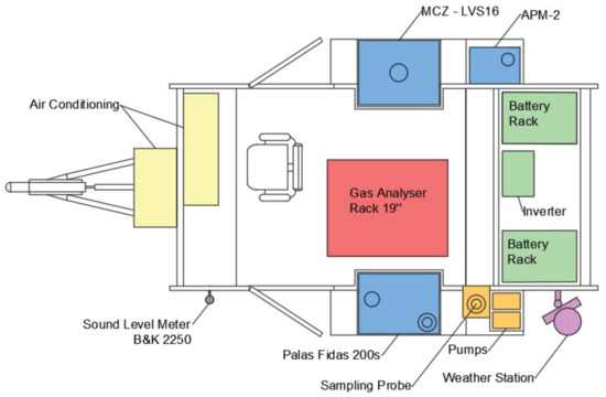
Figure 1.
cc-TrAIRer plan view: locations of instruments and auxiliary systems.
As the Hero Camper is originally intended for travelling, some structural changes were made to adapt it to the instruments’ requirements for research purposes. The roof window was removed to improve the thermal insulation of the vehicle, decreasing the potential heat losses. For the same reason, all the holes that allow the electrical, hydraulic and cable connections through the walls were properly assembled. The kitchen facilities on the back side were taken off to obtain exploitable space where the batteries packs were placed. A support surface was built as a workstation and the personal computer and the datalogger placed there. Additionally, a recess for each side of the trailer was created to externally place different PM analysers. The symmetrical positioning of these two instruments with respect to the trailer’s axis significantly helps to optimize the weight distribution. Indeed, a specific analysis of the load distribution was undertaken to ensure the vehicle stability, paying particular attention to the heaviest elements (such as the rack, the batteries and the air conditioning system). Finally, the majority of the apparatus is located at the centre of the back of the trailer in order to transfer the load to the tires and two rear stabilizers and not exceed the load limit on the hitch.
The baggage rack was used as a support base for the photovoltaic system. The latter was placed horizontally to optimize the electricity generation and to contribute to the aerodynamic shape of the trailer while travelling. However, when solar power is needed to support the functioning of the instrumentation during sampling campaigns, the panels can expand to increase the exposure surface. To stabilize the trailer, they can also be fastened to the soil to avoid the raising of the entire vehicle due to external events.
3.3. Instrumentation
The cc-TrAIRer provides measurements of PM, gases and weather conditions. Table 4 gives an overview of all instruments’ technical specifications. The measurement techniques are described below.
3.3.1. Palas Fidas 200s
The Palas Fidas 200s (Palas GmbH, Karlsruhe, Germany) is an optical analyser with a continuous monitoring system for fine particles in the size range of 180 nm–18 μm. The particle size diameter is computed using Lorenz–Mie scattered light analysis. The instrument provides PM2.5 and PM10 measurements in accordance with the law and others fractions that are useful for research purposes (PM1, PM4, PMtot, particle number concentration Cn and particle size distribution). The instrument has been tested and certified according to the standards VDI 4202-1 (2010), VDI 4203-3 (2010), EN 12341 (1998), EN 14907 (2005), the Guide of Demonstration of Equivalence of Ambient Air Monitoring Methods (2005), EN 15267-1 (2009) and EN 15267-2 (2009). The inlet system is made up of a Sigma-2 sampling head and an Intelligent Aerosol Drying System (IADS). A dried flow is ensured according to the external temperature, humidity and pressure measured by the weather station in order to avoid data acquisition errors due to condensation [95]. The number of monitored parameters and the high temporal resolution of this instrument justify its presence inside the cc-TrAIRer.
3.3.2. APM-2
The Air Pollution Monitor APM-2 (Comde-Derenda GmbH, Stahnsdorf, Germany) is a particle optical analyser for the detection of PM10 and PM2.5 fractions. The instrument has been tested to guarantee its compliance with VDI 4202-1 (2010), VDI 4203-3 (2010), EN 12341 (1998), EN 14907 (2005), the Guide of Demonstration of Equivalence of Ambient Air Monitoring Methods (2010), EN 15267-1 (2009) and EN 15267-2 (2009). The incoming flow is divided into two flows (PM10 and PM2.5) by a virtual impactor with a perpendicular jet. Then, the two flows move alternately through the scattered light photometer unit, where particles are illuminated by a laser diode. The particle size is obtained as a function of the scattered light detected from the photodetector [96].
3.3.3. MicroPNS LVS16
The MicroPNS Type LVS16 (Umwelttechnik MCZ GmbH, Bad Nauheim, Germany) is a PM sequential sampler. All of the instrument specifications are in accordance with EN 12341:2014. The particle collection takes place in an automatic way through 16 filters with diameters of 47 mm. An on-field operation by a qualified staff member is required after 16 days to replace the membranes. The sampler is able to collect just a single fraction (PM10, PM2.5 or TSP) at a time, depending on the inlet head that is assembled [97]. The collected specimens are weighed and examined in order to perform chemical and gravimetric analyses.
3.3.4. Serinus 40 NOx Analyser
The Serinus 40 (Ecotech Pty Ltd., Knoxfield, Australia) is a gas analyser that uses the gas phase chemiluminiscence method to detect nitric oxide (NO), total oxides of nitrogen (NOx) and nitrogen dioxide (NO2) in the range of 0–20 ppm [98]. The instrument has been tested and found to comply with VDI 4202-1 (2010), VDI 4203-3 (2010), EN 14211 (2012), EN 15267-1 (2009) and EN 15267-2 (2009), according to its US EPA approval (RFNA–0809–186) and EN approval (TÜV 936/21221977/A). The ambient air is collected through the sampling probe described below. The auxiliary pump of the analyser is located outside the trailer to reduce the amount of power needed for air conditioning, while the instrument is placed inside the rack to guarantee suitable operation conditions.
3.3.5. Serinus 10 O3 Analyser
The Serinus 10 (Ecotech Pty Ltd., Knoxfield, Australia) is a gas analyser for the detection of Ozone (O3) in the range of 0–20 ppm that uses non-dispersive ultraviolet (UV) absorption technology [99]. The instrument has been tested and found to comply with VDI 4202-1 (2010), EN 14625 (2012), EN 15267-1 (2009) and EN 15267-2 (2009) according to the US EPA approval (EQOA–0809–187) and EN approval (TÜV 936/21221977/C). As for the Serinus 40, the ambient air is collected through the sampling probe described below. Despite the instrument being equipped with an internal pump, the optimization of the trailer temperature required the relocation of the pump in an external arrangement. Due to the potential ozone influence on the other data acquisitions, the instrument was placed above the Serinus 40 in the analyser rack.
3.3.6. Sampling Probe
The gases sampling probe (Sartec—Saras Srl, Milan, Italy) collects the ambient air to send it to the specific pollutant analysers. The air is taken by the sampling head and it moves to the heating probe system, which heats the flux and keeps it over the dew sample point to avoid condensation formation. To prevent the gases’ absorption on the inner wall, the internal channel is insulated and made of PTFE, and a suction fan is installed in the lower part to guarantee the required residence time. The distribution system, consisting of a manifold, allows the connection of up to 12 analysers by Teflon pipes.
3.3.7. Davis Vantage Pro 2 Weather Station
The Davis Vantage Pro 2 (Davis Instruments, Hayward, CA, USA) enables surveying of the main weather conditions. It includes several sensors and devices gathered in a versatile integrated suite. The anemometer is separately installed and it provides both the wind direction and wind speed. The main body of the station consists of a rain collector, temperature and humidity sensors placed inside radiation shields and solar radiation and UV sensors. The weather station also provides other relevant indices, such as the wind chill, heat index, THW index, YHSW index, evapotranspiration and dew point [100].
3.3.8. Sound-Level Meter (Noise)
The sound-level meter used for the acoustic acquisitions is a Bruel Kjaer, Nærum, Denmark, type 2250. The device is class 1 according to international standards. The sound pressure is collected by the microphone, which is screened off by a windscreen, and is sent to the microphone preamplifier. The entire detection structure can be directly linked to the handheld analyser or it can be extended up to 100 m thanks to a small tripod. In this way, the sound-level meter can also be easily managed in the cc-TrAIRer design when a remote location for the microphone is needed. The sound-level meter records the A-weighted sound pressure level to obtain the time history of acquisition campaigns [101].
3.4. Power Supply and Air Conditioning System
The power autonomy of the cc-TrAIRer is ensured by the possibility of its connection to the traditional power network, which should give the needed power consumption of 3 kW. When the electrical grid is not available, the photovoltaic off-grid system is sufficient for all the operational activities from a power point of view. To meet electrical safety standards, the installed contactor is able to immediately cut off the power supply in cases of system or single instrument failures. It can also intervene if the fire protection temperature limit is exceeded.
The photovoltaic system is made up of seven top-efficiency solar panels (Sunpower Maxeon 3400 W) with a parallel connection. They can also be used in a limited configuration, which guarantees the proper functioning of some panels when the others are not expanded. The MPPT solar charge controller (SmartSolar MPPT 150/60-Tr, Victron Energy Almere, The Netherlands) manages the panels’ inverter connections and maintains operation at the maximum power point in order to improve the system efficiency. The multifunctional inverter/charger (Multiplus-II 48/5000/70-50, Victron Energy Almere, The Netherlands) charges the battery pack to 48 V DC and produces 230 V AC to supply the device loads (including instrumentation and air conditioning). The power storage apparatus consists of four 48 V/50 Ah lithium batteries (Pylontech US2000B Plus, Pudong, Shanghai, China).
Particles instruments are designed for external conditions, but gas analysers have an operational temperature range (15–30 °C) that demands an accurate air conditioning design. The cc-TrAIRer was designed to be capable of carrying out sampling campaigns in remote places with critical thermal conditions (such as mountains or particularly dry climate areas).
A preliminary evaluation of the heating load to be removed from the inside of the trailer was undertaken, converting the energy absorbed by the devices into heat. This led to the estimation of a value in BTUs (British thermal units) that would be needed at a minimum. The internal volume of about 6 m3 and the heat produced by the instruments led to the requirement of about 4000–4500 BTU in this study. During the trailer design, some expedient measures were adopted to reduce the device heat stress, which adds a burden to the total amount of needed BTUs. In fact, the analyser pumps were moved outside the trailer to a purpose-built section that protects them from external weather agents.
The selected air conditioner (Fujitsu ASYG07KGTA, nominal power: 400–500 W) is quite small and it was placed in the front side of the trailer in order to provide the flow homogeneously all over the trailer, without directly affecting the analysers. The external unit is located outside, near the internal one.
3.5. Data Management
To optimize the analysis performance and to achieve a suitable parameter overview, a data management system was designed. The cc-TrAIRer is equipped with an operator station where a central data acquisition computer is placed. All the instruments are connected to the computer through a multiport device for serial RS-232 and LAN transmission.
Acquired data are then shared online thanks to a Router RUT240 LTE, Teltonika, Kaunas, Lithuania, which exploits an UMTS system. It provides an internet connection with an external SIM to all the equipment through Ethernet cables or a wireless network. Therefore, the data simultaneously collected by all the instruments are generally sent in real time to a server to allow remote control of the parameter trend. Potential internet signal failure is not a limitation of the mobile laboratory, since all the measurements are always locally stored before being sent online.
Data undergo initial pre-processing before reaching the server. Indeed, their structure is organised to guarantee smart visualisation and data are averaged across a time frame that can be set according to the operator’s choice. A following tool is used to perform the diagnostic phase of the process, highlighting potential errors during the sampling operation. It also allows the insertion of the data in an integrated database and it displays graphical evaluations for the subsequent analysis.
The datalogger also develops reports on potential instrument or system failures. An alert is sent to the operator on different occasions, such as in cases of power breakdown, temperature range errors, exceeding of critical thresholds or other operational condition faults.
The possible implementation of other instruments in the trailer can be easily managed with the central computer of the mobile laboratory, since it can be quickly commanded by the system with the remote connection.
4. Measurement Applications
The cc-TrAIRer has several potential research applications. It can be used to promptly intervene in emergency situations or to identify the impact of local sources on air quality. Moreover, the laboratory can also monitor pollutants’ temporal and spatial distribution in heterogeneous contexts in long term campaigns. These different uses have already been strongly documented by different sampling studies conducted by the research group in the last few years (e.g., [102]). These surveys led to an understanding of the necessity of a complete monitoring laboratory for the integrated study of air pollution. In fact, the conception of the cc-TrAIRer was strongly influenced by the aim of bridging the gaps in previous studies and implementing new investigations, such as the simultaneous detection of meteoclimatic conditions and gas concentration. In this section, the results of some of the most relevant surveys for this purpose are reported. The sampling studies described here analysed PM concentrations using the instruments that were chosen for the moving laboratory.
Immediate-response air quality monitoring was carried out during an emergency situation in which an industrial site caught fire. The intervention was demanded by the local municipality and had to meet their requirements in addition to the conventional sampling points of public agencies. The study (5 April 2019–13 May 2019) was performed in two areas in Piedmont (Italy), at the foot of the Alps, with the aim of studying the phenomena in order to justify the hazes observed by the citizens, although the public institutions reported concentration values lower than limits. In fact, an assessment of the fire development and of the effects of boundary conditions on the daily variability of haze and pollutant concentrations was conducted with high frequency measurements. An APM-2 analyser was used to determine PM2.5 and PM10 trends, initially at a distance of about 3.7 km (days 1–2: Cantalupa) from the burnt site, as shown in Figure 2. Then, the instrument was progressively moved closer to the industrial area (2.2 km, days 3–8: Frossasco 1; 200 m, days 8–40: Frossasco 2).
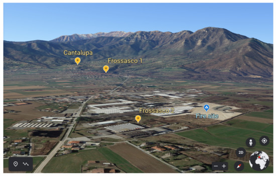
Figure 2.
Location of the fire site and of the Cantalupa, Frossasco 1 and Frossasco 2 sampling points.
A predominant daily trend influenced by the fire event was identified in the initial sampling period. In Figure 3, the most relevant days are shown. The concentration peak detected in the temporal range 10 AM–1 PM was the effect of the mountain and valley breeze, typical of that period of the day due to the local morphology (see Figure 2) [103]. This morning wind contributed to the transportation of the hazes from the burnt site to the sampling stations, which were at higher elevations with respect to the industrial site. This trend faded over the course of the time thanks to the progressive extinction of the fire. As a general remark, although the PM10 daily mean concentration was within the EU air quality standards (2008/50/EC), the identified peaks entailed potential exposure to high values of PM. The analysis was performed in a preliminary way and only obtained the PM distribution, but other implementations for trace gas concentrations in comparable fire situations will be carried out with the future application of the cc-TrAIRer.
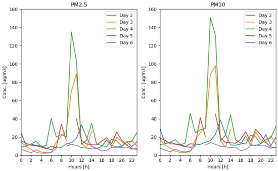
Figure 3.
PM2.5 and PM10 daily trends for the Cantalupa (day 2) and Frossasco (days 3–6) monitoring campaigns. The graphs highlight a predominant peak in the temporal range 10 AM–1 PM.
Another purpose of the APM-2 campaigns was achieved at the mountain site of Salbertrand (Alps, Piedmont, Italy—coordinates: 45.070964, 6.887413). The area was supervised to detect the influence of an anthropic source on the PM local distribution. In fact, a wide area close to the monitoring point was designated for the activities of sand and aggregate industries, with a huge material handling. The instrument was placed at a location about 600 m from this area for 5 weeks (25 September 2020–2 November 2020). The extremely high time resolution of the analyser made it possible to accurately assess the concentration distribution during the day. Figure 4 shows the PM10 trend of the entire period. The working activities had a strong influence on the coarser PM fraction, resulting in a repeated morning peak caused by the particle suspension.
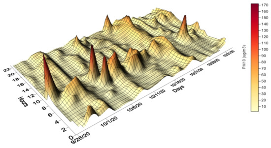
Figure 4.
PM10 hourly trend for the entire period of the Salbertrand monitoring campaign. Frequent peaks can be observed in the morning hours of the day.
To evaluate the PM2.5 and PM10 concentration distribution in different environmental conditions, four monitoring campaigns were performed from June 2019 to March 2020. The sampling points were located in suburban areas at gradually increasing distances from the urban station of Politecnico di Torino, in the direction of the city of Milan (northeast). The array runs along the A4 highway in a flat area of the Po Valley megacity, far from mountains or other high ground. APM-2 analysers were located in the cities of Volpiano, Mazzè and Montanaro, as places identified to have comparable boundary conditions. The details of the single sampling points, concerning the time period and concentration values, are listed in Table 5.
Table 5.
Details of the array monitoring campaign: coordinates, sampling period, means and maximum and minimum values of PM2.5 and PM10.
The results were also compared with the PM trends from the fixed station of Politecnico di Torino in order to observe the difference between urban and suburban areas. Without considering the absolute values, the overall distribution of PM concentrations shows similar trends in urban and suburban sites, suggesting a comparable response to the weather conditions also. Figure 5 shows the difference between the data acquired by the two APM-2s in the external sites and the fixed station. The almost null trend of PM2.5 delta (Figure 5) confirms the results of previous studies [104] regarding the homogeneous spatial distribution of the fine fraction in comparison with the coarse one. PM2.5 values were, in fact, similar in both environmental contexts and in different seasonal conditions. On the contrary, the PM10 trend was affected more by the local situation. As expected, the fixed station values were generally higher than the others, but the Volpiano campaign presented an opposite trend. In this case, the sampled data could not properly be considered as background conditions because of some nearby anthropic activities that had not been considered in the instrument positioning. The material handlings of aggregate industrial work about 400 m away and the people frequently in attendance at the site could have contributed to the high mean value of PM10. Finally, the results of this spatial assessment of the concentration distribution suggest a stronger dependence of the coarser PM fraction on the local sources. For this reason, a suitable preliminary study of sites should be performed to avoid issues in the identification of background trends.
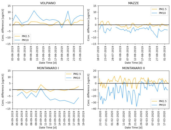
Figure 5.
Differences between the data acquired by the two APM-2s in the external sites and the fixed urban station located in Politecnico di Torino (Turin, Italy). An almost null trend for PM2.5 delta was obtained. The PM10 trend was affected more by the local situation. PM10 suburban station values were generally lower than the fixed one, but the Volpiano campaign presented an opposite trend because of boundary conditions.
The PM assessments were carried out thanks to the great versatility, in terms of repositioning and independence from auxiliary elements, of the APM-2 analyser. The specific thermohygrometric operative conditions of gas analysers and the requirements for sampling accuracy have made gas measurement campaigns with easily movable instruments difficult, up to now, in remote areas. The cc-TrAIRer can guarantee the sampling characteristics needed for all instruments to perform combined gas and particle collections, even those concerning precursor pollutants.
5. Conclusions
We designed and developed a non-motorised, instrumented trailer, the cc-TrAIRer, for high-quality research on air quality and climate changes. The results shown in Section 4 proved the usefulness of this mobile laboratory for simultaneous assessment of several air pollutants along with a mutual correlation of meteoclimatic and environmental conditions.
Thanks to its relatively small dimensions, the trailer is easily transportable to narrow areas, which are of scientific interest but generally not assessed since they are beyond the measurements needs of public agencies. The photovoltaic system encourages its versatility in terms of power supply, allowing sampling campaigns where a relevant infrastructure does not exist. The Alps are a clear example of an area where applications are laborious but, at the same time, key points of research, since they are more strongly exposed than other parts of the Earth to the effects of climate change. Due to the data and system remote management, the technical field interventions can be minimised. The instruments were selected by evaluating their adaptability to the trailer purpose, considering the measured parameters, dimensions, operational conditions, ordinary maintenance and the temporal resolution.
Given the listed advantages, the cc-TrAIRer has potential uses for different research studies, such as those on air compounds’ temporal and spatial distribution or source impacts or emergency situations with short- or long-term campaigns. After a preliminary design plan of the sampling points, an examination of the investigated area should be done to confirm the proper trailer location, taking into account the surrounding environmental dynamics and, at the same time, the accessibility and the safety requirements of the trailer.
Further sampling surveys of the cc-TrAIRer will analyse the reciprocal influences of air compound concentrations, weather and atmospheric and environmental conditions in different land-use contexts, providing considerable support to the investigation of global aspects of climate change.
Author Contributions
Conceptualization, C.B., D.M., F.P. and M.C.; Methodology, C.B., D.M., F.P. and M.C.; Resources, M.B.; Supervision, M.C.; Validation, C.B., D.M., F.P. and M.C.; Visualization, C.B. and D.M.; Writing—original draft, C.B. and D.M.; Writing—review & editing, F.P. and M.C. All authors have read and agreed to the published version of the manuscript.
Funding
Funding of the cc-TrAIRer project was provided by the program “Dipartimenti di Eccellenza 2018–2022” under the climate_change@polito project of the Department of Environmental, Land and Infrastructure Engineering (DIATI) of the Politecnico di Torino.
Institutional Review Board Statement
Not applicable.
Informed Consent Statement
Not applicable.
Data Availability Statement
Not applicable.
Acknowledgments
We would like to thank the municipalities of Cantalupa, Frossasco and Salbertrand for their cooperation. We are also very grateful to Nuova Allcar for the supply in the execution of the trailer.
Conflicts of Interest
The authors declare no conflict of interest.
References
- ONU. Transforming Our World: The 2030 Agenda for Sustainable Development. 2015, pp. 12–14. Available online: https://www.un.org/ga/search/view_doc.asp?symbol=A/RES/70/1&Lang=E (accessed on 3 August 2021). [CrossRef]
- EEA. Climate Change and Air. 2013, pp. 1–8. Available online: https://www.eea.europa.eu/signals/signals-2013/articles/climate-change-and-air (accessed on 3 August 2021).
- IPCC. Chapter 11. Fifth Assessment Report of IPCC. In Climate Change 2014 Impacts, Adaptation, and Vulnerability; 2015; pp. 709–754. Available online: https://archive.ipcc.ch/publications_and_data/ar4/wg1/en/ch11.html (accessed on 3 August 2021). [CrossRef]
- WHO. Ambient Air Pollution: A Global Assesment of Exposure and Burden of Disease; WHO: Geneva, Switzerland, 2016; pp. 68–70. Available online: https://apps.who.int/iris/handle/10665/250141 (accessed on 3 August 2021).
- Landrigan, P.J. Air pollution and health. Lancet Public Health 2017, 2, e4–e5. [Google Scholar] [CrossRef]
- Burnett, R.; Chen, H.; Szyszkowicz, M.; Fann, N.; Hubbell, B.; Pope, C.A.; Apte, J.S.; Brauer, M.; Cohen, A.; Weichenthal, S.; et al. Global estimates of mortality associated with long-term exposure to outdoor fine particulate matter. Proc. Natl. Acad. Sci. USA 2018, 115, 9592–9597. [Google Scholar] [CrossRef]
- Amato, F.; Alastuey, A.; Karanasiou, A.; Lucarelli, F.; Nava, S.; Calzolai, G.; Severi, M.; Becagli, S.; Gianelle, V.L.; Colombi, C.; et al. AIRUSE-LIFE+: A harmonized PM speciation and source apportionment in five southern European cities. Atmos. Chem. Phys. Discuss. 2016, 16, 3289–3309. [Google Scholar] [CrossRef]
- Hu, J.; Wang, H.; Zhang, J.; Zhang, M.; Zhang, H.; Wang, S.; Chai, F. PM2.5 Pollution in Xingtai, China: Chemical Characteristics, Source Apportionment, and Emission Control Measures. Atmosphere 2019, 10, 121. [Google Scholar] [CrossRef]
- Huang, R.-J.; Wang, Y.; Cao, J.; Lin, C.; Duan, J.; Chen, Q.; Li, Y.; Gu, Y.; Yan, J.; Xu, W.; et al. Primary emissions versus secondary formation of fine particulate matter in the most polluted city (Shijiazhuang) in North China. Atmos. Chem. Phys. Discuss. 2019, 19, 2283–2298. [Google Scholar] [CrossRef]
- Mukherjee, A.; Agrawal, M. World air particulate matter: Sources, distribution and health effects. Environ. Chem. Lett. 2017, 15, 283–309. [Google Scholar] [CrossRef]
- Daellenbach, K.R.; Uzu, G.; Jiang, J.; Cassagnes, L.-E.; Leni, Z.; Vlachou, A.; Stefenelli, G.; Canonaco, F.; Weber, S.; Segers, A.; et al. Sources of particulate-matter air pollution and its oxidative potential in Europe. Nature 2020, 587, 414–419. [Google Scholar] [CrossRef]
- Perrino, C.; Canepari, S.; Catrambone, M.; Torre, S.D.; Rantica, E.; Sargolini, T. Influence of natural events on the concentration and composition of atmospheric particulate matter. Atmos. Environ. 2009, 43, 4766–4779. [Google Scholar] [CrossRef]
- Azimi, M.; Feng, F.; Yang, Y. Air Pollution Inequality and Its Sources in SO2 and NOX Emissions among Chinese Provinces from 2006 to 2015. Sustainability 2018, 10, 367. [Google Scholar] [CrossRef]
- Badr, O.; Probert, S. Sources of atmospheric carbon monoxide. Appl. Energy 1994, 49, 145–195. [Google Scholar] [CrossRef]
- Yarragunta, Y.; Srivastava, S.; Mitra, D.; Chandola, H.C. Source apportionment of carbon monoxide over India: A quantitative analysis using MOZART-4. Environ. Sci. Pollut. Res. 2021, 28, 8722–8742. [Google Scholar] [CrossRef]
- Sillman, S. Tropospheric Ozone and Photochemical Smog. In Treatise on Geochemistry; University of Michigan: Ann Arbor, MI, USA; Elsevier Inc.: Amsterdam, The Netherlands, 2003; Volume 9–9, pp. 407–431. [Google Scholar]
- Berezina, E.; Moiseenko, K.; Skorokhod, A.; Pankratova, N.; Belikov, I.; Belousov, V.; Elansky, N. Impact of VOCs and NOx on Ozone Formation in Moscow. Atmosphere 2020, 11, 1262. [Google Scholar] [CrossRef]
- Wang, S.; Kaur, M.; Li, T.; Pan, F. Effect of Different Pollution Parameters and Chemical Components of PM2.5 on Health of Residents of Xinxiang City, China. Int. J. Environ. Res. Public Health 2021, 18, 6821. [Google Scholar] [CrossRef] [PubMed]
- Rückerl, R.; Schneider, A.; Breitner, S.; Cyrys, J.; Peters, A. Health effects of particulate air pollution: A review of epidemiological evidence. Inhal. Toxicol. 2011, 23, 555–592. [Google Scholar] [CrossRef]
- Lipfert, F.W. Long-term associations of morbidity with air pollution: A catalog and synthesis. J. Air Waste Manag. Assoc. 2017, 68, 12–28. [Google Scholar] [CrossRef]
- Sivarethinamohan, R.; Sujatha, S.; Priya, S.; Sankaran; Gafoor, A.; Rahman, Z. Impact of air pollution in health and socio-economic aspects: Review on future approach. Mater. Today Proc. 2021, 37, 2725–2729. [Google Scholar] [CrossRef]
- Robichaud, A.; Comtois, P. Environmental factors and asthma hospitalization in Montreal, Canada, during spring 2006–2008: A synergy perspective. Air Qual. Atmos. Health 2019, 12, 1495–1509. [Google Scholar] [CrossRef]
- Zhang, X.; Chen, X.; Zhang, X. The impact of exposure to air pollution on cognitive performance. Proc. Natl. Acad. Sci. USA 2018, 115, 9193–9197. [Google Scholar] [CrossRef] [PubMed]
- Chua, S.Y.L.; Khawaja, A.P.; Morgan, J.; Strouthidis, N.; Reisman, C.; Dick, A.D.; Khaw, P.T.; Patel, P.J.; Foster, P.J. For the UK Biobank Eye and Vision Consortium The Relationship Between Ambient Atmospheric Fine Particulate Matter (PM2.5) and Glaucoma in a Large Community Cohort. Investig. Opthalmol. Vis. Sci. 2019, 60, 4915–4923. [Google Scholar] [CrossRef] [PubMed]
- Wong, I.C.K.; Ng, Y.-K.; Lui, V.W.Y. Cancers of the lung, head and neck on the rise: Perspectives on the genotoxicity of air Pollution. Chin. J. Cancer 2014, 33, 476–480. [Google Scholar] [CrossRef]
- Brook, R.D.; Rajagopalan, S.; Pope, C.A.; Brook, J.R.; Bhatnagar, A.; Diez-Roux, A.V.; Holguin, F.; Hong, Y.; Luepker, R.V.; Mittleman, M.A.; et al. Particulate Matter Air Pollution and Cardiovascular Disease: An update to the scientific statement from the american heart association. Circulation 2010, 121, 2331–2378. [Google Scholar] [CrossRef] [PubMed]
- Baja, E.S.; Schwartz, J.D.; Wellenius, G.; Coull, B.A.; Zanobetti, A.; Vokonas, P.S.; Suh, H. Traffic-Related Air Pollution and QT Interval: Modification by Diabetes, Obesity, and Oxidative Stress Gene Polymorphisms in the Normative Aging Study. Environ. Health Perspect. 2010, 118, 840–846. [Google Scholar] [CrossRef] [PubMed]
- Zhang, X.; Battiston, K.G.; Labow, R.S.; Simmons, C.A.; Santerre, J.P. Generating favorable growth factor and protease release profiles to enable extracellular matrix accumulation within an in vitro tissue engineering environment. Acta Biomater. 2017, 54, 81–94. [Google Scholar] [CrossRef] [PubMed]
- Burns, D.A.; Aherne, J.; Gay, D.A.; Lehmann, C.M. Acid rain and its environmental effects: Recent scientific advances. Atmos. Environ. 2016, 146, 1–4. [Google Scholar] [CrossRef]
- Sun, X.; Zhao, T.; Liu, D.; Gong, S.; Xu, J.; Ma, X. Quantifying the Influences of PM2.5 and Relative Humidity on Change of Atmospheric Visibility over Recent Winters in an Urban Area of East China. Atmosphere 2020, 11, 461. [Google Scholar] [CrossRef]
- Wu, Y.; Zhang, J.; Liu, S.; Jiang, Z.; Arbi, I.; Huang, X.; Macreadie, P.I. Nitrogen deposition in precipitation to a monsoon-affected eutrophic embayment: Fluxes, sources, and processes. Atmos. Environ. 2018, 182, 75–86. [Google Scholar] [CrossRef]
- Manisalidis, I.; Stavropoulou, E.; Stavropoulos, A.; Bezirtzoglou, E. Environmental and Health Impacts of Air Pollution: A Review. Front. Public Health 2020, 8, 14. [Google Scholar] [CrossRef] [PubMed]
- Ramanathan, V.; Carmichael, G. Global and regional climate changes due to black carbon. Nat. Geosci. 2008, 1, 221–227. [Google Scholar] [CrossRef]
- Shrestha, G.; Traina, S.J.; Swanston, C.W. Black Carbon’s Properties and Role in the Environment: A Comprehensive Review. Sustainability 2010, 2, 294–320. [Google Scholar] [CrossRef]
- Jacob, D.J.; Winner, D.A. Effect of climate change on air quality. Atmos. Environ. 2009, 43, 51–63. [Google Scholar] [CrossRef]
- Christensen, J.H.; Hewitson, B.; Busuioc, A.; Chen, A.; Gao, X.; Held, I.; Jones, R.; Kolli, R.K.; Kwon, W.T.; Laprise, R.; et al. Regional Climate Projections; Climate Change 2007: The Physical Science Basis. Contribution of Working Group I to the Fourth Assessment Report of the Intergovernmental Panel on ClimateChange; Chapter 11; Cambridge University Press: Cambridge, UK; New York, NY, USA, 2007. [Google Scholar]
- Horton, D.; Skinner, C.; Singh, D.; Diffenbaugh, N. Occurrence and persistence of future atmospheric stagnation events. Nat. Clim. Chang. 2014, 4, 698–703. [Google Scholar] [CrossRef] [PubMed]
- Chang, H.H.; Zhou, J.; Fuentes, M. Impact of Climate Change on Ambient Ozone Level and Mortality in Southeastern United States. Int. J. Environ. Res. Public Health 2010, 7, 2866–2880. [Google Scholar] [CrossRef] [PubMed]
- Orru, H.; Andersson, C.; Ebi, K.L.; Langner, J.; Åström, C.; Forsberg, B. Impact of climate change on ozone-related mortality and morbidity in Europe. Eur. Respir. J. 2012, 41, 285–294. [Google Scholar] [CrossRef] [PubMed]
- Karlsson, P.E.; Klingberg, J.; Engardt, M.; Andersson, C.; Langner, J.; Karlsson, G.P.; Pleijel, H. Past, present and future concentrations of ground-level ozone and potential impacts on ecosystems and human health in northern Europe. Sci. Total. Environ. 2017, 576, 22–35. [Google Scholar] [CrossRef] [PubMed]
- Cooper, R.N.; Houghton, J.T.; McCarthy, J.J.; Metz, B. Climate Change 2001: The Scientific Basis. Foreign Aff. 2002, 81, 208. [Google Scholar] [CrossRef]
- Beniston, M. Mountain Weather and Climate: A General Overview and a Focus on Climatic Change in the Alps. Hydrobiologia 2006, 562, 3–16. [Google Scholar] [CrossRef]
- Bo, M.; Salizzoni, P.; Pognant, F.; Mezzalama, R.; Clerico, M. A Combined Citizen Science—Modelling Approach for NO2 Assessment in Torino Urban Agglomeration. Atmosphere 2020, 11, 721. [Google Scholar] [CrossRef]
- Bada, J.L.; Zent, A.P.; Grunthaner, F.J.; Quinn, R.C.; Navarro-Gonzalez, R.; Gomez-Silva, B.; McKay, C.P.; Baker, V.R.; Bandfield, J.L.; Banerdt, W.B.; et al. Astrobiolab: A mobile biotic and soil analysis laboratory. In Proceedings of the Sixth International Conference on Mars, Pasadena, CA, USA, 1 January 2003. [Google Scholar]
- Brantley, H.L.; Hagler, G.; Kimbrough, E.S.; Williams, R.W.; Mukerjee, S.; Neas, L.M. Mobile air monitoring data-processing strategies and effects on spatial air pollution trends. Atmos. Meas. Tech. 2014, 7, 2169–2183. [Google Scholar] [CrossRef]
- Berk, J.; Hollowell, C.; Lin, C.; Pepper, J. Design of A Mobile Laboratory for Ventilation Studies and Indoor Air Pollution Monitoring; Energy and Environment Division; Lawrence Berkeley Lab.: Berkeley, CA, USA, 1978. [Google Scholar] [CrossRef][Green Version]
- Bukowiecki, N.; Dommen, J.; Prévôt, A.; Richter, R.; Weingartner, E.; Baltensperger, U. A mobile pollutant measurement laboratory—measuring gas phase and aerosol ambient concentrations with high spatial and temporal resolution. Atmos. Environ. 2002, 36, 5569–5579. [Google Scholar] [CrossRef]
- Pirjola, L.; Lähde, T.; Niemi, J.; Kousa, A.; Rönkkö, T.; Karjalainen, P.; Keskinen, J.; Frey, A.; Hillamo, R. Spatial and temporal characterization of traffic emissions in urban microenvironments with a mobile laboratory. Atmos. Environ. 2012, 63, 156–167. [Google Scholar] [CrossRef]
- Zhu, Y.; Zhang, J.; Wang, J.; Chen, W.; Han, Y.; Ye, C.; Li, Y.; Liu, J.; Zeng, L.; Wu, Y.; et al. Distribution and sources of air pollutants in the North China Plain based on on-road mobile measurements. Atmos. Chem. Phys. Discuss. 2016, 16, 12551–12565. [Google Scholar] [CrossRef]
- Kittelson, D.; Johnson, J.; Watts, W.; Wei, Q.; Drayton, M.; Paulsen, D.; Bukowiecki, N. Diesel Aerosol Sampling in the Atmosphere. SAE Tech. Paper Series 2000. [Google Scholar] [CrossRef]
- Elanskii, N.F.; Belikov, I.B.; Golitsyn, G.S.; Grisenko, A.M.; Lavrova, O.V.; Pankratova, N.V.; Safronov, A.N.; Skorokhod, A.I.; Shumskii, R.A. Observations of the atmosphere composition in the Moscow megapolis from a mobile laboratory. Dokl. Earth Sci. 2010, 432, 649–655. [Google Scholar] [CrossRef]
- Hagemann, R.; Corsmeier, U.; Kottmeier, C.; Rinke, R.; Wieser, A.; Vogel, B. Spatial variability of particle number concentrations and NOx in the Karlsruhe (Germany) area obtained with the mobile laboratory ‘AERO-TRAM’. Atmos. Environ. 2014, 94, 341–352. [Google Scholar] [CrossRef]
- Petäjä, T.; Vakkari, V.; Pohja, T.; Nieminen, T.; Laakso, H.; Aalto, P.; Keronen, P.; Siivola, E.; Kerminen, V.-M.; Kulmala, M.; et al. Transportable Aerosol Characterization Trailer with Trace Gas Chemistry: Design, Instruments and Verification. Aerosol Air Qual. Res. 2013, 13, 421–435. [Google Scholar] [CrossRef]
- Westerdahl, D.; Fruin, S.; Sax, T.; Fine, P.M.; Sioutas, C. Mobile platform measurements of ultrafine particles and associated pollutant concentrations on freeways and residential streets in Los Angeles. Atmos. Environ. 2005, 39, 3597–3610. [Google Scholar] [CrossRef]
- Tang, U.W.; Wang, Z. Determining gaseous emission factors and driver’s particle exposures during traffic congestion by vehicle-following measurement techniques. J. Air Waste Manag. Assoc. 2006, 56, 1532–1539. [Google Scholar] [CrossRef]
- Kuhns, H.; Etyemezian, V.; Landwehr, D.; MacDougall, C.; Pitchford, M.; Green, M. Testing Re-entrained Aerosol Kinetic Emissions from Roads: A new approach to infer silt loading on roadways. Atmos. Environ. 2001, 35, 2815–2825. [Google Scholar] [CrossRef]
- Elen, B.; Peters, J.; Van Poppel, M.; Bleux, N.; Theunis, J.; Reggente, M.; Standaert, A. The Aeroflex: A Bicycle for Mobile Air Quality Measurements. Sensors 2012, 13, 221–240. [Google Scholar] [CrossRef]
- Farrell, P.; Culling, D.; Leifer, I. Transcontinental methane measurements: Part 1. A mobile surface platform for source investigations. Atmos. Environ. 2013, 74, 422–431. [Google Scholar] [CrossRef]
- Leifer, I.; Culling, D.; Schneising, O.; Farrell, P.; Buchwitz, M.; Burrows, J.P. Transcontinental methane measurements: Part 2. Mobile surface investigation of fossil fuel industrial fugitive emissions. Atmos. Environ. 2013, 74, 432–441. [Google Scholar] [CrossRef]
- Padró-Martínez, L.T.; Patton, A.; Trull, J.B.; Zamore, W.; Brugge, D.; Durant, J.L. Mobile monitoring of particle number concentration and other traffic-related air pollutants in a near-highway neighborhood over the course of a year. Atmos. Environ. 2012, 61, 253–264. [Google Scholar] [CrossRef]
- Dominici, F.; Peng, R.D.; Bell, M.; Pham, L.; McDermott, A.; Zeger, S.L.; Samet, J.M. Fine Particulate Air Pollution and Hospital Admission for Cardiovascular and Respiratory Diseases. JAMA 2006, 295, 1127–1134. [Google Scholar] [CrossRef]
- Yang, H.-J.; Liu, X.; Qu, C.; Shi, S.-B.; Liang, J.-J.; Yang, B. Main air pollutants and ventricular arrhythmias in patients with implantable cardioverter-defibrillators: A systematic review and meta-analysis. Chronic Dis. Transl. Med. 2017, 3, 242–251. [Google Scholar] [CrossRef]
- Enyoh, C.E.; Verla, A.W.; Qingyue, W.; Ohiagu, F.O.; Chowdhury, A.H.; Enyoh, E.C.; Chowdhury, T.; Verla, E.N.; Chinwendu, U.P. An overview of emerging pollutants in air: Method of analysis and potential public health concern from human environmental exposure. Trends Environ. Anal. Chem. 2020, 28, e00107. [Google Scholar] [CrossRef]
- Bush, S.E.; Hopkins, F.M.; Randerson, J.T.; Lai, C.-T.; Ehleringer, J.R. Design and application of a mobile ground-based observatory for continuous measurements of atmospheric trace gas and criteria pollutant species. Atmos. Meas. Tech. 2015, 8, 3481–3492. [Google Scholar] [CrossRef]
- Phillips, N.G.; Ackley, R.; Crosson, E.R.; Down, A.; Hutyra, L.R.; Brondfield, M.; Karr, J.D.; Zhao, K.; Jackson, R.B. Mapping urban pipeline leaks: Methane leaks across Boston. Environ. Pollut. 2013, 173, 1–4. [Google Scholar] [CrossRef] [PubMed]
- Jackson, R.B.; Down, A.; Phillips, N.G.; Ackley, R.C.; Cook, C.W.; Plata, D.L.; Zhao, K. Natural Gas Pipeline Leaks Across Washington, DC. Environ. Sci. Technol. 2014, 48, 2051–2058. [Google Scholar] [CrossRef]
- Tao, L.; Sun, K.; Miller, D.J.; Pan, D.; Golston, L.M.; Zondlo, M.A. Low-power, open-path mobile sensing platform for high-resolution measurements of greenhouse gases and air pollutants. Appl. Phys. A 2015, 119, 153–164. [Google Scholar] [CrossRef]
- Isakov, V.; Touma, J.S.; Khlystov, A. A method of assessing air toxics concentrations in urban areas using mobile platform measurements. J. Air Waste Manag. Assoc. 2007, 57, 1286–1295. [Google Scholar] [CrossRef]
- Shorter, J.H.; McManus, J.B.; Kolb, C.E.; Allwine, E.J.; Lamb, B.K.; Mosher, B.W.; Harriss, R.C.; Partchatka, U.; Fischer, H.; Harris, G.W.; et al. Methane emission measurements in urban areas in Eastern Germany. J. Atmos. Chem. 1996, 24, 121–140. [Google Scholar] [CrossRef]
- Weimer, S.; Mohr, C.; Richter, R.; Keller, J.; Mohr, M.; Prévôt, A.; Baltensperger, U. Mobile measurements of aerosol number and volume size distributions in an Alpine valley: Influence of traffic versus wood burning. Atmos. Environ. 2009, 43, 624–630. [Google Scholar] [CrossRef]
- Wang, M.; Zhu, T.; Zhang, J.P.; Zhang, Q.H.; Lin, W.W.; Li, Y.; Wang, Z.F. Using a mobile laboratory to characterize the distribution and transport of sulfur dioxide in and around Beijing. Atmos. Chem. Phys. Discuss. 2011, 11, 11631–11645. [Google Scholar] [CrossRef]
- Czarnecka, M.; Nidzgorska-Lencewicz, J. Impact of weather conditions on winter and summer air quality. Int. Agrophysics 2011, 25, 7–12. [Google Scholar]
- Ning, G.; Yim, S.H.L.; Wang, S.; Duan, B.; Nie, C.; Yang, X.; Wang, J.; Shang, K. Synergistic effects of synoptic weather patterns and topography on air quality: A case of the Sichuan Basin of China. Clim. Dyn. 2019, 53, 6729–6744. [Google Scholar] [CrossRef]
- Schneider, J.; Kirchner, U.; Borrmann, S.; Vogt, R.; Scheer, V. In situ measurements of particle number concentration, chemically resolved size distributions and black carbon content of traffic-related emissions on German motorways, rural roads and in city traffic. Atmos. Environ. 2008, 42, 4257–4268. [Google Scholar] [CrossRef]
- Maciejczyk, P.B.; Offenberg, J.H.; Clemente, J.; Blaustein, M.; Thurston, G.D.; Chen, L.C. Ambient pollutant concentrations measured by a mobile laboratory in South Bronx, NY. Atmos. Environ. 2004, 38, 5283–5294. [Google Scholar] [CrossRef]
- Wang, M.; Zhu, T.; Zheng, J.; Zhang, R.; Zhang, S.Q.; Xie, X.X.; Han, Y.Q.; Li, Y. Use of a mobile laboratory to evaluate changes in on-road air pollutants during the Beijing 2008 Summer Olympics. Atmos. Chem. Phys. Discuss. 2009, 9, 8247–8263. [Google Scholar] [CrossRef]
- Zhang, J.; Ninneman, M.; Joseph, E.; Schwab, M.J.; Shrestha, B.; Schwab, J.J. Mobile Laboratory Measurements of High Surface Ozone Levels and Spatial Heterogeneity During LISTOS 2018: Evidence for Sea Breeze Influence. J. Geophys. Res. Atmos. 2020, 125. [Google Scholar] [CrossRef]
- Gröbner, J.; Blumthaler, M.; Kazadzis, S.; Bais, A.; Webb, A.; Schreder, J.; Seckmeyer, G.; Rembges, D. Quality assurance of spectral solar UV measurements: Results from 25 UV monitoring sites in Europe, 2002 to 2004. Metrologia 2006, 43, S66–S71. [Google Scholar] [CrossRef]
- Ionel, I.; Popescu, F. Data acquisition system in a mobile air quality monitoring station. In Proceedings of the 2009 5th International Symposium on Applied Computational Intelligence and Informatics, Timisoara, Romania, 28–29 May 2009; pp. 557–562. [Google Scholar] [CrossRef]
- Pirjola, L.; Parviainen, H.; Hussein, T.; Valli, A.; Hämeri, K.; Aaalto, P.; Virtanen, A.; Keskinen, J.; Pakkanen, T.; Mäkelä, T.; et al. “Sniffer”—A novel tool for chasing vehicles and measuring traffic pollutants. Atmos. Environ. 2004, 38, 3625–3635. [Google Scholar] [CrossRef]
- Canagaratna, M.R.; Jayne, J.T.; Ghertner, D.A.; Herndon, S.; Shi, Q.; Jimenez, J.L.; Silva, P.; Williams, P.; Lanni, T.; Drewnick, F.; et al. Chase Studies of Particulate Emissions from in-use New York City Vehicles. Aerosol Sci. Technol. 2004, 38, 555–573. [Google Scholar] [CrossRef]
- Von Der Weiden-Reinmüller, S.-L.; Drewnick, F.; Crippa, M.; Prevot, A.; Meleux, F.; Baltensperger, U.; Beekmann, M.; Borrmann, S. Application of mobile aerosol and trace gas measurements for the investigation of megacity air pollution emissions: The Paris metropolitan area. Atmos. Meas. Tech. 2014, 7, 279–299. [Google Scholar] [CrossRef]
- Wallace, J.; Corr, D.; DeLuca, P.; Kanaroglou, P.; McCarry, B. Mobile monitoring of air pollution in cities: The case of Hamilton, Ontario, Canada. J. Environ. Monit. 2009, 11, 998–1003. [Google Scholar] [CrossRef]
- Levy, I.; Mihele, C.; Lu, G.; Narayan, J.; Hilker, N.; Brook, J.R. Elucidating multipollutant exposure across a complex metropolitan area by systematic deployment of a mobile laboratory. Atmos. Chem. Phys. Discuss. 2014, 14, 7173–7193. [Google Scholar] [CrossRef]
- Hussein, T.; Johansson, C.; Karlsson, H.; Hansson, H.-C. Factors affecting non-tailpipe aerosol particle emissions from paved roads: On-road measurements in Stockholm, Sweden. Atmos. Environ. 2008, 42, 688–702. [Google Scholar] [CrossRef]
- Cocker, D.R.; Shah, S.D.; Johnson, K.; Miller, J.W.; Norbeck, J.M. Development and Application of a Mobile Laboratory for Measuring Emissions from Diesel Engines. 1. Regulated Gaseous Emissions. Environ. Sci. Technol. 2004, 38, 2182–2189. [Google Scholar] [CrossRef]
- Borrego, C.; Costa, A.m.; Ginja, J.; Amorim, M.; Coutinho, M.; Karatzas, K.; Sioumis, T.; Katsifarakis, N.; Konstantinidis, K.; De Vito, S.; et al. Assessment of air quality microsensors versus reference methods: The EuNetAir joint exercise. Atmos. Environ. 2016, 147, 246–263. [Google Scholar] [CrossRef]
- Mohr, C.; Richter, R.; DeCarlo, P.; Prevot, A.; Baltensperger, U. Spatial variation of chemical composition and sources of submicron aerosol in Zurich during wintertime using mobile aerosol mass spectrometer data. Atmos. Chem. Phys. Discuss. 2011, 11, 7465–7482. [Google Scholar] [CrossRef]
- Drewnick, F.; Böttger, T.; Von Der Weiden-Reinmüller, S.-L.; Zorn, S.R.; Klimach, T.; Schneider, J.; Borrmann, S. Design of a mobile aerosol research laboratory and data processing tools for effective stationary and mobile field measurements. Atmos. Meas. Tech. 2012, 5, 1443–1457. [Google Scholar] [CrossRef]
- Kolb, C.E.; Herndon, S.C.; McManus, J.B.; Shorter, J.H.; Zahniser, M.S.; Nelson, D.D.; Jayne, J.T.; Canagaratna, M.R.; Worsnop, D.R. Mobile Laboratory with Rapid Response Instruments for Real-Time Measurements of Urban and Regional Trace Gas and Particulate Distributions and Emission Source Characteristics. Environ. Sci. Technol. 2004, 38, 5694–5703. [Google Scholar] [CrossRef]
- Zavala, M.; Herndon, S.C.; Slott, R.S.; Dunlea, E.J.; Marr, L.C.; Shorter, J.H.; Zahniser, M.; Knighton, W.B.; Rogers, T.M.; Kolb, C.E.; et al. Characterization of on-road vehicle emissions in the Mexico City Metropolitan Area using a mobile laboratory in chase and fleet average measurement modes during the MCMA-2003 field campaign. Atmos. Chem. Phys. Discuss. 2006, 6, 5129–5142. [Google Scholar] [CrossRef]
- Etyemezian, V.; Kuhns, H.; Gillies, J.; Green, M.; Pitchford, M.; Watson, J. Vehicle-based road dust emission measurement: I—Methods and calibration. Atmos. Environ. 2003, 37, 4559–4571. [Google Scholar] [CrossRef]
- Fecht, D.; Hansell, A.; Morley, D.; Dajnak, D.; Vienneau, D.; Beevers, S.; Toledano, M.B.; Kelly, F.J.; Anderson, H.R.; Gulliver, J. Spatial and temporal associations of road traffic noise and air pollution in London: Implications for epidemiological studies. Environ. Int. 2016, 88, 235–242. [Google Scholar] [CrossRef]
- Sun, H.; Gui, D.; Yan, B.; Liu, Y.; Liao, W.; Zhu, Y.; Lu, C.; Zhao, N. Assessing the potential of random forest method for estimating solar radiation using air pollution index. Energy Convers. Manag. 2016, 119, 121–129. [Google Scholar] [CrossRef]
- Palas Operating Manual, “Fidas 200s—System”, 2016. Available online: https://www.palas.de/file/3N6047/application/pdf/5200-en_V2.1_0421_Fidas+200_Operating+Manual.pdf (accessed on 3 August 2021).
- Comde Derenda Manual, Air Pollution Monitor APM-2. 2019. Available online: https://www.comde-derenda.com/wp-content/uploads/2016/09/Colombia_db-230-en-APM-2_2021-1.pdf (accessed on 3 August 2021).
- Umwelttechnik MCZ Manual, Sequential Particulate Sampler MicroPNS Type LVS16-Split. Available online: https://www.mcz.de/datenblaetter/LVS16_Split_type_MCZ_leaflet.pdf (accessed on 3 August 2021).
- Ecotech User Manual, Serinus 40 Oxides of Nitrogen Analyser. 2015. Available online: https://www.ecotech.com/wp-content/uploads/2015/01/M010028-Serinus-40-NOx-User-Manual-2.2.pdf (accessed on 3 August 2021).
- Ecotech User Manual, Serinus 10 Ozone Analyser. 2015. Available online: https://www.ecotech.com/wp-content/uploads/2015/01/Serinus-10-Manual-Ver-3.pdf (accessed on 3 August 2021).
- Davis Instruments Manual, Vantage Pro 2. 2020. Available online: https://cdn.shopify.com/s/files/1/0515/5992/3873/files/07395-289_UM_6820.pdf (accessed on 3 August 2021).
- Brüel & Kjær Manual, “Hand-Held Analyser Types 2250 and 2270”, 2016. Available online: https://www.bksv.com/-/media/literature/Various/be1713.ashx (accessed on 3 August 2021).
- Bo, M.; Mercalli, L.; Pognant, F.; Berro, D.C.; Clerico, M. Urban air pollution, climate change and wildfires: The case study of an extended forest fire episode in northern Italy favoured by drought and warm weather conditions. Energy Rep. 2020, 6, 781–786. [Google Scholar] [CrossRef]
- Clerici, G.; Salerno, R.; Sandroni, S. Time Evolution of Breeze Circulation in Alpine Valleys. In Air Pollution Modeling and Its Application VIII; Springer: Boston, MA, USA, 1991; pp. 349–360. [Google Scholar]
- Bigi, A.; Ghermandi, G. Trends and variability of atmospheric PM2.5 and PM10–2.5 concentration in the Po Valley, Italy. Atmos. Chem. Phys. Discuss. 2016, 16, 15777–15788. [Google Scholar] [CrossRef]
Publisher’s Note: MDPI stays neutral with regard to jurisdictional claims in published maps and institutional affiliations. |
© 2021 by the authors. Licensee MDPI, Basel, Switzerland. This article is an open access article distributed under the terms and conditions of the Creative Commons Attribution (CC BY) license (https://creativecommons.org/licenses/by/4.0/).