
Development of the Mesoscale Model GRAMM-SCI: Evaluation of Simulated Highly-Resolved Flow Fields in an Alpine and Pre-Alpine Region


Abstract
1. Introduction
2. Model Description
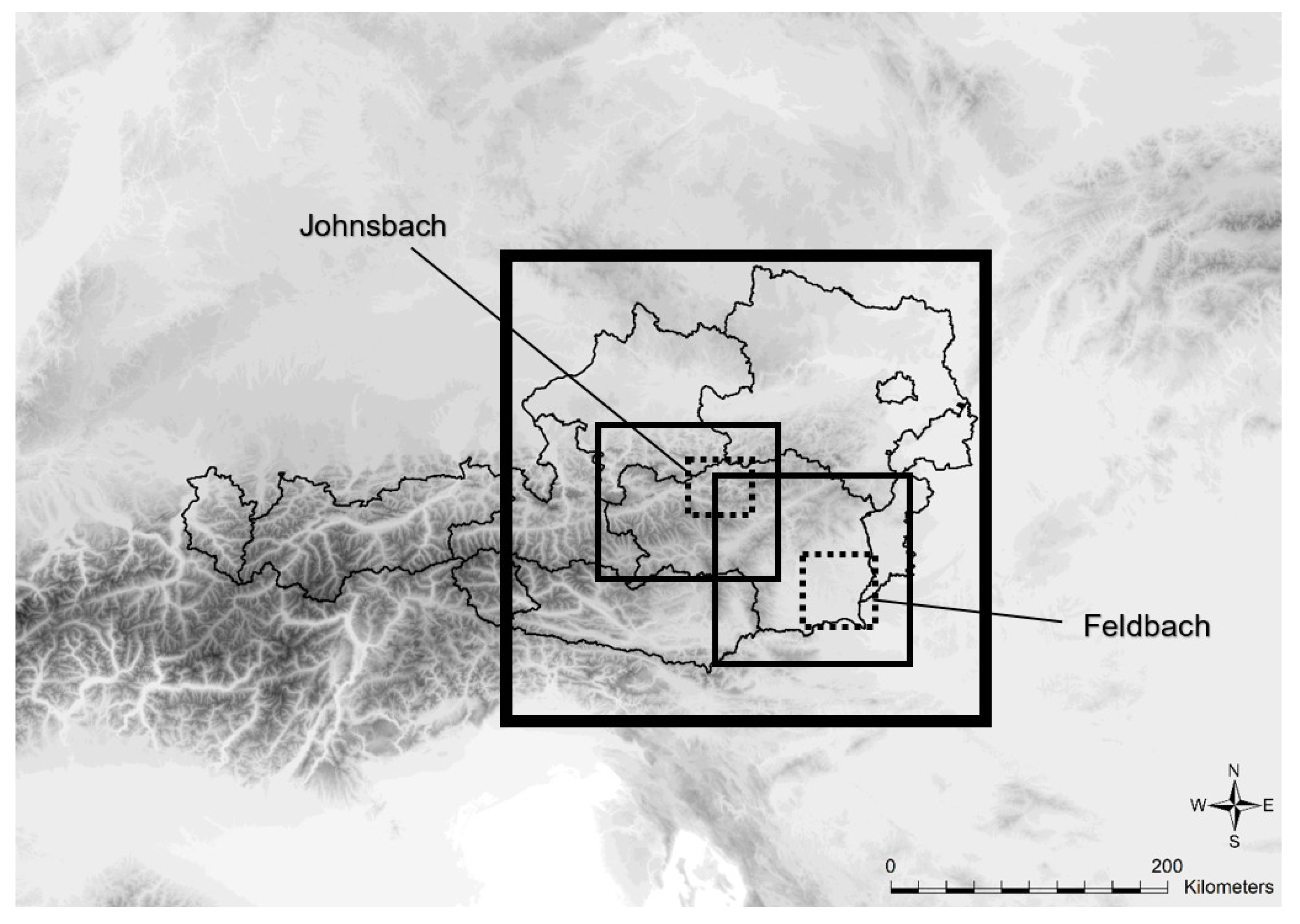
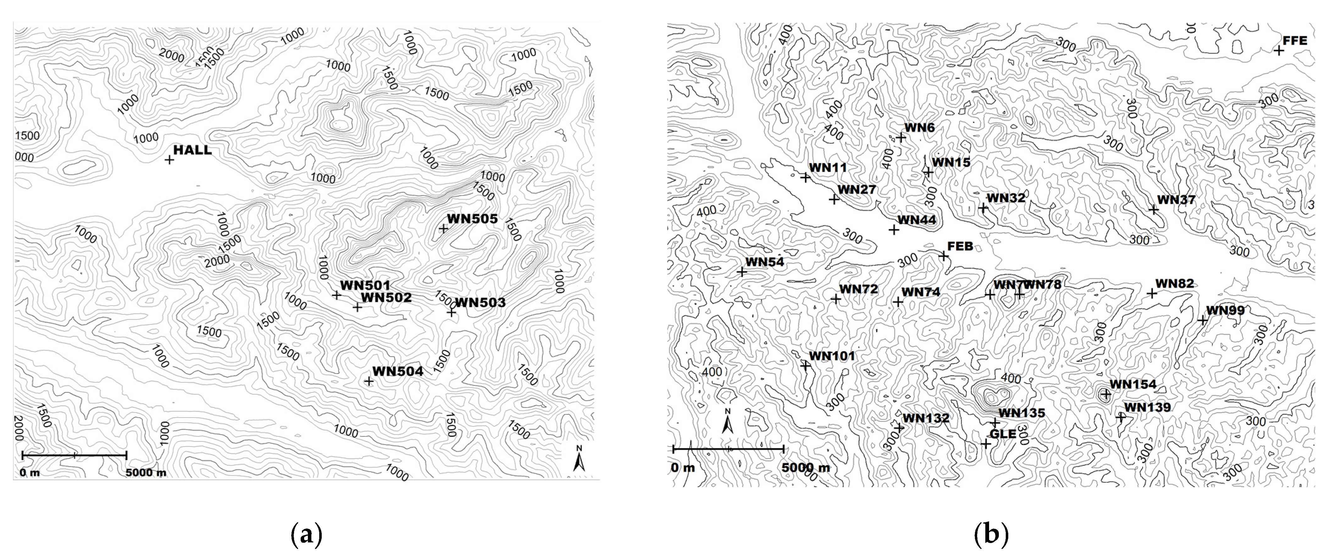
3. Study Area
4. Results
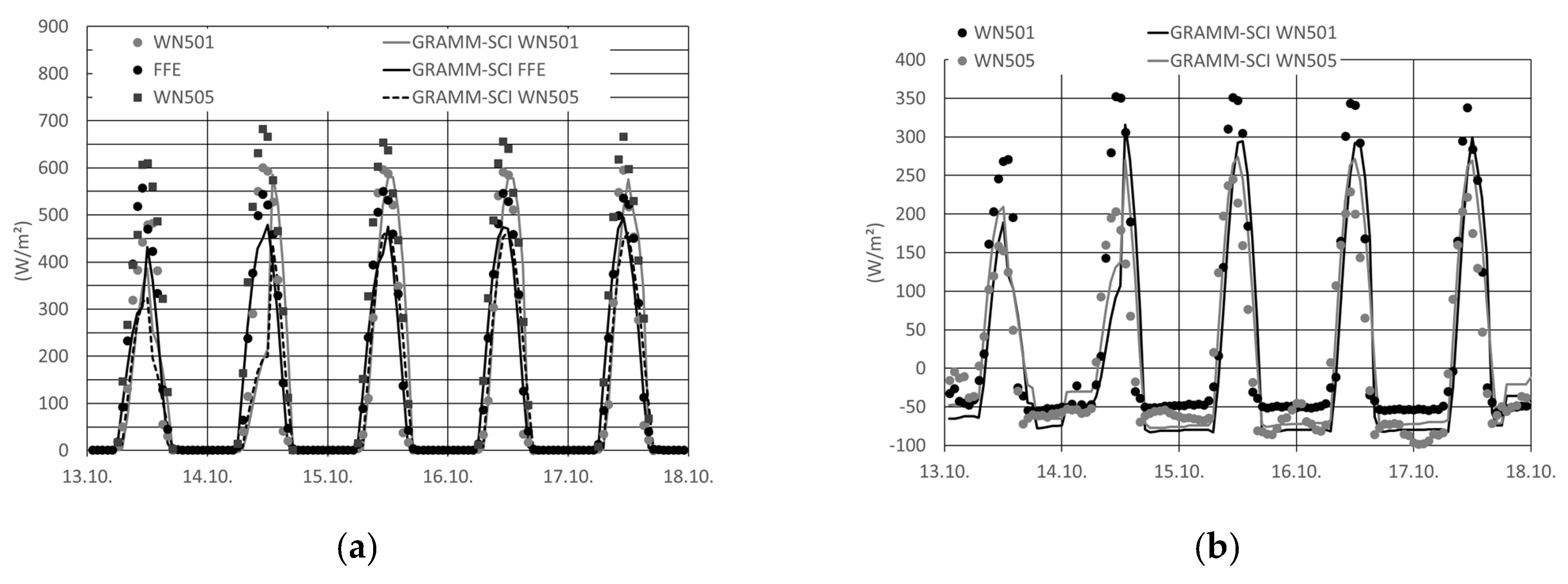
4.1. Radiation
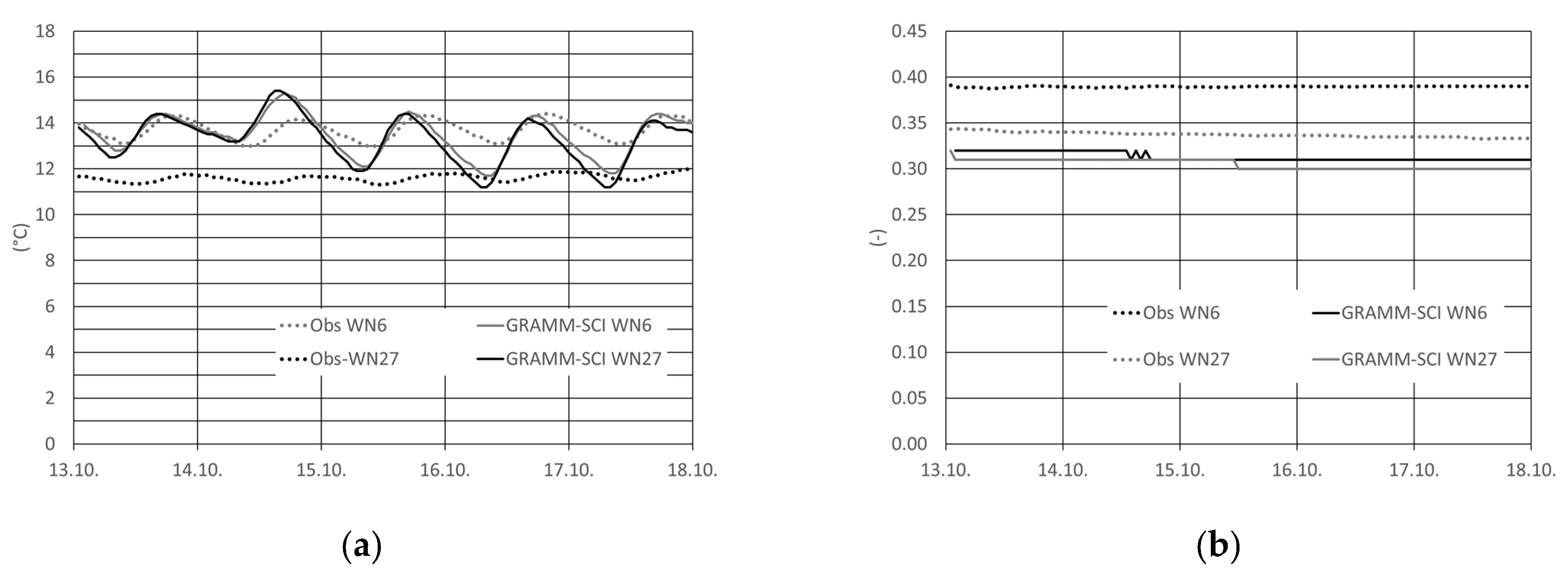
4.2. Soil Temperature and Moisture
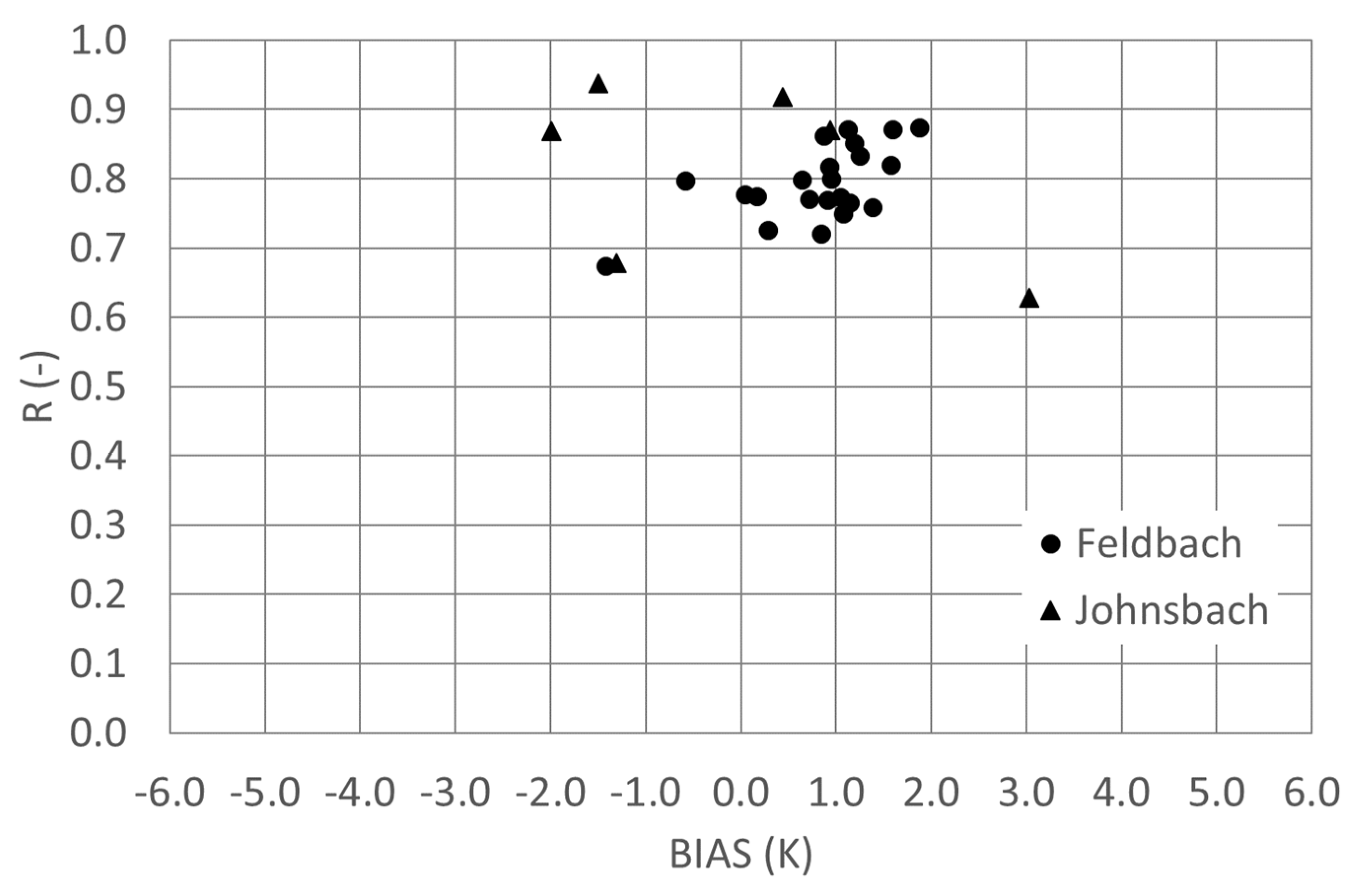
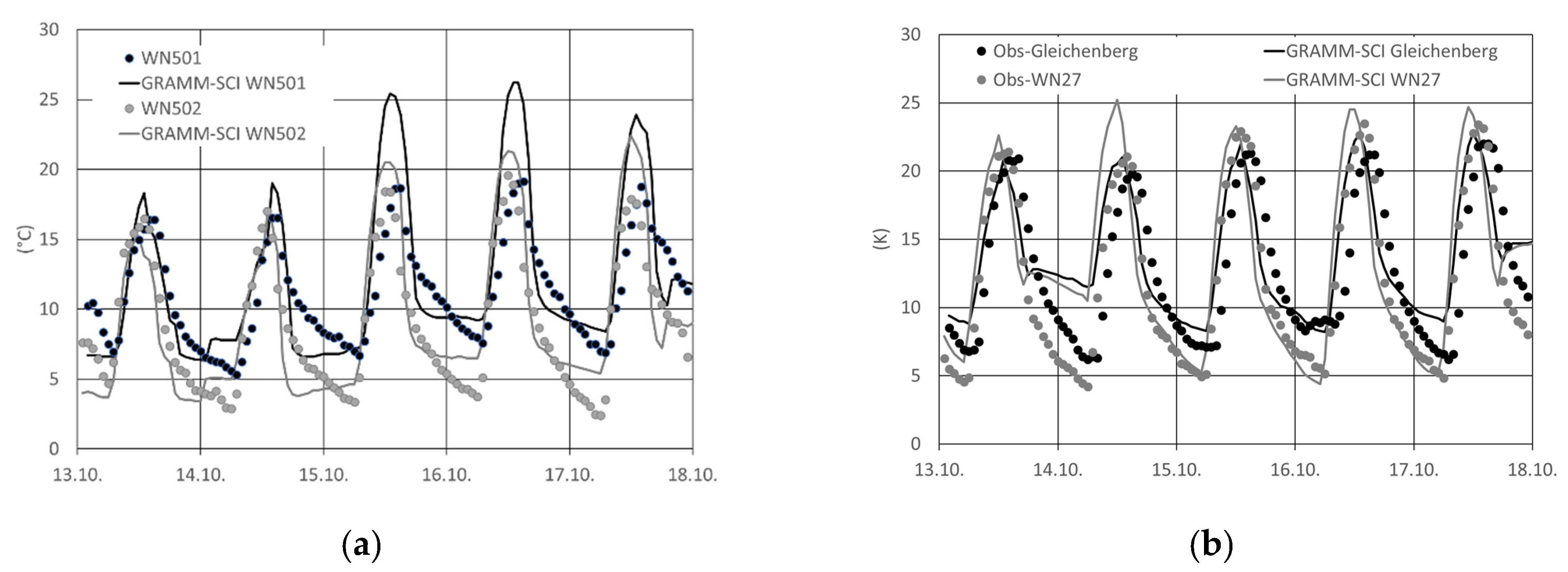
4.3. Air Temperature
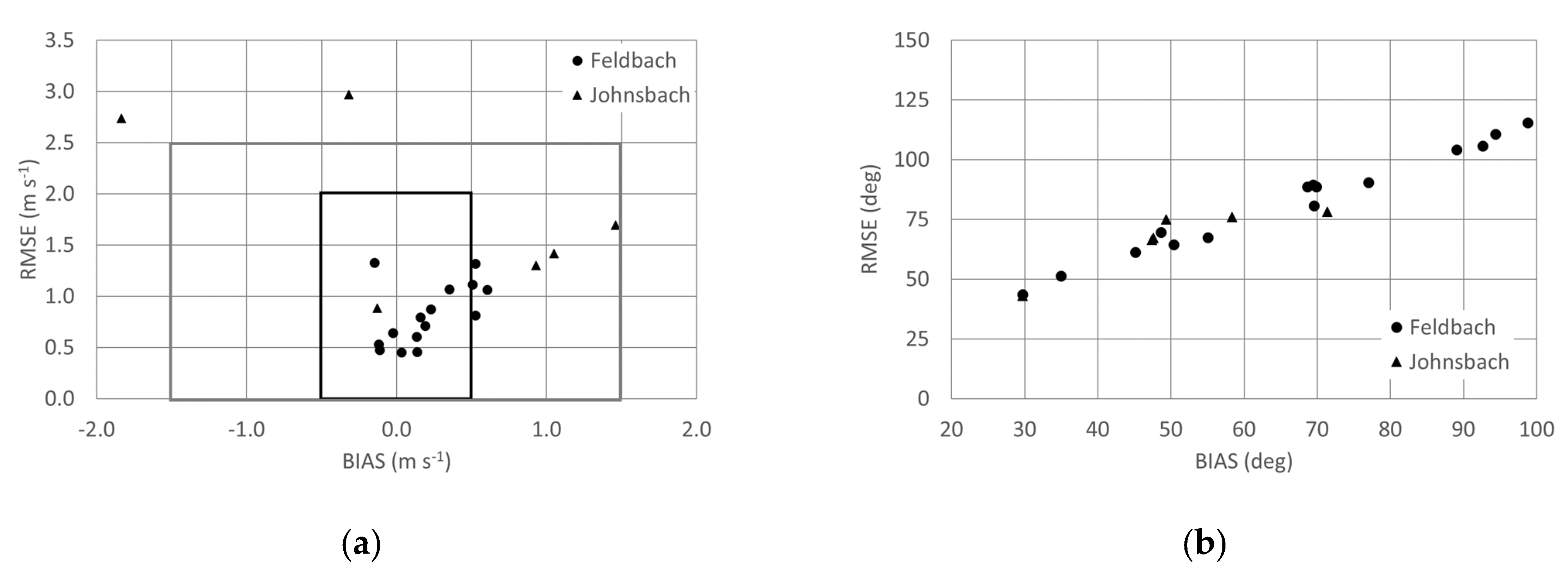
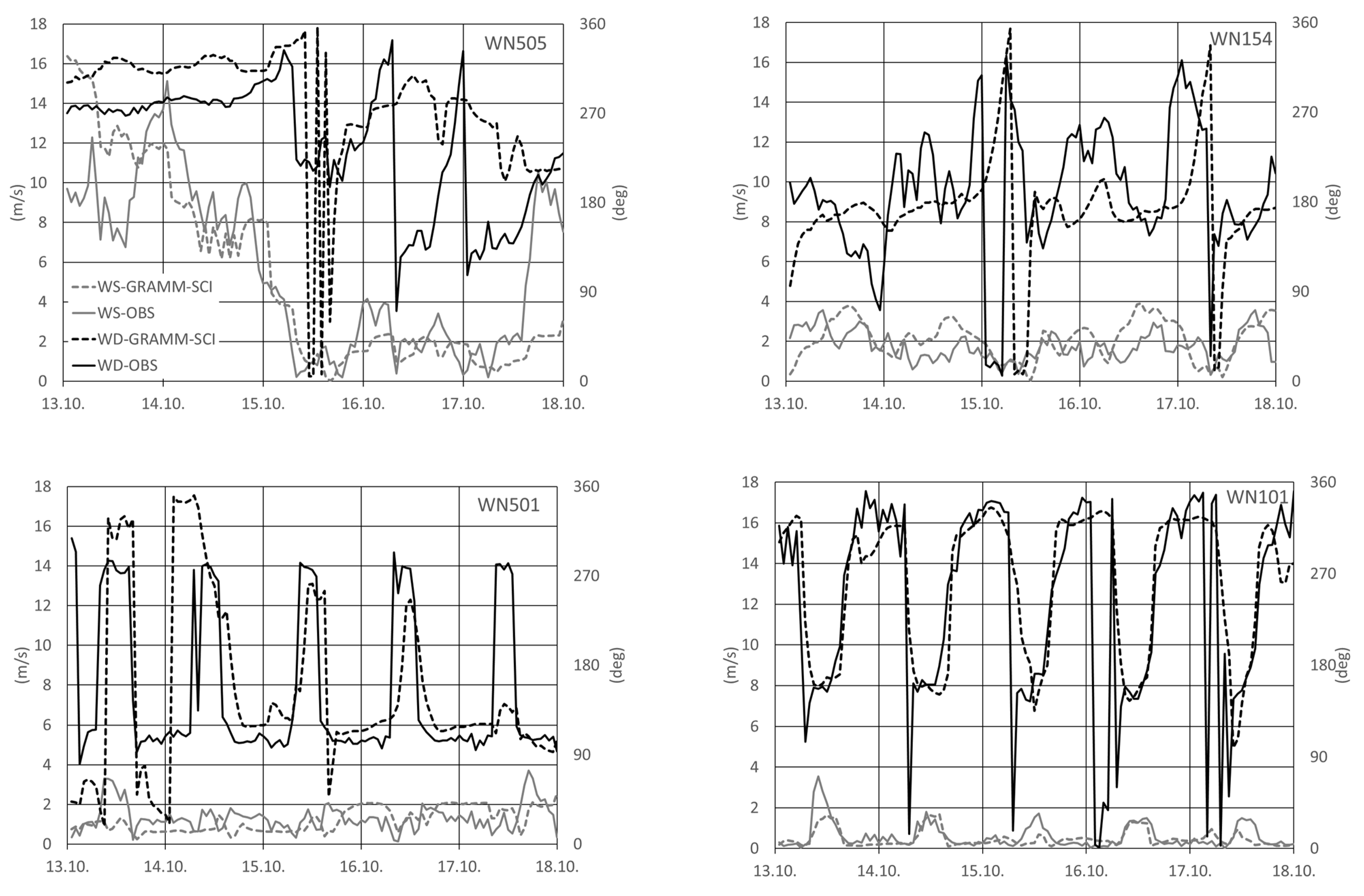
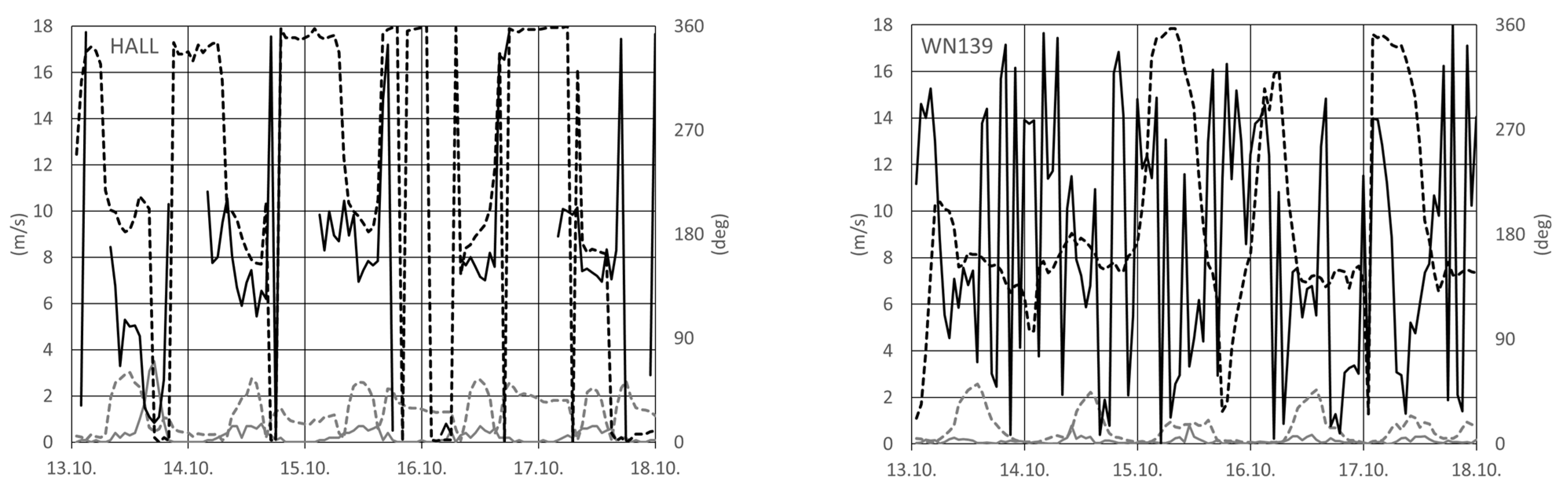
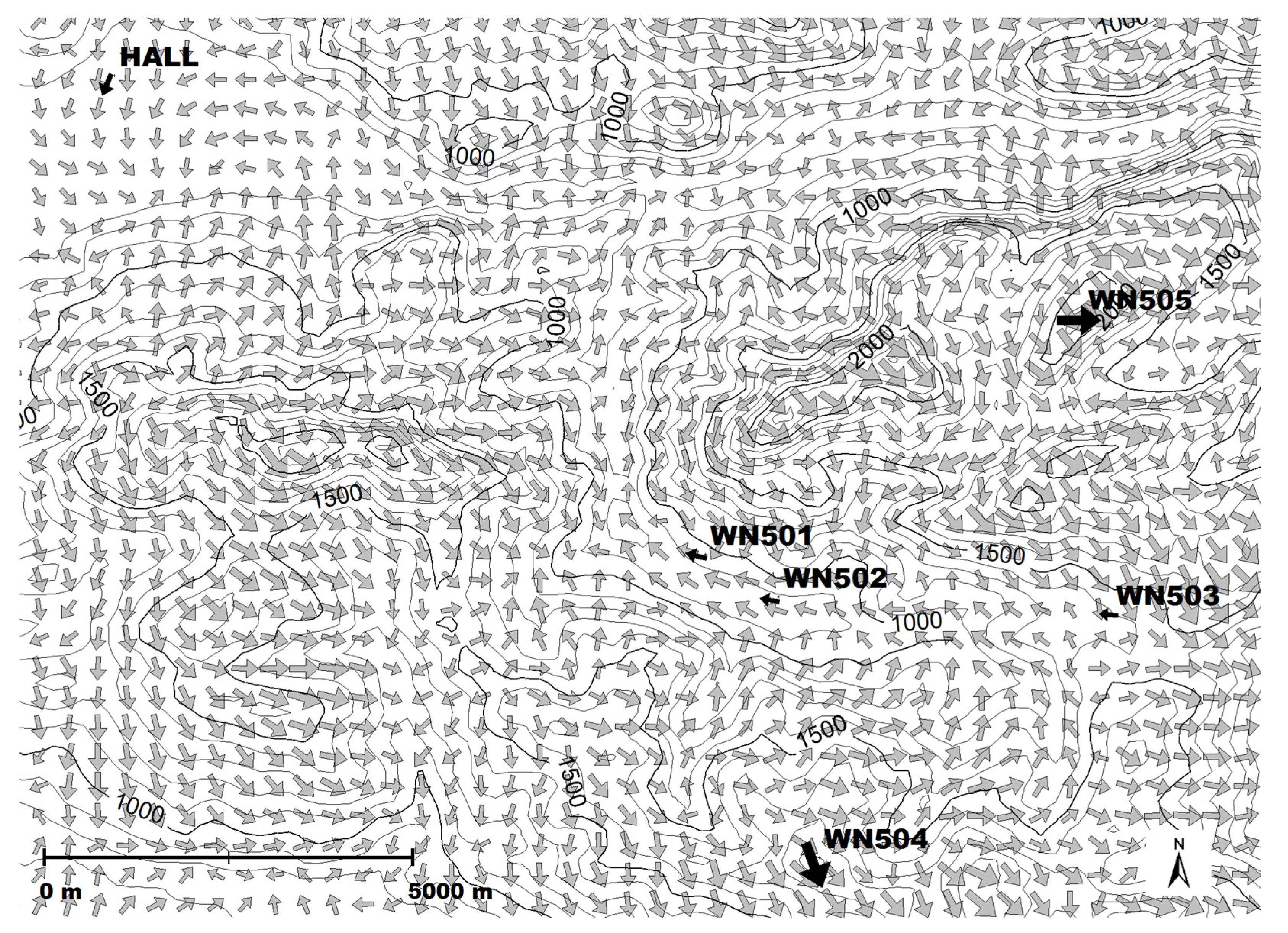
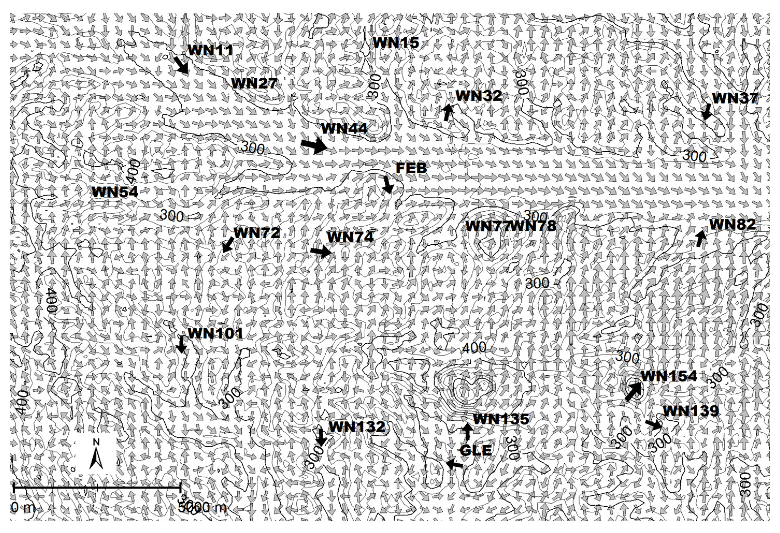
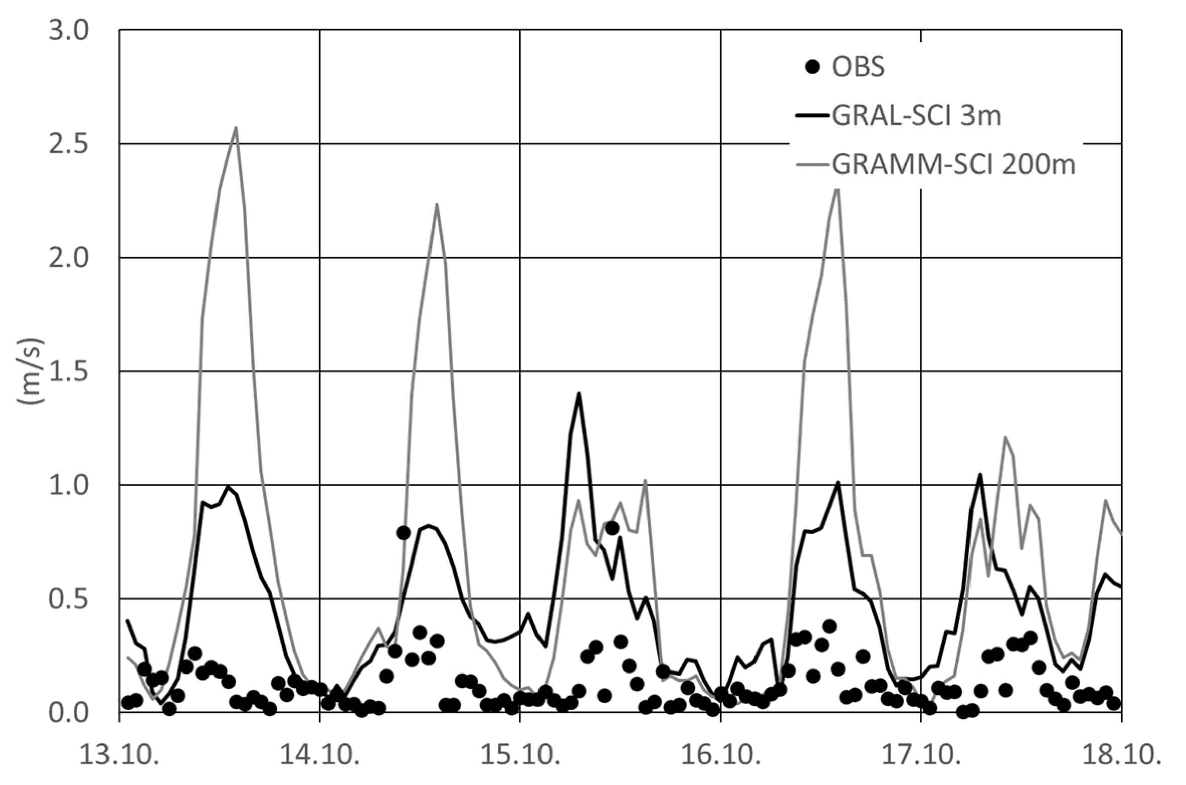
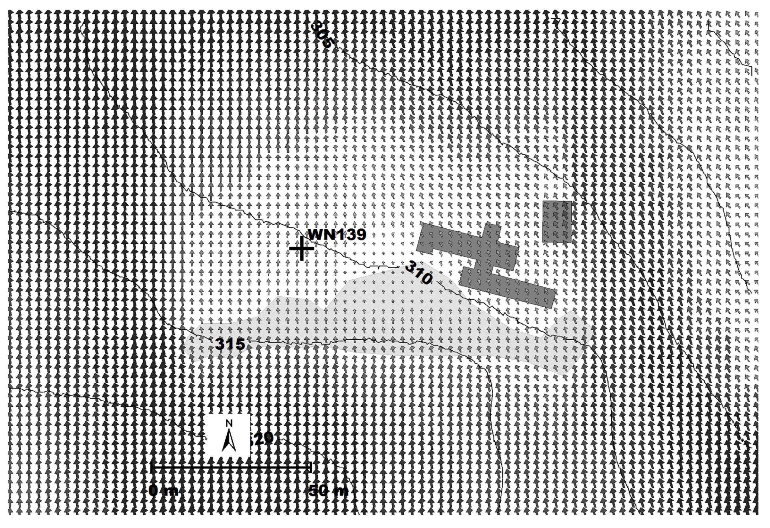
4.4. Wind Speed and Direction
5. Conclusions
Funding
Institutional Review Board Statement
Informed Consent Statement
Data Availability Statement
Conflicts of Interest
References
- Oettl, D. High Resolution Maps of Nitrogen Dioxide for the Province of Styria, Austria. Int. J. Environ. Pollut. 2014, 54, 137–146. [Google Scholar] [CrossRef]
- Berchet, A.; Zink, K.; Müller, C.; Oettl, D.; Brunner, J.; Emmenegger, L.; Brunner, D. A cost-effective method for simulation city-wide air flow and pollutant dispersion at building resolving scale. Atmos. Environ. 2017, 158, 181–196. [Google Scholar] [CrossRef]
- Berchet, A.; Zink, K.; Oettl, D.; Brunner, J.; Emmenegger, L.; Brunner, D. Evaluation of high-resolution GRAMM–GRAL (v15.12/v14.8) NOx simulations over the city of Zürich, Switzerland. Geosci. Model Dev. 2017, 10, 3441–3459. [Google Scholar] [CrossRef]
- Bernhardt, M.; Zängl, G.; Liston, G.E.; Strasser, U.; Mauser, W. Using wind fields from a high-resolution atmospheric model for simulating snow dynamics in mountainous terrain. Hydrol. Process. 2008, 23, 1064–1075. [Google Scholar] [CrossRef]
- Misenis, C.; Thurman, J.; Owen, R.C. Prognostic meteorological data in dispersion applications. In Proceedings of the 19th International Conference on Harmonisation within Atmospheric Dispersion Modelling for Regulatory Purposes, Bruges, Belgium, 3–6 June 2019. [Google Scholar]
- Dörenkämper, M.; Olsen, B.T.; Witha, B.; Hahmann, A.N.; Davis, N.N.; Barcons, J.; Ezber, A.; García-Bustamante, E.; González-Rouco, J.F.; Navarro, J.; et al. The Making of the New European Wind Atlas, Part 2: Production and Evaluation. Geosci. Model Dev. 2020. [Google Scholar] [CrossRef]
- Oettl, D. Evaluierung des nichthydrostatischen mesoskaligen Modells GRAMM-SCI anhand der VDI Richtlinie 3783 Blatt 7. Gefahrst. Reinhalt. Luft 2020, 80, 318–324. [Google Scholar]
- Oettl, D.; Veratti, G. A comparative study of mesoscale flow-field modelling in an Eastern Alpine region using WRF and GRAMM-SCI. Atmos Res. 2021, 249, 105288. [Google Scholar] [CrossRef]
- Copernicus Climate Change Service (C3S). ERA5: Fifth Generation of ECMWF Atmospheric Reanalyses of the Global Climate. Copernicus Climate Change Service Climate Data Store (CDS). 2017. Available online: https://cds.climate.copernicus.eu/cdsapp#!/home (accessed on 18 March 2020).
- Skamarock, W.C.; Klemp, J.B.; Dudhia, J.; Gill, D.O.; Barker, D.M.; Wang, W.; Powers, J.G. A Description of the Advanced Research WRF Version 3; Technical Report, NCAR Technical Note TN-475+STR; National Center for Atmospheric Research: Boulder, CO, USA, 2008; 125p. [Google Scholar]
- Fuchsberger, J.; Kirchengast, G.; Bichler, C.; Leuprecht, A.; Kabas, T. WegenerNet Climate Station Network Level 2 Data Version 7.1 (2007–2019); University of Graz, Wegener Center for Climate and Global Change: Graz, Austria, 2020. [Google Scholar] [CrossRef]
- Schlager, C.; Kirchengast, G.; Fuchsberger, J.; Kann, A.; Truhetz, H. A spatial evaluation of high-resolution wind fields from empirical and dynamical modelling in hilly and mountainous terrain. Geosci. Model Dev. 2018. [Google Scholar] [CrossRef]
- Oettl, D. Documentation of the Prognostic Mesoscale Model GRAMM-SCI (Graz Mesoscale Model—Scientific) Version 21.1; Amt d. Stmk. Landesregierung, ABT15, Referat Luftreinhaltung; Government of Styria: Graz, Austria, 2021; 127p, Available online: https://www.researchgate.net/profile/Dietmar_Oettl/publications (accessed on 24 February 2021).
- Dutton, J.A.; Fichtel, G.H. Approximate equations of motion for gases and liquids. J. Atmos. Sci. 1969, 26, 241–254. [Google Scholar] [CrossRef]
- Pielke, R.A. Mesoscale Meteorological Modeling; Academic Press: London, UK, 1984. [Google Scholar]
- Somieski, F. Mesoscale Model Parameterizations for Radiation and Turbulent Fluxes at the Lower Boundary; Deutsches Luft- und Raumfahrtzentrum Oberpfaffenhofen, Inst. für Nachrichtentechnik und Erkundung, Institut für Physik der Atmosphäre: Oberpfaffenhofen, Germany, 1988; p. 39. [Google Scholar]
- Businger, J.A.; Wyngaard, J.C.; Izumi, Y.; Bradley, E.F. Flux-profile relationships in the atmospheric surface layer. J. Atmos. Sci. 1971, 28, 181–189. [Google Scholar] [CrossRef]
- Horvath, K.; Koracin, D.; Vellore, R.; Jiang, J.; Belu, R. Sub-kilometer dynamical downscaling of near-surface winds in complex terrain using WRF and MM5 mesoscale models. J. Geophys. Res. 2012, 117. [Google Scholar] [CrossRef]
- Oettl, D. Quality assurance of the prognostic, microscale wind-field model GRAL 14.8 using wind-tunnel data provided by the German VDI guideline 3783-9. J. Wind Eng. Ind. Aerodyn. 2015, 142, 104–110. [Google Scholar] [CrossRef]
- Oettl, D. A multiscale modelling methodology applicable for regulatory purposes taking into account effects of complex terrain and buildings on the pollutant dispersion: A case study for an inner Alpine basin. Environ. Sci. Pollut. Res. 2015, 22, 17860–17875. [Google Scholar] [CrossRef] [PubMed]
- Schmid, F.; Schmidli, J.; Hervo, M.; Haefele, A. Diurnal Valley Winds in a Deep Alpine Valley: Observations. Atmosphere 2020, 11, 54. [Google Scholar] [CrossRef]
- Zardi, D.; Whiteman, C.D. Diurnal Mountain Wind Systems. Mountain Weather Research and Forecasting; Chow, F.K., DeWekker, S.F.J., Snyder, B., Eds.; Springer: Dordrecht, The Netherlands, 2012. [Google Scholar]
- ZAMG. Weather Map of Europe. 2021. Available online: https://www.zamg.ac.at/cms/de/wetter/wetterkarte (accessed on 24 February 2021).
- Giovannini, L.; Zardi, D.; de Franceschi, M.; Chen, F. Numerical simulations of boundary-layer processes and urban-induced alterations in an Alpine valley. Int. J. Climatol. 2014, 34, 1111–1131. [Google Scholar] [CrossRef]
- Gsella, A.; de Mejij, A.; Kerschbaumer, A.; Reimer, E.; Thunis, P.; Cuvelier, C. Evaluation of MM5, WRF and TAMPER meteorology over the complex terrain of the Po Valley, Italy. Atmos. Environ. 2014, 89, 797–806. [Google Scholar] [CrossRef]
- Schmidli, J.; Böing, S.; Fuhrer, O. Accuracy of Simulated Diurnal Valley Winds in the Swiss Alps: Influence of Grid Resolution, Topography Filtering, and Land Surface Datasets. Atmosphere 2018, 9, 196. [Google Scholar] [CrossRef]
- Veratti, G.; Fabbi, S.; Bigi, A.; Lupascu, A.; Tinarelli, G.; Teggi, S.; Brusasca, G.; Butler, T.M.; Ghermandi, G. Towards the coupling of a chemical transport model with a micro-scale Lagrangian modelling system for evaluation of urban levels in a European hotspot. Atmos. Environ. 2020, 223, 117285. [Google Scholar] [CrossRef]
- Schlager, C.; Kirchengast, G.; Fuchsberger, J. Empirical high-resolution wind field and gust model in mountainous and hilly terrain based on the dense WegenerNet station networks. Atmos. Meas. Tech. 2018, 11, 5607–5627. [Google Scholar] [CrossRef]
- Haiden, T.; Kann, A.; Wittmann, C.; Pistotnik, G.; Bica, B.; Gruber, C. The Integrated Nowcasting through Comprehensive Analysis (INCA) system and its validation over the eastern alpine region. Weather Forecast. 2011, 26, 166–183. [Google Scholar] [CrossRef]
- Wang, Y.; Haiden, T.; Kann, A. The Operational Limited Area Modelling System at ZAMG: ALADIN-AUSTRIA; 37; Österreichische Beiträge zu Meteorologie und Geophysik: Vienna, Austria, 2006. [Google Scholar]
- Schaettler, G.D.; Baldauf, M. A Description of the Nonhydrostatic Regional COSMO Model; Part VII: User’s Guide; Deutscher Wetterdienst: Offenbach, Germany, 2016. [Google Scholar]
- EEA. The Application of Models under the European Union’s Air Quality Directive: A Technical Reference Guide; Technical Report 10/2011; European Environmental Agency: Copenhagen, Denmark, 2011; 90p. [Google Scholar] [CrossRef]
- Cantelli, A.; Monti, P.; Leuzzi, G.; Valerio, G.; Pilotti, M. Numerical simulations of mountain winds in an alpine valley. Wind Struct. 2017, 24, 565–578. [Google Scholar]
- Schluenzen, H.; Conrady, K.; Purr, C. Typical performances of mesoscale meteorology models. In Proceedings of the 34th International Technical Meeting on Air Pollution Modelling and its Application, Montpellier, France, 4–8 May 2015; 8p. [Google Scholar]
- De Meij, A.; Gzella, A.; Cuvelier, C.; Thunis, P.; Bessagnet, B.; Vinuesa, J.F.; Menut, L.; Kelder, H.M. The impact of MM5 and WRF meteorology over complex terrain on CHIMERE model calculations. Atmos. Chem. Phys. 2009, 9, 6611–6632. [Google Scholar] [CrossRef]
- Goger, B.; Rotach, M.W.; Gohm, A.; Fuhrer, O.; Stiperski, I.; Holtslag, A.A.M. The Impact of Three-Dimensional Effects on the Simulation of Turbulence Kinetic Energy in a Major Alpine Valley. Bound. Layer Meterol. 2018, 168, 1–27. [Google Scholar] [CrossRef] [PubMed]
- Mahrt, L. Microfronts in the nocturnal boundary layer. Q. J. R. Meteorol. Soc. 2019, 145, 546–562. [Google Scholar] [CrossRef]
- Oettl, D. Documentation of the Lagrangian Particle Model GRAL-SCI (Graz Lagrangian Model—Scientific) Version 21.1; Amt d. Stmk. Landesregierung, ABT15, Referat Luftreinhaltung; Government of Styria: Graz, Austria, 2021; 202p, Available online: https://www.researchgate.net/profile/Dietmar_Oettl/publications (accessed on 24 February 2021).
- Amiro, B.D. Comparison of turbulence statistics within three boreal forest canopies. Bound. Layer Meteorol. 1990, 51, 99–121. [Google Scholar] [CrossRef]


| Code | Description | Albedo [-] | Emissivity [-] | Roughness Length [m] | Heat Conductivity [W/m/K] | Thermal Diffusivity [m²/s] |
|---|---|---|---|---|---|---|
| 111 | Continuous urban fabric | 0.25 | 0.95 | 1 | 1 | 2.0 × 10⁻⁶ |
| 112 | Discontinuous urban fabric | 0.25 | 0.95 | 0.5 | 1 | 1.3 × 10⁻⁶ |
| 211 | Non-irrigated arable land | 0.19 | 0.92 | 0.1 | 0.2 | 7.0 × 10⁻⁷ |
| 231 | Pastures | 0.19 | 0.92 | 0.1 | 0.2 | 7.0 × 10⁻⁷ |
| 241 | Annual crops associated with permanent crops | 0.19 | 0.92 | 0.1 | 0.2 | 7.0 × 10⁻⁷ |
| 243 | Land principally occupied by agriculture, with significant areas of natural vegetation | 0.19 | 0.92 | 0.2 | 0.2 | 7.0 × 10⁻⁷ |
| 311 | Broad-leaved forest | 0.16 | 0.90 | 1 | 0.2 | 8.0 × 10⁻⁷ |
| 312 | Coniferous forest | 0.12 | 0.90 | 1 | 0.2 | 8.0 × 10⁻⁷ |
| 313 | Mixed forest | 0.14 | 0.90 | 1 | 0.2 | 8.0 × 10⁻⁷ |
| 321 | Natural grasslands | 0.15 | 0.92 | 0.02 | 0.2 | 1.0 × 10⁻⁶ |
| 332 | Bare rocks | 0.15 | 0.92 | 0.1 | 1 | 1.0 × 10⁻⁶ |
| 511 | Water courses | 0.08 | 0.98 | 0.0001 | 100 | 1.0 × 10⁻⁶ |
| Station | Longitude (°) | Latitude (°) | Altitude (m) | Parameters | Wind Sensor Height above Ground (m) |
|---|---|---|---|---|---|
| GLEICHENBERG (GLE) | 15.90361 | 46.87222 | 269 | u, Tair | 18 |
| FELDBACH (FEB) | 15.87972 | 46.94889 | 323 | u, Tair | 10 |
| FUERSTENFELD (FFE) | 16.08083 | 47.03083 | 271 | u, Tair, rglob | 10 |
| WN6 | 15.85507 | 46.99726 | 398 | Tsoil, Msoil | - |
| WN11 | 15.79801 | 46.98137 | 300 | u, Tair | 10 |
| WN15 | 15.87115 | 46.98299 | 297 | Tsoil, Msoil | - |
| WN27 | 15.81499 | 46.97232 | 298 | Tsoil, Msoil | - |
| WN44 | 15.85036 | 46.95979 | 288 | u, Tair | 55 |
| WN54 | 15.75960 | 46.94327 | 348 | Tsoil, Msoil | - |
| WN72 | 15.81543 | 46.93182 | 337 | u, Tair | 18 |
| WN77 | 15.90706 | 46.93294 | 306 | Tsoil, Msoil | - |
| WN78 | 15.92462 | 46.93291 | 372 | Tsoil, Msoil | - |
| WN82 | 16.00336 | 46.93263 | 276 | u, Tair | 10 |
| WN99 | 16.03337 | 46.92135 | 270 | Tsoil, Msoil | - |
| WN101 | 15.79682 | 46.90473 | 304 | u, Tair | 14 |
| WN132 | 15.85215 | 46.87902 | 295 | u, Tair | 10 |
| WN139 | 15.98394 | 46.88229 | 307 | u, Tair | 10 |
| WN154 | 15.97547 | 46.89181 | 471 | u, Tair | 10 |
| HALL | 14.49083 | 47.59472 | 637 | u, Tair | 10 |
| WN501 | 14.59800 | 47.53640 | 920 | u, Tair, rnet, rglob | 10 |
| WN502 | 14.61130 | 47.53120 | 860 | u, Tair, rnet, rglob | 10 |
| WN503 | 14.67132 | 47.52922 | 1344 | u, Tair, rnet, rglob | 10 |
| WN504 | 14.61885 | 47.49936 | 1969 | u, Tair, rnet, rglob | 6 |
| WN505 | 14.66605 | 47.56540 | 2191 | u, Tair, rnet, rglob | 6 |
| BIAS | RMSE | R | Hit Rates | ||||||
|---|---|---|---|---|---|---|---|---|---|
| u (m s−1) | Θ (deg) | u (m s−1) | Θ (deg) | u (-) | Θ (-) | u (-) | Θ (-) | ||
| ERA5 | Johnsbach | 1.21 | 74 | 2.04 | 87 | 0.40 | 0.36 | 0.0 | 0.33 |
| Feldbach | 0.82 | 80 | 1.23 | 94 | 0.32 | 0.17 | 0.2 | 0.67 | |
| 1000 m | Johnsbach | 2.01 | 60 | 2.77 | 76 | 0.27 | 0.22 | 0.0 | 0.50 |
| Feldbach | 0.25 | 73 | 0.79 | 88 | 0.25 | 0.19 | 0.93 | 0.67 | |
| 200 m | Johnsbach | 0.95 | 51 | 1.83 | 68 | 0.36 | 0.45 | 0.17 | 0.67 |
| Feldbach | 0.25 | 66 | 0.82 | 82 | 0.32 | 0.20 | 0.73 | 0.80 | |
Publisher’s Note: MDPI stays neutral with regard to jurisdictional claims in published maps and institutional affiliations. |
© 2021 by the author. Licensee MDPI, Basel, Switzerland. This article is an open access article distributed under the terms and conditions of the Creative Commons Attribution (CC BY) license (http://creativecommons.org/licenses/by/4.0/).
Share and Cite
Oettl, D. Development of the Mesoscale Model GRAMM-SCI: Evaluation of Simulated Highly-Resolved Flow Fields in an Alpine and Pre-Alpine Region. Atmosphere 2021, 12, 298. https://doi.org/10.3390/atmos12030298
Oettl D. Development of the Mesoscale Model GRAMM-SCI: Evaluation of Simulated Highly-Resolved Flow Fields in an Alpine and Pre-Alpine Region. Atmosphere. 2021; 12(3):298. https://doi.org/10.3390/atmos12030298
Chicago/Turabian StyleOettl, Dietmar. 2021. "Development of the Mesoscale Model GRAMM-SCI: Evaluation of Simulated Highly-Resolved Flow Fields in an Alpine and Pre-Alpine Region" Atmosphere 12, no. 3: 298. https://doi.org/10.3390/atmos12030298
APA StyleOettl, D. (2021). Development of the Mesoscale Model GRAMM-SCI: Evaluation of Simulated Highly-Resolved Flow Fields in an Alpine and Pre-Alpine Region. Atmosphere, 12(3), 298. https://doi.org/10.3390/atmos12030298