Article

Characteristics of Energy Dissipation Rate Observed from the High-Frequency Sonic Anemometer at Boseong, South Korea

1
School of Earth and Environmental Sciences, Seoul National University, Seoul 08826, Korea
2
National Center for Atmospheric Research, Research Application Laboratory, Boulder, CO 80307, USA
*
Author to whom correspondence should be addressed.
Atmosphere 2021, 12(7), 837; https://doi.org/10.3390/atmos12070837
Submission received: 10 June 2021 / Accepted: 24 June 2021 / Published: 29 June 2021
(This article belongs to the Special Issue Low Level Windshear and Turbulence for Aviation Safety)

Abstract

:
The characteristics of low-level turbulence at Boseong, located on the southern coast of South Korea, were investigated in terms of eddy dissipation rate (EDR) using 1-year (2018) of wind data obtained from the Boseong Meteorological Observatory (BMO), a World Meteorological Organization testbed. At BMO, a 307 m tall tower is installed on which four high-frequency (20 Hz) sonic anemometers are mounted at 60, 140, and 300 m above ground level (AGL). In addition, a sonic anemometer at 2.5 m AGL is located to the south of the tower. EDRs are estimated from the wind measurements based on three different EDR estimation methods. The first two methods use the inertial dissipation method derived from Kolmogorov turbulence theory, and the third uses a maximum likelihood estimation assuming a von Kármán spectral model. Reasonable agreement was obtained between the three methods with various fluctuations, including diurnal variations for all seasons, while the EDR calculated from the third method displayed slightly higher EDR values than the other two methods. The result of the analysis showed that the mean (standard deviations) of logarithms of EDR had larger values as height decreased (increased), and the means were higher in the unstable planetary boundary layer (PBL) than in the stable PBL for this heterogeneous location adjacent to the coastlines. The probability density functions (PDFs) of the EDRs showed that the distribution was well-represented by a lognormal distribution in both the stable and unstable PBL, although the PDFs at the lowest level (2.5 m) deviated from those at other levels due to surface effects. Seasonal variations in the PDFs showed that there was less difference in the shape of the PDFs depending on atmospheric stability in the wintertime. Finally, we calculate the 1-yr statistics of the observed EDR, which will be used for future LLT forecast systems in Korea.

1. Introduction

The energy (or eddy) dissipation rate ( ε ) is the rate at which turbulent kinetic energy (TKE) cascades down to smaller scales. The cube root of the turbulence dissipation rate ( ε 1 / 3 ) is frequently used in the field of aviation turbulence meteorology since it is proportional to aircraft loads [1]. This quantity is termed as energy or eddy dissipation rate to the one-third power (EDR) and is regarded as the standard metric for reporting turbulence intensity by the International Civil Aviation Organization (ICAO) [2]. Turbulence dissipation rate in the atmospheric boundary layer (i.e., planetary boundary layer; PBL) has been the subject of many investigations, including the effect on the frontogenesis [3], in the evaluations of the PBL parameterizations [4], in the energy production from the wind farms [5], and in the development of low-level turbulence (LLT) forecasting systems [6]. These and other studies have been based on sonic anemometer data [3,4,5,6,7,8], aircraft data [9,10,11], lidars [7,12,13,14,15,16,17], and radars [10,18,19].
Most previous studies show that the observed behavior of the EDR follows a lognormal distribution in the free atmosphere, which is typically stably stratified [9,20]. Based on the lognormality observed in the commercial aircraft in-situ EDR observations, the lognormal mapping technique (LMT) has been recently used in the development of numerical weather prediction (NWP) model-based turbulence forecast systems such as the Graphical Turbulence Guidance (GTG) [21,22]. In the GTG system, multiple turbulence diagnostics based on various empirical and physical methods are calculated from a collection of meteorological variables and their horizontal or vertical gradients. Then, those are converted into EDR forecasts by the LMT scheme assuming these variables follow lognormal distributions. LMT requires the observed climatological statistics (mean and standard deviations) of the logarithms of the EDRs. Such values were calculated for various altitudes of the atmosphere by the EDR estimation methods based on the inertial dissipation method (IDM) and von Kármán spectral model [9]. Using this, the GTG systems targeting global and regional domains have been developed based on the NWP model outputs [21,22]. These systems mainly focused on the forecasts of clear-air turbulence (CAT) and mountain-wave turbulence but now provide LLT forecasts as well [6].
Previous studies have shown the probability density function (PDF) of EDR exhibits a pronounced diurnal variation following the temporal evolution of the PBL [4]. The PDFs were also observed to have different shapes during the day and night [4]. Specifically, the PDF approximates a lognormal distribution:
PDF ( ln x ) = 1 2 π σ 2 exp ( ln x μ 2 σ 2 )
in the nighttime stable PBL and a log-Weibull distribution
PDF ( ln x ) = k λ ( ln x λ ) k 1 exp { ( ln x λ ) k }
in the daytime unstable PBL. These characteristics are found from measurements during the eXperimental Planetary boundary layer Instrumentation Assessment (XPIA) field campaign, held at Boulder, Colorado [23]. Based on these observations, an improved LLT forecasting system was developed using the statistics derived from the lognormal and the log-Weibull distributions of the observed EDRs [6]. However, it is expected that this behavior is geographically dependent, so in order to implement LLT forecasting systems globally, further investigations of the PDFs of observed EDR in the PBL outside Boulder are required.
The characteristics of turbulence dissipation rate (ε) were also explored at other locations more heterogeneous than the Boulder site, which is relatively flat and is located in the middle of the continental United States. For example, the characteristics of ε were investigated during a Bora event using sonic anemometer measurements [8]. It was found that a power law can be established empirically between the mean wind speed and ε. During the second Wind Forecast Improvement Project (WFIP2) field campaign [24], the variability of ε was observed over complex terrain using various atmospheric measurement instruments such as lidars and anemometers [15]. It was shown that the leeside wind increased the turbulence production and ε, and ε was larger in the summertime than in the wintertime due to increased convective mixing. Furthermore, the dependence of wind direction on ε was analyzed in an offshore area using lidar measurements [16]. It was suggested that the wind from the open ocean interacted with the relatively lower surface roughness of the ocean, and therefore generated less TKE and ε, compared to instances when the wind was from the land. In addition, it was reported that the ε was higher in wintertime than in summertime because the wind from the land to the ocean was more frequent in wintertime and vice versa. Overall, the above studies indicate that the characteristics of ε or EDR are strongly affected by geographic location, and thus, various aspects of these characteristics can be expected in different locations.
In this study, the sonic anemometer wind measurements at BMO located on the southern coast of South Korea were used to derive seasonal profiles of EDR. The heterogeneity of the terrain and the coastal environment are likely to affect the measurements, considering the location of the BMO (Figure 1). The physical mechanisms mentioned above are likely to occur due to the heterogeneity introduced by the close proximity of mountains to the north and the ocean to the south. This is a unique environment compared to those in previous studies (e.g., [6,7,8]). Hereafter, we emphasize the characteristics of LLT relevant to aviation turbulence. As a consequence, all analyses are conducted and presented in terms of EDR rather than turbulence dissipation rate (ε). Section 2 introduces the data used in this study. Section 3 describes three methods to estimate EDR and briefly examines the validity of each method. Section 4 presents the time series and the statistical properties of EDRs derived from the three different EDR estimation methods. The properties of the PDFs corresponding to seasons and atmospheric stability are discussed in this section, and an example of the development of a low-level forecasting system based on LMT is also suggested in Section 4. Section 5 summarizes the study and proposes future plans for this work.

2. Data

BMO is a testbed of the World Meteorological Organization-Commission for Instruments and Methods of Observation with its purpose of the integration of a 3D weather observation system (https://community.wmo.int/activity-areas/imop/cimo-testbeds-and-lead-centres/Testbed_Korea accessed on 15 May 2021). BMO is a regular observation site operated by the National Institute of Meteorological Sciences (NIMS) of the Korean Meteorological Administration (KMA) in Korea. It has provided long-term atmospheric measurements since 2014. BMO is located at 34.76° N and 127.21° E. The specific location of BMO is displayed in Figure 1 with terrain height overlaid. The southern coastline of the Korean peninsula is adjacent to BMO to the southeast, and some hills and mountains with a maximum height of 576 m are located north to northwest. Although the vicinity of BMO is relatively flat, the complexity of terrain implies that there is strong horizontal surface heterogeneity upstream of BMO. Here, the effects of the marine boundary layer, the mesoscale forcing such as land-sea breeze, and the acceleration of wind in the leeside of the mountains, are expected to affect the characteristics of the observed turbulence.
BMO has a tower on which various atmospheric measurement instruments are installed. Figure 2 shows the bird’s eye view taken by an unmanned air mobility vehicle, and the 307 m meteorological tower established at BMO. Three 3D sonic anemometers (product name: Campbell CSAT3A) are mounted on the tower and are located at 60 m, 140 m, and 300 m above the ground on the northeastern side of the observation boom. In addition, a 3D sonic anemometer is installed at 2.5 m above the ground on a mast located south of the tower (Figure 2). The 3D sonic anemometer measures the 3D components of wind velocity, namely streamwise, transverse, and vertical components of wind velocity, with a 20 Hz sampling rate. For the tower data, we use the raw data provided by the NIMS, which were collected by Campbell LoggerNet software. This includes the 3D components of wind velocity with a 20 Hz sampling rate and 30-min average values of temperature and turbulent quantities such as friction velocity and kinematic heat flux. A 5 m observation boom is installed from the body of the mast for each anemometer level, with each anemometer mounted at the tip of the boom, i.e., 5 m from the body of the mast. Wake effects are considered minimal since the dominant wind direction usually places the anemometers upstream of the mast (This will be shown in Figure 7). The double rotation sonic tilt correction algorithm [25] was tested, and the effect on the shape of the PDFs of EDR (This will be shown in Figure 9) was negligible because the BMO tower is located in a flat area (Figure 1 and Figure 2). For this reason, we did not use the sonic tilt correction algorithm in the analysis. Precipitation records from the automated surface observing system (ASOS) at Boseong (Figure 2) were used to exclude spurious measurements of the anemometers that may have occurred due to the precipitation.
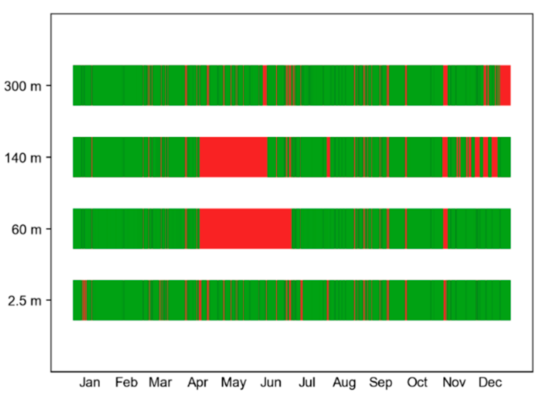
Finally, one year (January to December 2018) of the streamwise component of wind velocity at the four levels was analyzed. The streamwise component was used for two reasons: (1) Most previous investigations of ε used the streamwise component only, so we can compare our results to others, and (2) It is reported that CSAT3 underestimates the vertical component of wind velocity [26]. For the measuring errors of sonic anemometers, most literature mainly adopted methodologies of (1) intercomparisons of different sonic anemometers [27], (2) wind-tunnel experiments [28], and (3) numerical simulations [29]. In terms of estimation errors of EDR, it is possible to perform intercomparisons of EDR from sonic anemometers with indirect estimation (Section 3.1 and Section 3.2) and from hot-wire anemometers with direct estimation [3]. Investigations such as the effect of measuring errors on the estimation of EDR are beyond the scope, and error analysis was not conducted in this research. Some time periods were not available due mainly to routine calibration correction, inspection, and replacement. In addition, the data logger software may raise issues in collecting observation data. These missing measurements were typically concentrated during April, May, and June at 60 m and 140 m. After producing EDRs from the methods described in Section 3, the missing portion of the total amount of EDR was 9.194%, 26.19%, 27.30%, and 12.60% at 2.5 m, 60 m, 140 m, and 300 m, respectively. Figure 3 visualizes the periods of the available and the missing portions of produced EDR at the four levels. The portions of the missing values of EDR in the winter (December, January, and February 2018; DJF), in the spring (March, April, and May 2018; MAM), in the summer (June, July, and August 2018; JJA), and in the fall (September, October, and November 2018; SON) are presented in Table 1.

3. Methodology

The anemometers produce a time series of wind velocities at a fixed location. To adopt the mathematical turbulence models defined in the spatial dimension, it is necessary to invoke Taylor’s frozen hypothesis to bridge the relationship between the physical variables in the spatial (wavenumber) domain and in the time (frequency) domain [30]. Assuming Taylor’s frozen hypothesis,
r = U τ
k = 2 π f U
S ( f ) = 2 π U F ( k )
is approximately valid, where r is spatial separation, U is mean streamwise wind speed, τ is temporal separation, k is the horizontal wavenumber, f is frequency, S ( f ) is the power spectral density (PSD) in the temporal domain, and F ( k ) is the PSD in the spatial domain. Taylor’s frozen hypothesis is valid if the scale of the fluctuation velocity is much smaller than the mean horizontal velocity:
u U 1
where u is the fluctuation velocity [28]. Although this criterion has some limitations, as discussed by e.g., [31,32], we used (6) which follows previous studies focusing on the estimation of ε using sonic anemometers in the boundary layer [3,4]. The mean and the median of u / U were calculated for all the available records, and they were found to be 0.22 and 0.14, respectively, which reasonably satisfies (6). Following a previous study [4], 2-min Reynolds averaging was used to calculate the mean streamwise wind speed to avoid the change of average wind direction and satisfy the applicability of Taylor’s frozen hypothesis. Therefore, we assumed that Taylor’s frozen hypothesis was valid for all data analyzed.
We tested three different methods to estimate EDR after assuming Taylor’s frozen hypothesis, labeled as EDR1, EDR2, and EDR3 (See Section 3.1 and Section 3.2). The length of the estimation window is 120 s. The mean horizontal wind speed and other quantities required to calculate EDR were obtained using the records within the main window for every 30 s. Finally, EDRs were generated for every 30 s.

3.1. Inertial Dissipation Method Using Structure Function (EDR1)

According to Kolmogorov’s turbulence hypothesis [33], EDR follows a specific relation of spatial separation within the inertial range (IR) for isotropic turbulence. EDR1 is expressed as a function of spatial separation and the second-order structure function (SF) [31,34]. After the application of Taylor’s frozen hypothesis, EDR1 is expressed as a function of temporal separation and SF:
EDR 1 = ( 1 U ) 1 / 3 [ D u ( τ ) τ 2 / 3 ¯ C K ] 1 / 2
where the overbar notation is the arithmetic average within the IR and C K is Kolmogorov constant. D u ( τ ) is SF defined as:
D u ( τ ) = [ u ( t + τ ) u ( t ) ] 2
where the bracket notation is the ensemble average and u is the streamwise component of wind velocity [31,34]. The Kolmogorov constant was set to 0.52 s−1, which is within the valid range suggested by previous research [35] and was used in several studies [4,5,7]. The IR was set to the range of τ between 0.1 s and 2.0 s [4]. A 120 s window was used to calculate SF.
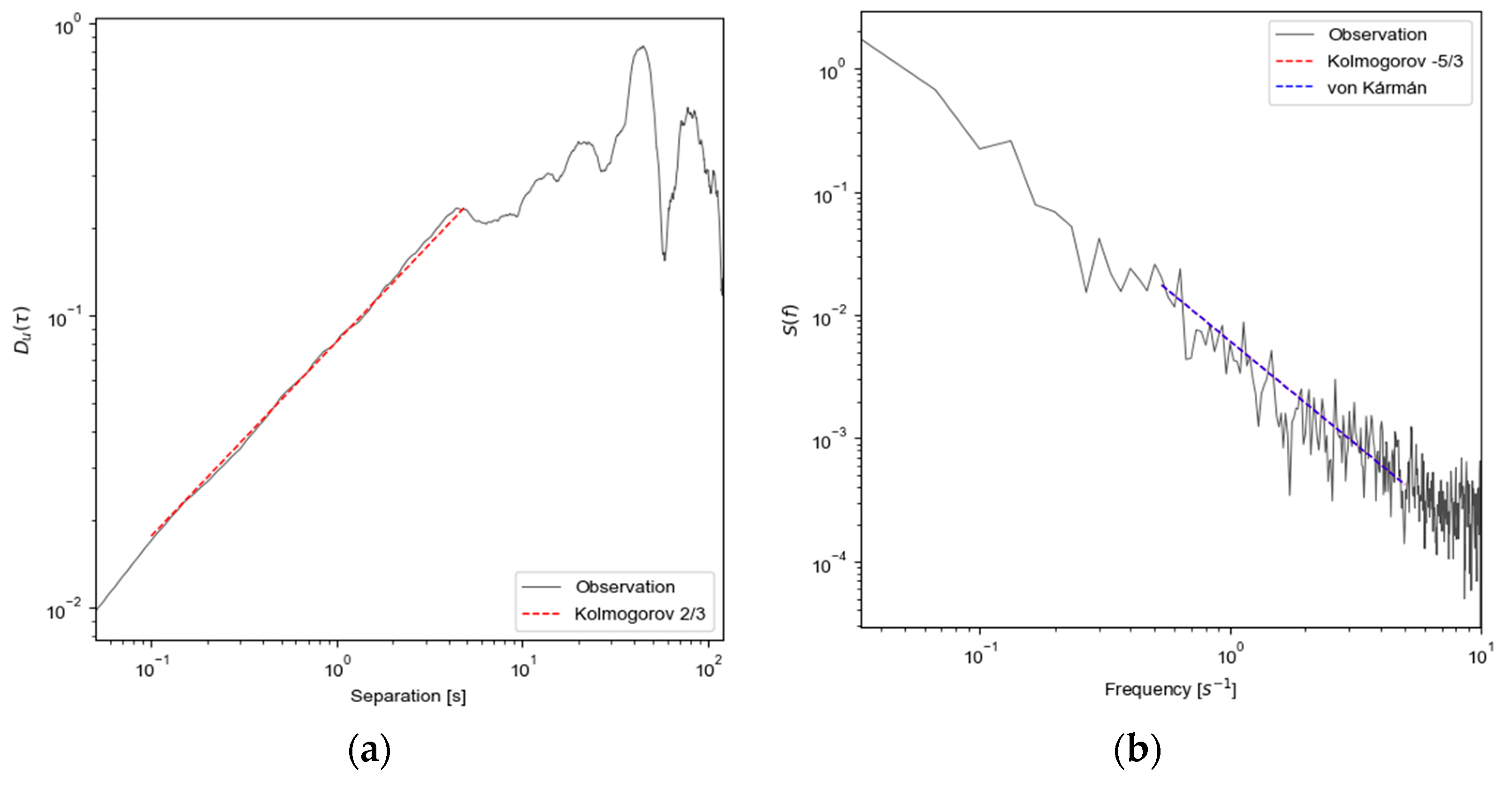
Figure 4a shows the observed SF and the theoretical SF from the Kolmogorov turbulence hypothesis at 60 m at 18:00 25 October 2018 local solar time (LST). The observed SF and the theoretical SF follow the 2/3 slope as expected by the Kolmogorov turbulence hypothesis within the predefined IR. In order to validate the use of IDM, the slopes of the observed SFs within the predefined IR were calculated for all levels and all seasons. The mean and median of the slopes were 0.542 and 0.555 with the percentage errors 18.7% and 16.7% relative to the theoretical value, 2/3.

3.2. Inertial Dissipation Method Using Spectral Density (EDR2) and Maximum Likelihood Estimation Using von Kármán Model (EDR3)

The relationship between EDR2 and PSD can be derived for frequencies within the IR assuming the Kolmogorov hypothesis [31,34]. After invoking Taylor’s frozen hypothesis:
EDR 2 = ( 2 π U ) 1 / 3 [ S u ( f ) f 5 / 3 ¯ C K 1 ] 1 / 2
where the overbar notation is the arithmetic average within IR. The PSD was obtained using a fast Fourier transform (FFT). Welch’s method was adopted [36,37], thus the 30-s subwindow with a 50% overlap was used. To reduce spurious signals due to discretization of the data, the Welch window function was applied to the subwindow.
Von Kármán suggested a spectral model for isotropic turbulence which includes a roll-off at the lower frequencies, as seen for example in Figure 4b. For the streamwise component, the PSD in the spatial domain is:
F model ( k ) = 9 55 α ε 2 / 3 1 ( L 2 + k 2 ) 5 / 6
where α is an empirical constant and L is the length scale [38]. α is set to 1.6 [9,38]. L is set to 500 feet as that is applicable for the level below 1000 ft [39], which is almost identical to the height of the tower. By substituting F ( k ) = U 2 π S ( f ) and k = U 2 π f , the von Kármán spectral model is expressed as a function of frequency. Maximum likelihood estimation between the observed spectra ( S o b s ) and the model spectra ( S m o d e l ) is applied to obtain the EDR through:
EDR 3 = [ 1 p 2 p 1 + 1 f = f 1 f 2 S obs ( f ) S model ( f ) ] 1 / 2
where f 1 and f 2 are the lower and upper bound frequencies of the IR, and p 1 and p 2 are the indices of f 1 and f 2 [9,40]. Here, the model spectra should correspond to an ε value of 1.0. The PSD and IR obtained in the retrieval of EDR2 were used to calculate EDR3.
First, we tested the IDM with the IR defined as the frequency range between 0.5 s−1 and 10 s−1, corresponding to the IR defined in the previous subsection [4]. Figure 4b shows the observed PSD and the expected PSDs from the Kolmogorov turbulence hypothesis and von Kármán spectral model at 60 m at 09:00 October 2018 LST. In general, the observed PSD follows well with the theoretical −5/3 slope as expected by both turbulence models within the predefined IR. However, at high frequencies, the observed PSD does not follow the expected −5/3 slope well. This might indicate that aliasing problems occur near the Nyquist frequency, and the 20 Hz sampling rate is not high enough to resolve turbulence structures with time scales shorter than 0.05 s. Here, the slopes of the PSDs within the predefined IR were calculated, and it was found that the mean and median were −1.163 and −1.189 with the percentage error of 30.2% and 28.6% compared to the theoretical value of −5/3. This discrepancy is probably due to aliasing problems. The PSD near the Nyquist frequency had a more positive slope than −5/3, and the PSD had more points as the frequency increased on the log-scale axis. As a result, the PSD near the Nyquist frequency was weighted higher in the estimation of the slope, which caused the slope to depart positively from the theoretical value. This might be a possible reason for the slightly higher EDR values in EDR2 and EDR3 than that in EDR1. Therefore, we defined the IR as the range between 0.5 s−1 and 5 s−1 to minimize aliasing effects which are shown as the theoretical Kolmogorov slope (red dashed line) and von Kármán spectral model (blue dashed line) in Figure 4b. After updating the IR for EDR2 and EDR3, we found that the mean and median of the slopes were now −1.374 and −1.423 with the percentage error reduced significantly to 17.5% and 14.6%. For this reason, the updated IR was adopted in the estimation of EDR2 and EDR3 in the rest of the paper.

4. Results and Discussion

4.1. Time Series of EDR and Its Variations

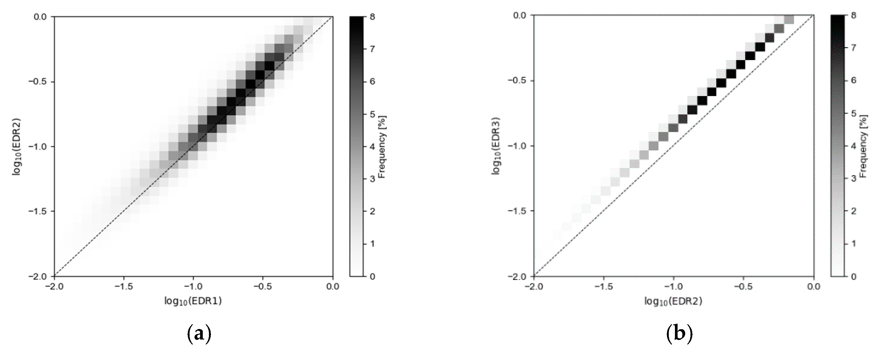
Time series of EDRs in the four seasons at the four levels were obtained using the above three different EDR estimation methods. Figure 5 shows the time series of 30-min block averaged EDRs in SON 2018. EDR2 and EDR3 were almost perfectly correlated for all levels because the Kolmogorov spectra and the von Kármán spectra are theoretically identical within the predefined IR in this study. On the other hand, the correlation coefficients between ln EDR 1 and ln EDR 2 ranged from 0.94 to 0.96, which is lower than that between EDR2 and EDR3. Nevertheless, it indicates that EDR1 and EDR2 are highly correlated and consistent although they originated from different estimation methods. To specify the relationships between the EDRs, 2D density scatter plots of the logarithms of EDRs were calculated and visualized as shown in Figure 6. EDR1 and EDR2 were reasonably consistent with the dispersion of the scatter plots. On the other hand, EDR2 and EDR3 showed almost perfect correspondence but with a systematic bias. These behaviors correspond to the correlation coefficients between EDRs and meet the finding in the previous section and other studies in which EDR was estimated using PSD was larger than that estimated using SF [4]. Although the PSD used in the estimation of EDR2 and EDR3 is identical and thus the results should be the same, EDR3 was found to be much larger than EDR2 and EDR1. This overestimation might be related to the maximum likelihood estimation used to estimate EDR3. There was no sensitivity in the slight change of the length scale because the IR was already defined far from the time scale affected by the change of the length scale (not shown).
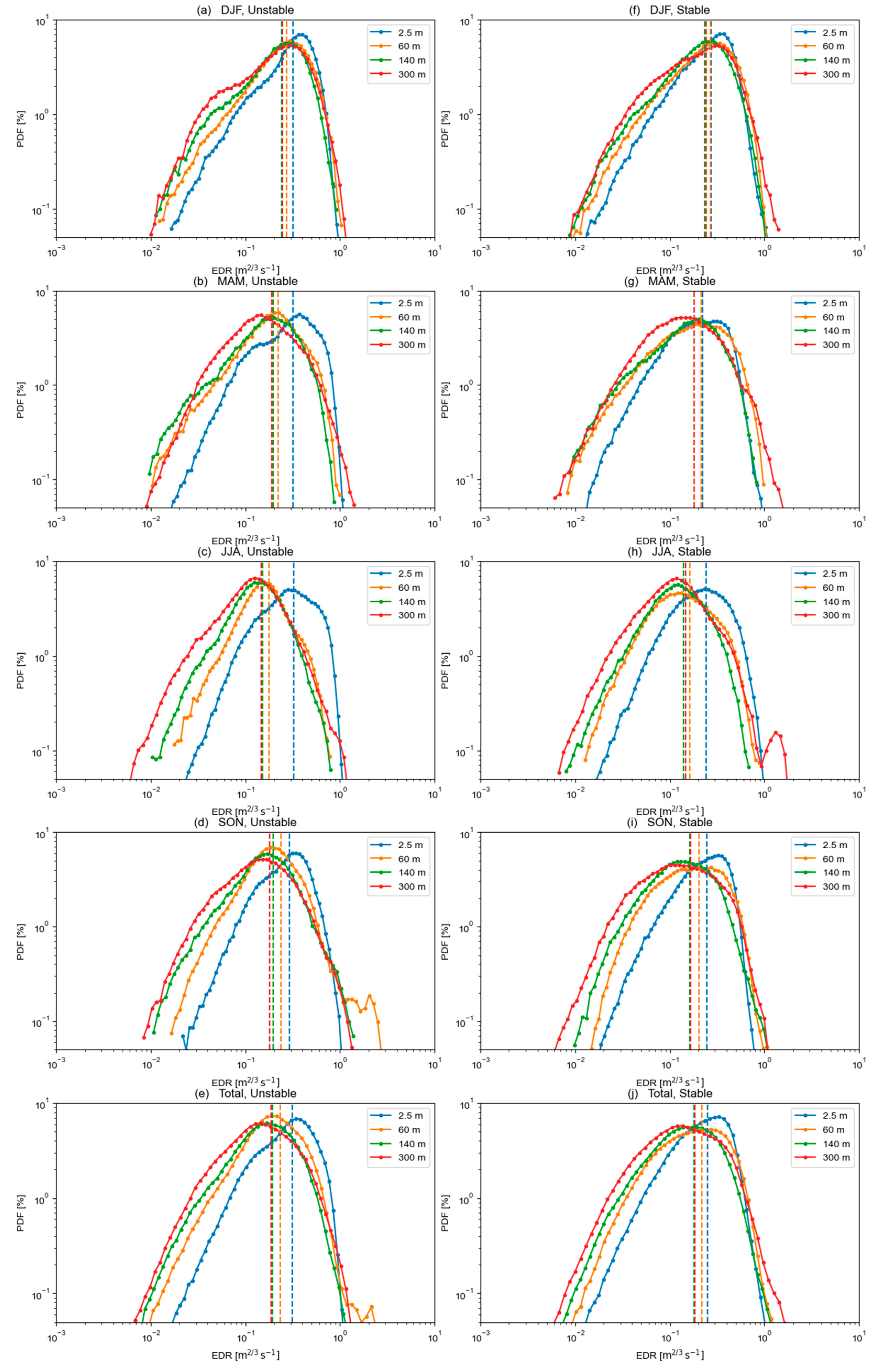
The diurnal variations in the EDRs were observed following the evolution of the PBL, especially between 20 September and 30 September 2018 (See Figure 5). In some periods, the diurnal variations were not evident perhaps due to external forcings such as low-pressure system passages, typhoons, and monsoon effects. For example, between 3 October to 15 October 2018 Korea was affected by a typhoon that passed directly over the BMO site on 5 October 2018, which swamped the diurnal variation effects. Overall, the diurnal variations were much more dominant in MAM and JJA compared to those in SON and DJF (not shown), i.e., the variations were stronger in the summertime than in the wintertime. One of the possible sources of such differences might be the incoming solar radiation and the background wind conditions. The incoming solar radiation drives the evolution of the PBL by increasing the buoyancy flux in the summertime. This increases TKE production in the daytime and ε compared to the nighttime. In contrast, the incoming solar radiation is less in the wintertime which decreases the difference of TKE production and ε between the daytime and the nighttime PBL, and the stronger background wind in the wintertime creates a larger shear production of TKE. As a result, in Table 2, the mean of ln EDR based on the EDR1 method (i.e., ln EDR ¯ ) at 2.5 m for the unstable PBL (daytime) in DJF is −1.3339, which is similar to that in JJA (−1.3352), but those for the stable PBL (nighttime) in DJF is −1.4817, which is much larger than that in JJA (−1.6236). Therefore, the difference between day and night in the wintertime is less than that in the summertime. The method to distinguish the unstable PBL (daytime) and the stable one (nighttime) and more detailed features in the PDFs of the observed EDRs will be discussed in the next section.

4.2. Characteristics of EDR and Application to Turbulence Forecasting

To investigate the characteristics of EDRs as a function of atmospheric stability, we classified the stability of the PBL using the sign of the Obukhov length, defined as:
L = u * 3 θ v ¯ κ g w θ v sfc
where κ is the von Kármán constant, g is gravity acceleration, u * is friction velocity, θ v is virtual potential temperature, and w θ v sfc is kinematic heat flux at 2.5 m above ground level. In the analysis, we approximated the virtual potential temperature θ v to the sonic temperature T s [41]. Here, κ = 0.4 and friction velocity, the kinematic heat flux, and the mean potential temperature with 30 min averaging were used to calculate the Obukhov length. The atmospheric stability is regarded as unstable if 500 < L 0 , stable if 0 < L < 500 , and neutral if L 500 or L > 500 [42]. Neutral atmospheric stability occurred about 5 to 9% out of the total and was neglected in this analysis. Only unstable and stable atmospheric stability were considered.
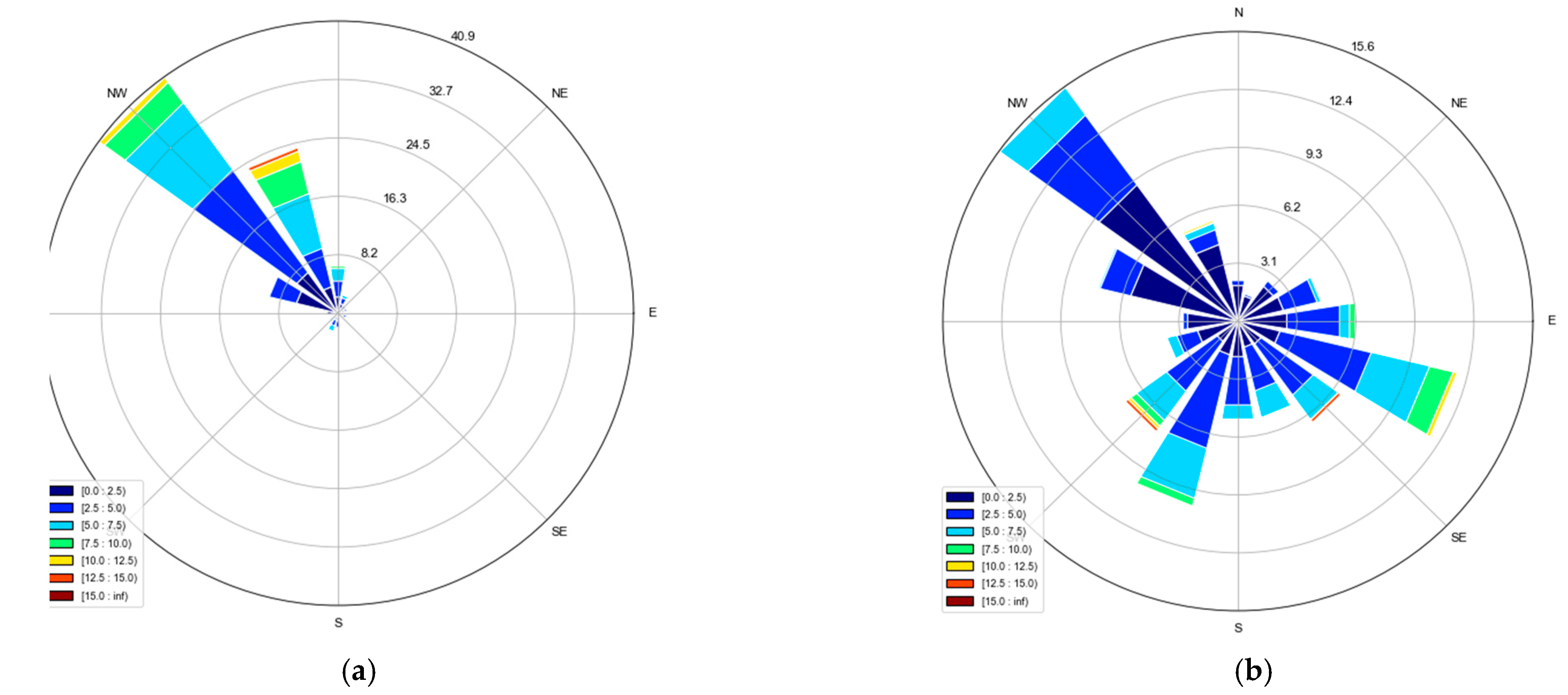
EDRs derived from the PSD-based models (EDR2 and EDR3) were similar to the EDR1 although it is likely to contain an aliasing problem as shown in the previous section so that the mean vertical structure and PDFs of EDR were calculated by using EDR1 only. Table 2 displays ln EDR ¯ and the standard deviations of ln EDR (i.e., SD ( ln EDR ) ) from January to December 2018 for each level and for each atmospheric stability. ln EDR ¯ decreased as height increased. In contrast, SD ( ln EDR ) increased as height increased. The interaction between the surface and turbulent flows were consistent regardless of the season and external forcings, implying that continuous forcings either by shear or buoyancy exist near the surface; therefore, the standard deviations were small. In a similar way, the variations of the mean in different seasons were typically the lowest at 2.5 m among all levels. Note that mean of ln EDR ranges from −1.339 (unstable DJF 2.5 m) to −2.2625 (stable JJA 300 m). In other words, EDR ranges from 0.1040 m2/3 s−1 (stable JJA 300 m) to 0.2634 m2/3 s−1 (unstable DJF 2.5 m). Qualitatively, the mean of ln EDR was smaller in the summertime than in the wintertime, due to the background wind condition with decreasing wind shear. Figure 7 presents the 30-min averaged wind direction with wind speed [43]. The westerly or northwesterly wind was dominant in the wintertime from the land mainly due to the East Asian winter monsoon (EAWM), with the continental high on the left and low-pressure system on the right, in the Korean peninsula provides a strong horizontal pressure gradient and gusty winds, implying larger shear production of TKE. In the summertime, however, the portion of southerly and southeasterly wind increased because of the weakened background wind with the more frequent activity of land-sea breeze at BMO [44], and thus contributed less TKE and turbulence dissipation. When we compare these EDR values with those from previous studies in different locations around the world, our EDR values are somewhat larger than that in most other areas, which is likely due to the strong background winds in winter and the location of BMO at the coastline where land-sea breezes are also dominant in summer.
Figure 8 shows the PDFs of EDR in the unstable and stable PBL. Given the situation that EAWM is dominant in winter and land-sea breezes are active in summer, it is obvious that the diurnal transition of the PDFs was not distinguished well, which is not surprising because the diurnal variations of EDR were not as strong as they were during the XPIA field campaign [4]. Since northwesterly winds were dominant regardless of the season, it is possible that this effect dominated over the diurnal evolution of EDR at BMO, and the shapes of PDFs became more uniform between day and night in the winter. The land-sea breeze in summer also disturbed the diurnal variations in the PDF of EDR at BMO. Qualitatively, the shape of the PDF followed the lognormal distribution in the stable PBL (nighttime). The shape of PDFs was also similar to the lognormal distribution even in the unstable PBL (daytime). Here, the log-Weibull-like distribution observed in [4] during unstable conditions was not observed. A notable feature in Figure 8 is that the PDFs at 2.5 m were separated from other levels because 2.5 m is near the surface where it is in the surface layer. As mentioned above, constant interaction between the surface and the atmosphere would force relatively strong turbulence dissipation and thus the shape of PDFs was skewed to the right near the surface.
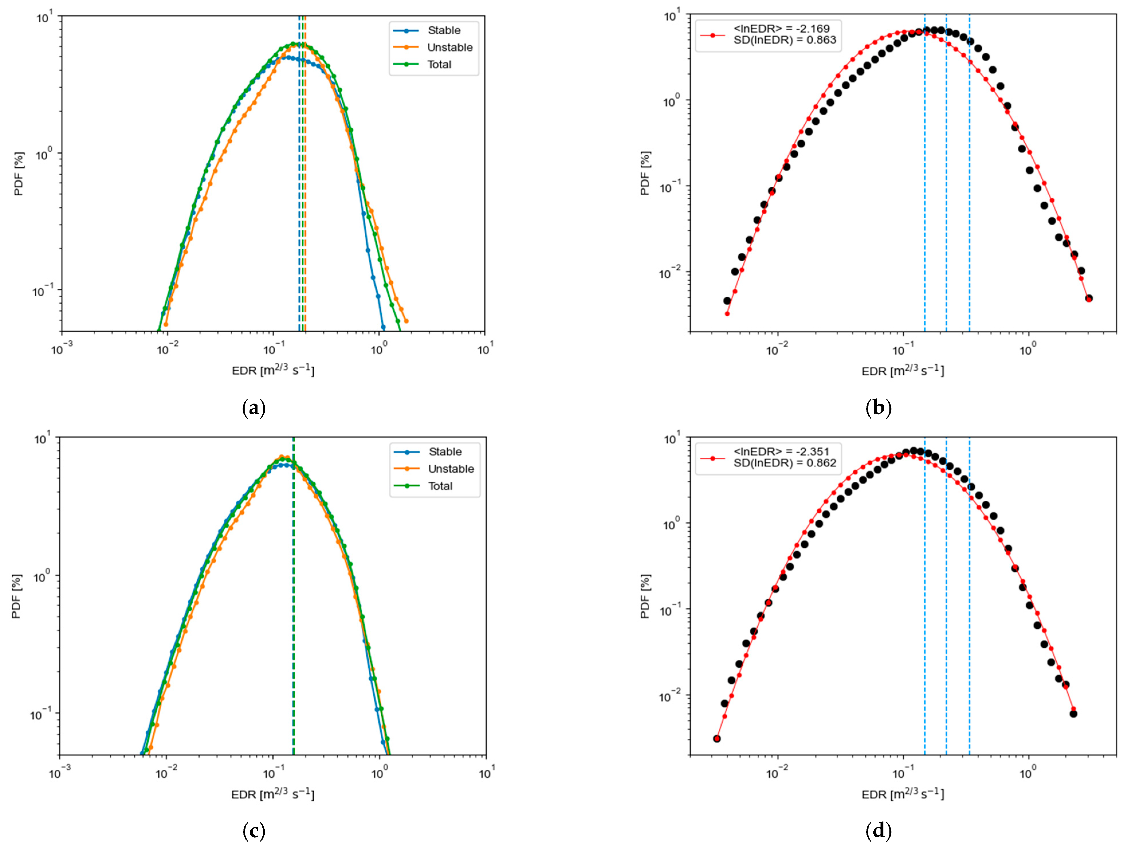
Finally, Figure 9 shows the PDFs of EDR for stable, unstable, and combined atmospheric stability at levels higher than 2.5 m (60 m ≤ z ≤ 300 m). In Figure 9a, the PDFs reasonably follow a lognormal distribution with similar shape parameters (i.e., μ and σ ) regardless of the atmospheric stability. This feature supports the observation that LLT at BMO has no significant change on the behavior of stable versus unstable PDFs, which is different from that in the XPIA result [4]. Therefore, we develop the best-fit curve using the single lognormal distribution for both the stable and unstable PBL. The PDFs for both stable and unstable cases were used to construct the best fit lognormal distribution curve as displayed in Figure 9b, showing that the lognormality was observed in the PDFs.
The climatological μ (mean of ln EDR ; ln EDR ) and σ (standard deviation of ln EDR ; SD ( ln EDR ) ) derived from the best-fit lognormal curve in Figure 9 are −2.169 and 0.863, respectively. These values are similar to the mean and standard deviations of ln EDR calculated directly from the observations as shown in Table 2. When we compare this result with those from commercial aircraft below 10,000 ft (about z = 3 km) in the U.S. [21], the mean value is similar but the standard deviation is larger at BMO. This is not surprising because the measurements in this study were closer to the surface than typical in-situ aircraft observations, implying that stronger fluctuations due to land-atmosphere interaction are expected.
To investigate the sensitivity of the results due to incorporation of the double rotation tilt correction, the PDF and its best-fit curve were produced after applying a double rotation algorithm [45], and are shown in Figure 9c,d. The skewness is reduced slightly, thus the shape follows a lognormal distribution compared to that with no tilt correction. The climatological mean and standard deviation are −2.351 and 0.862, respectively. Although double rotation is applied, the shapes of PDFs for each atmospheric stability are similar to each other, and the climatological mean and standard deviations do not change significantly, because BMO is located at a flat area near the coastline (Figure 1 and Figure 2).
Compared to previous studies, the mean and standard deviations of ln EDR derived from the shape parameters of the best-fit log-Weibull (lognormal) curve using the data from the XPIA field campaign were −2.1980 and 0.6564 (−2.7017 and 0.7641), respectively [6]. The median of the turbulence dissipation rate observed at the WFIP2 campaign roughly ranges from 5 × 10⁻⁴ m2 s−3 to 0.01 m2 s−3 [15], which corresponds to the range of −2.533 to −1.535 in terms of ln EDR . Considering that the WFIP2 campaign occurred in relatively heterogeneous terrain, it is expected that the mean value at BMO is closer to that observed in the WFIP2 campaign than that in the XPIA campaign. In addition to the surface heterogeneity, the stronger background wind is likely to force larger mean values at BMO than those in the previous studies.
Ultimately these statistics can be used to develop an LLT forecasting system based on the NWP model outputs with the LMT suitable for South Korea using the methodology of [6,21,22]. As described in the Introduction, LMT converts a turbulence diagnostic following a lognormal distribution to EDR using its mean and standard deviation. For a turbulence diagnostic D :
ln D * = a + b ln D
where D * is the EDR converted from D using LMT. a and b are remapping constants defined by the mean and standard deviations of each lognormal distribution of the turbulence diagnostic D and observed EDR ( ln EDR   SD ( ln EDR ) in Figure 9b,d) which are defined as:
a = ln EDR b ln D
b = S D ( ln EDR ) S D ( ln D )
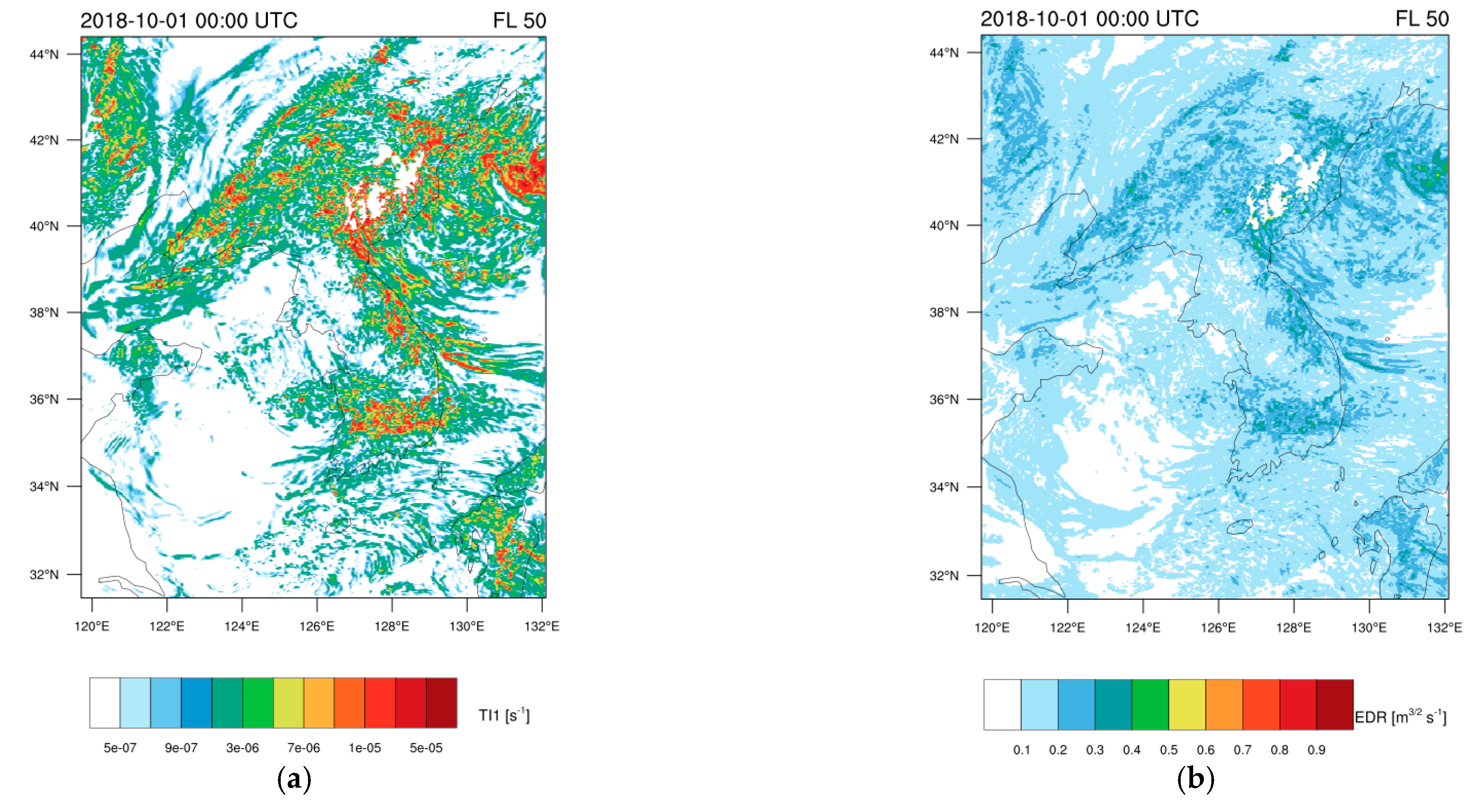
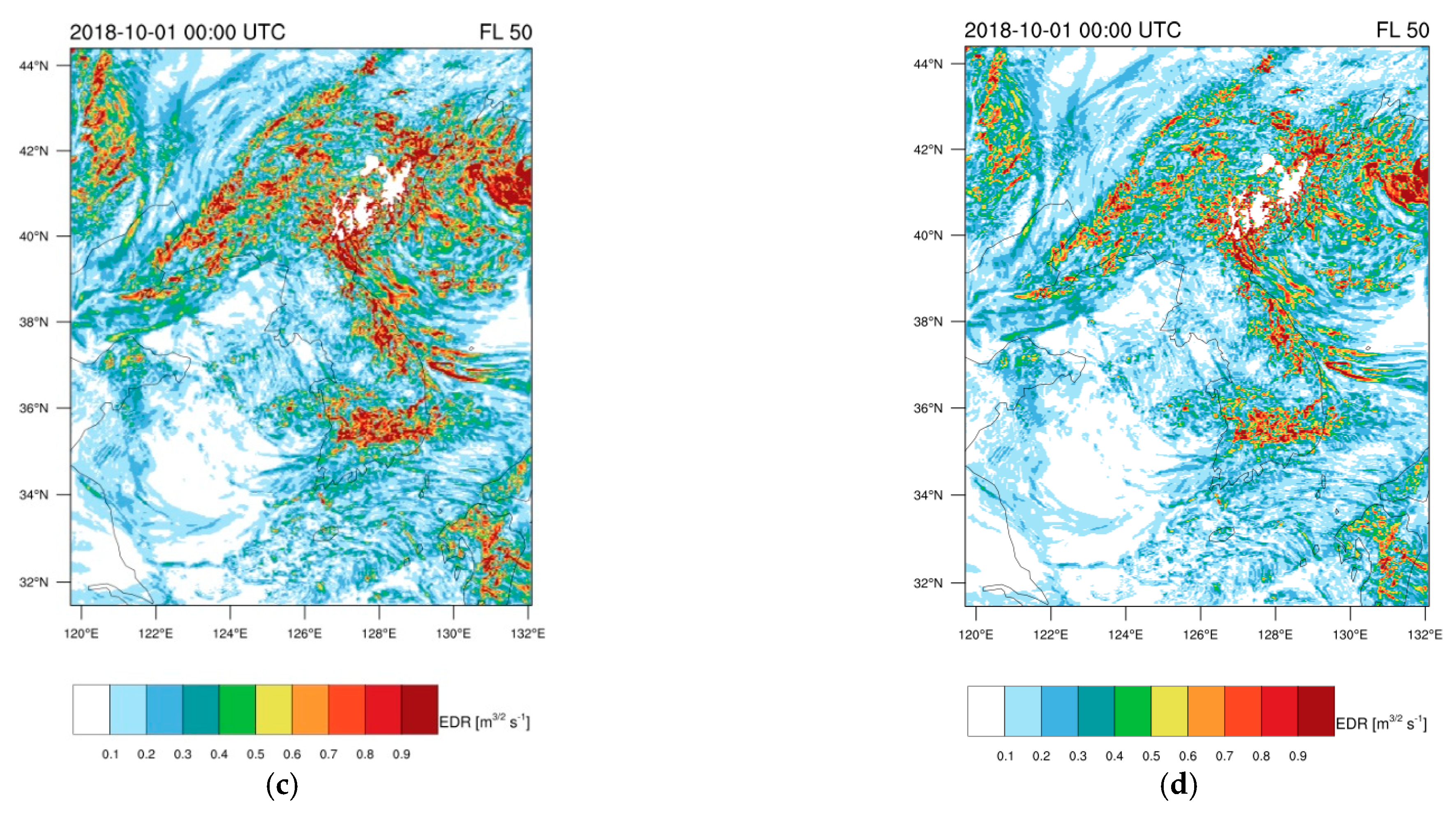
As an example, Figure 10 displays a horizontal distribution of the Ellrod TI1, an empirical turbulence diagnostic [46] and EDRs generated from LMT with climatological mean and standard deviations from [21] and BMO at FL050 (i.e., 5000 ft MSL in terms of barometric altitude) on 2018-10-01 00:00 UTC. Here, a mesoscale numerical simulation was conducted using the Weather Research and Forecasting Model [47], and the 3D components of simulated wind velocity were used to calculate the Ellrod TI1. Note that the mean and standard deviations of Ellrod TI1 were −15.3839 and 1.5895 for the regime below FL 100, respectively (not shown).
As exhibited in Figure 10c,d, the effect of double rotation algorithms is marginal but Figure 10c shows a slightly stronger derived turbulence intensity. Figure 10b significantly underestimates turbulence intensity compared to those in Figure 10c,d due to the smaller climatological standard deviations used. Figure 10c or Figure 10d can be used to forecast aviation turbulence with strong fluctuations at low levels, but the false alarm rate is likely to increase. On the other hand, Figure 10b is expected to show less false alarms, but it also may underpredict stronger events. To produce more skillful LLT forecasts, it will be necessary to have more statistics of the EDR derived from available observations such as lidar measurements, particularly near airports.

5. Conclusions

In this study, we investigated the characteristics of low-level turbulence (LLT) in South Korea as a function of the EDR observed at BMO with 20 Hz frequency sampling. There are two motivations for this study: (1) to develop an LLT forecast system based on the numerical weather prediction (NWP) models with the LMT method, which requires robust statistics (mean and standard deviation) of observed EDR for LLT; this will be beneficial for safe air-travel and air mobility in South Korea, and (2) to develop a better PBL parameterization within NWP models, it is necessary to understand the characteristics of LLT in heterogeneous areas like the BMO in coastal areas. With these goals in mind, we analyzed the time series and PDFs of the EDR from the wind data at four different levels (2.5 m, 60 m, 140 m, and 300 m above the ground) measured by the 20 Hz ultra-sonic anemometers. Three EDR estimation methods were tested based on different computational techniques (EDR1, EDR2, and EDR3). The key findings of this study are summarized as follows.
  • Although the EDR was estimated based on three different algorithms, the correlation coefficient of the time series of ln EDR s ranged from 0.94 to 0.96, which indicates that EDRs derived from each algorithm were highly correlated and consistent.
  • EDR1 was slightly lower than EDR2 regardless of the levels and seasons when we used the same IR, probably because of aliasing problems in EDR2. The difference of EDR1 and EDR2 reduced significantly when the shorter IR was used for EDR2. EDR3 was larger than EDR2 with a systematic bias. We conclude that EDR1, which avoids the aliasing problems is the most reliable estimation method, consistent with previous studies [4,6]. For a more thorough investigation of this, comparing the turbulence dissipation rate observed from hot-wire anemometers covering higher frequency ranges [3] is required.
  • A diurnal variation pattern was usually observed in the time series of the EDR. However, during some periods such variations were not dominant, likely related to the larger scale external forcings and background wind conditions such as synoptic low and high-pressure systems, typhoons, or monsoons.
  • For each season, ln EDR ¯ decreased with height whereas, SD ( ln EDR ) increased with height. This behavior likely arises from the continuous interactions between the surface and turbulent flows. ln EDR ¯ was typically larger in the wintertime than in the summertime and is related to the intensity of background wind (i.e., wind shear).
  • There was no strong diurnal transition of the PDFs of EDR between the lognormal distribution and log-Weibull distribution regardless of the atmospheric stability and season, which can be explained by the background wind flows in wintertime and dominant land-sea breeze events in the summertime.
  • LMT was conducted using only a single lognormal distribution curve for the observed PDF of EDR. The statistics (mean and standard deviations of ln EDR ) required to develop an LLT forecasting system using the methodology of [6,19,21,22] were obtained. For the levels above 2.5 m in SON, ln EDR and SD ( ln EDR ) were −2.169 and 0.863, respectively. With the above statistics, an example of low-level turbulence forecasting was presented using the Ellrod TI1 turbulence diagnostic.
To further examine the climatology and the representativeness of these results, the present analysis will be expanded to include longer time periods using the multi-year measurements from BMO in a future study. At the same time, the mesoscale numerical simulations focusing on the low-level environment around BMO will be conducted using high-resolution NWP models with various PBL schemes. In 1.5-order closure PBL schemes, turbulence dissipation rate is parameterized using TKE, and EDR is expressed as a function of TKE and a master length scale. Large-eddy simulations (LES) that can fully resolve daytime large eddies will also be used to estimate the TKE and EDRs in various seasons in Korea and to retrieve turbulence quantities such as shear or buoyancy production. Land-sea breezes at Boseong might affect the local circulations and the vertical structure of the PBL and thus the EDR. The effects of the land-sea breeze on the vertical structure of the PBL can be investigated by mesoscale NWP modeling [48,49]. Based on either 1.5-order closure TKE PBL schemes or LES modeling with subfilter-scale parameterizations, the range of values and correlations will be compared using the observed EDRs and simulated EDRs. Moreover, we will interpret the physical mechanisms of the various properties of PDFs exhibited in this study using the simulated environmental conditions with the focus on the effect of land-sea breeze circulations at Boseong.

Author Contributions

Conceptualization, J.K.; Formal analysis, J.K., J.-H.K. and R.D.S.; Funding acquisition, J.-H.K.; Investigation, J.K., J.-H.K. and R.D.S.; Methodology, J.-H.K. and R.D.S.; Project administration, J.-H.K.; Resources, J.-H.K.; Software, J.K.; Supervision, J.-H.K.; Validation, J.K., J.-H.K. and R.D.S.; Visualization, J.K.; Writing—original draft, J.K. and J.-H.K.; Writing—review & editing, J.-H.K. and R.D.S. All authors have read and agreed to the published version of the manuscript.

Funding

This research was supported by the Basic Science Research Program through the National Research Foundation of Korea (NRF) funded by the Ministry of Education (NRF- 2019R1I1A2A1060035).

Data Availability Statement

EDR data presented in this study are available on request from the corresponding author.

Acknowledgments

This work was supported by the Basic Science Research Program through the National Research Foundation of Korea (NRF) funded by the Ministry of Education (NRF- 2019R1I1A2A1060035). We thank the researchers at the National Institute of Meteorological Sciences for access to observation data in Boseong.

Conflicts of Interest

The authors declare no conflict of interest.

References

  1. Cornman, L.; Morse, C.; Cunning, G. Real-time estimation of atmospheric turbulence severity from In Situ aircraft measure-ments. J. Aircr. 1995, 32, 171–177. [Google Scholar] [CrossRef]
  2. ICAO. Meteorological Service for International Air Navigation, 17th ed.; ICAO: Montreal, CA, Canada, 2010; p. 206. [Google Scholar]
  3. Piper, M.; Lundquist, J.K. Surface Layer Turbulence Measurements during a Frontal Passage. J. Atmos. Sci. 2004, 61, 1768–1780. [Google Scholar] [CrossRef]
  4. Muñoz-Esparza, D.; Sharman, R.D.; Lundquist, J.K. Turbulence dissipation rate in the atmospheric boundary layer: Observa-tions and WRF mesoscale modeling during the XPIA field campaign. Mon. Weather Rev. 2018, 146, 351–371. [Google Scholar] [CrossRef] [Green Version]
  5. Lundquist, J.K.; Bariteau, L. Dissipation of Turbulence in the Wake of a Wind Turbine. Bound. Layer Meteorol. 2014, 154, 229–241. [Google Scholar] [CrossRef]
  6. Muñoz-Esparza, D.; Sharman, R. An Improved Algorithm for Low-Level Turbulence Forecasting. J. Appl. Meteorol. Clim. 2018, 57, 1249–1263. [Google Scholar] [CrossRef]
  7. Bodini, N.; Lundquist, J.K.; Newsom, R.K. Estimation of turbulence dissipation rate and its variability from sonic anemometer and wind Doppler lidar during the XPIA field campaign. Atmos. Meas. Tech. 2018, 11, 4291–4308. [Google Scholar] [CrossRef] [Green Version]
  8. Večenaj, Ž.; Belušić, D.; Grisogono, B. Characteristics of the near-surface turbulence during a bora event. Ann. Geophys. 2010, 28, 155–163. [Google Scholar] [CrossRef] [Green Version]
  9. Sharman, R.D.; Cornman, L.B.; Meymaris, G.; Pearson, J.; Farrar, T. Description and Derived Climatologies of Automated In Situ Eddy-Dissipation-Rate Reports of Atmospheric Turbulence. J. Appl. Meteorol. Clim. 2014, 53, 1416–1432. [Google Scholar] [CrossRef]
  10. Strauss, L.; Serafin, S.; Haimov, S.; Grubišić, V. Turbulence in breaking mountain waves and atmospheric rotors estimated from airborne in situ and Doppler radar measurements. Q. J. R. Meteorol. Soc. 2015, 141, 3207–3225. [Google Scholar] [CrossRef] [PubMed]
  11. Bramberger, M.; Dörnbrack, A.; Wilms, H.; Ewald, F.; Sharman, R. Mountain-Wave Turbulence Encounter of the Research Aircraft HALO above Iceland. J. Appl. Meteorol. Clim. 2020, 59, 567–588. [Google Scholar] [CrossRef]
  12. Frehlich, R.; Meillier, Y.; Jensen, M.L. Measurements of Boundary Layer Profiles with In Situ Sensors and Doppler Lidar. J. Atmos. Ocean. Technol. 2008, 25, 1328–1340. [Google Scholar] [CrossRef]
  13. Chan, P.W. Generation of an Eddy Dissipation Rate Map at the Hong Kong International Airport Based on Doppler Lidar Data. J. Atmos. Ocean. Technol. 2011, 28, 37–49. [Google Scholar] [CrossRef]
  14. Hon, K.K.; Chan, P.W. Application of LIDAR-derived eddy dissipation rate profiles in low-level wind shear and turbulence alerts at Hong Kong International Airport. Meteorol. Appl. 2014, 21, 74–85. [Google Scholar] [CrossRef]
  15. Bodini, N.; Lundquist, J.K.; Krishnamurthy, R.; Pekour, M.; Berg, L.K.; Choukulkar, A. Spatial and temporal variability of turbulence dissipation rate in complex terrain. Atmos. Chem. Phys. 2019, 19, 4367–4382. [Google Scholar] [CrossRef] [Green Version]
  16. Bodini, N.; Lundquist, J.K.; Kirincich, A.U.S. East Coast Lidar Measurements Show Offshore Wind Turbines Will Encounter Very Low Atmospheric Turbulence. Geophys. Res. Lett. 2019, 46, 5582–5591. [Google Scholar] [CrossRef] [Green Version]
  17. Wildmann, N.; Bodini, N.; Lundquist, J.K.; Bariteau, L.; Wagner, J. Estimation of turbulence dissipation rate from Doppler wind lidars and in situ instrumentation for the Perdigão 2017 campaign. Atmos. Meas. Tech. 2019, 12, 6401–6423. [Google Scholar] [CrossRef] [Green Version]
  18. Nijhuis, A.C.P.O.; Unal, C.M.H.; Krasnov, O.A.; Russchenberg, H.W.J.; Yarovoy, A.G. Velocity-Based EDR Retrieval Tech-niques Applied to Doppler Radar Measurements from Rain: Two Case Studies. J. Atmos. Ocean. Technol. 2019, 36, 1693–1711. [Google Scholar] [CrossRef] [Green Version]
  19. Kim, J.-H.; Park, J.-R.; Kim, S.-H.; Kim, J.; Lee, E.; Baek, S.; Lee, G. A Detection of Convectively Induced Turbulence Using in Situ Aircraft and Radar Spectral Width Data. Remote. Sens. 2021, 13, 726. [Google Scholar] [CrossRef]
  20. Nastrom, G.D.; Gage, K.S. A Climatology of Atmospheric Wavenumber Spectra of Wind and Temperature Observed by Commercial Aircraft. J. Atmos. Sci. 1985, 42, 950–960. [Google Scholar] [CrossRef] [Green Version]
  21. Sharman, R.D.; Pearson, J.M. Prediction of Energy Dissipation Rates for Aviation Turbulence. Part I: Forecasting Nonconvective Turbulence. J. Appl. Meteorol. Clim. 2017, 56, 317–337. [Google Scholar] [CrossRef]
  22. Kim, J.-H.; Sharman, R.; Strahan, M.; Scheck, J.W.; Bartholomew, C.; Cheung, J.C.H.; Buchanan, P.; Gait, N. Improvements in Nonconvective Aviation Turbulence Prediction for the World Area Forecast System. Bull. Am. Meteorol. Soc. 2018, 99, 2295–2311. [Google Scholar] [CrossRef] [Green Version]
  23. Lundquist, J.K.; Wilczak, J.M.; Ashton, R.; Bianco, L.; Brewer, W.A.; Choukulkar, A.; Clifton, A.; Debnath, M.; Delgado, R.; Friedrich, K.; et al. Assessing State-of-the-Art Capabilities for Probing the Atmospheric Boundary Layer: The XPIA Field Campaign. Bull. Am. Meteorol. Soc. 2017, 98, 289–314. [Google Scholar] [CrossRef]
  24. Wilczak, J.M.; Stoelinga, M.; Berg, L.K.; Sharp, J.; Draxl, C.; McCaffrey, K.; Banta, R.M.; Bianco, L.; Djalalova, I.; Lundquist, J.K.; et al. The Second Wind Forecast Improvement Project (WFIP2): Observational Field Campaign. Bull. Am. Meteorol. Soc. 2019, 100, 1701–1723. [Google Scholar] [CrossRef]
  25. Wilczak, J.M.; Oncley, S.P.; Stage, S.A. Sonic Anemometer Tilt Correction Algorithms. Bound. Layer Meteorol. 2001, 99, 127–150. [Google Scholar] [CrossRef]
  26. Frank, J.M.; Massman, W.J.; Ewers, B.E. Underestimates of sensible heat flux due to vertical velocity measurement errors in non-orthogonal sonic anemometers. Agric. For. Meteorol. 2013, 171–172, 72–81. [Google Scholar] [CrossRef]
  27. Grelle, A.; Lindroth, A. Flow Distortion by a Solent Sonic Anemometer: Wind Tunnel Calibration and Its Assessment for Flux Measurements over Forest and Field. J. Atmos. Ocean. Technol. 1994, 11, 1529–1542. [Google Scholar] [CrossRef] [Green Version]
  28. Loescher, H.; Ocheltree, T.; Tanner, B.; Swiatek, E.; Dano, B.; Wong, J.; Zimmerman, G.; Campbell, J.; Stock, C.; Jacobsen, L.; et al. Comparison of temperature and wind statistics in contrasting environments among different sonic anemometer–thermometers. Agric. For. Meteorol. 2005, 133, 119–139. [Google Scholar] [CrossRef]
  29. Dyer, A.J. Flow distortion by supporting structures. Bound. Layer Meteorol. 1981, 20, 243–251. [Google Scholar] [CrossRef]
  30. Taylor, G.I.; Null, N. Statistical theory of turbulence. Proc. R. Soc. A Math. Phys. Eng. Sci. 1935, 151, 421–444. [Google Scholar] [CrossRef] [Green Version]
  31. Pope, S. Turbulent Flows; Cambridge University Press: Cambridge, UK, 2000; 771p. [Google Scholar]
  32. Higgins, C.W.; Froidevaux, M.; Simeonov, V.; Vercauteren, N.; Barry, C.; Parlange, M. The Effect of Scale on the Applicability of Taylor’s Frozen Turbulence Hypothesis in the Atmospheric Boundary Layer. Bound. Layer Meteorol. 2012, 143, 379–391. [Google Scholar] [CrossRef] [Green Version]
  33. Kolmogorov, A.N. The local structure of turbulence in incompressible viscous fluid for very large Reynolds numbers. Akad. Nauk SSSR Dokl. 1941, 30, 301–305. [Google Scholar]
  34. Tennekes, H.; Lumley, J.L. A First Course in Turbulence; MIT Press: Cambridge, MA, USA, 1972; 320p. [Google Scholar]
  35. Champagne, F.H.; Friehe, C.A.; LaRue, J.C.; Wynagaard, J.C. Flux Measurements, Flux Estimation Techniques, and Fine-Scale Turbulence Measurements in the Unstable Surface Layer Over Land. J. Atmos. Sci. 1977, 34, 515–530. [Google Scholar] [CrossRef] [Green Version]
  36. Welch, P. The use of fast Fourier transform for the estimation of power spectra: A method based on time averaging over short, modified periodograms. IEEE Trans. Audio Electroacoust. 1967, 15, 70–73. [Google Scholar] [CrossRef] [Green Version]
  37. Virtanen, P.; Gommers, R.; Oliphant, T.E.; Haberland, M.; Reddy, T.; Cournapeau, D.; Burovski, E.; Peterson, P.; Weckesser, W.; Bright, J.; et al. SciPy 1.0: Fundamental algorithms for scientific computing in Python. Nat. Methods 2020, 17, 261–272. [Google Scholar] [CrossRef] [PubMed] [Green Version]
  38. Mann, J. The spatial structure of neutral atmospheric surface-layer turbulence. J. Fluid Mech. 1994, 273, 141–168. [Google Scholar] [CrossRef]
  39. Austin, W.H. The Effects of Low Level Turbulence on the Structure of a Large Logistic Aircraft. SAE Tech. Pap. Ser. 1966. [Google Scholar] [CrossRef]
  40. Cornman, L.B. Airborne In Situ Measurements of Turbulence. In Aviation Turbulence: Processes, Detection, Prediction, 1st ed.; Sharman, R., Lane, T., Eds.; Springer International Publishing: Cham, Switzerland, 2016; pp. 97–120. [Google Scholar]
  41. Bodini, N.; Lundquist, J.K.; Optis, M. Can machine learning improve the model representation of turbulent kinetic energy dissipation rate in the boundary layer for complex terrain? Geosci. Model Dev. 2020, 13, 4271–4285. [Google Scholar] [CrossRef]
  42. Muñoz-Esparza, D.; Cañadillas, B.; Neumann, T.; van Beeck, J. Turbulent fluxes, stability and shear in the offshore environ-ment: Mesoscale modelling and field observations at FINOJ. Renew. Sustain. Energy 2012, 4, 63136. [Google Scholar] [CrossRef]
  43. Roubeyrie, L.; Celles, S. Windrose: A Python Matplotlib, Numpy library to manage wind and pollution data, draw windrose. J. Open Source Softw. 2018, 3, 268. [Google Scholar] [CrossRef]
  44. Lim, H.-J.; Lee, Y.-H. Characteristics of Sea Breezes at Coastal Area in Boseong. Atmosphere 2019, 29, 41–51. (In Korean) [Google Scholar]
  45. Cheynet, E. Tilt-Correction Algorithms for 3D Sonic Anemometers. 2020. Available online: https://zenodo.org/record/3922252#.YNqSJUwRWUl (accessed on 31 March 2021).
  46. Ellrod, G.P.; Knapp, D.I. An Objective Clear-Air Turbulence Forecasting Technique: Verification and Operational Use. Weather. Forecast. 1992, 7, 150–165. [Google Scholar] [CrossRef] [Green Version]
  47. Skamarock, W.C.; Klemp, J.B.; Dudhia, J.; Gill, D.O.; Liu, Z.; Berner, J.; Wang, W.; Powers, J.G.; Duda, M.G.; Barker, D.; et al. A Description of the Advanced Research WRF Model Version 4; Technical Report; UCAR/NCAR: Boulder, CO, USA, 2019. [Google Scholar]
  48. Ryu, Y.-H.; Baik, J.-J. Daytime Local Circulations and Their Interactions in the Seoul Metropolitan Area. J. Appl. Meteorol. Clim. 2013, 52, 784–801. [Google Scholar] [CrossRef]
  49. Ganbat, G.; Baik, J.-J.; Ryu, Y.-H. A numerical study of the interactions of urban breeze circulation with mountain slope winds. Theor. Appl. Clim. 2015, 120, 123–135. [Google Scholar] [CrossRef]
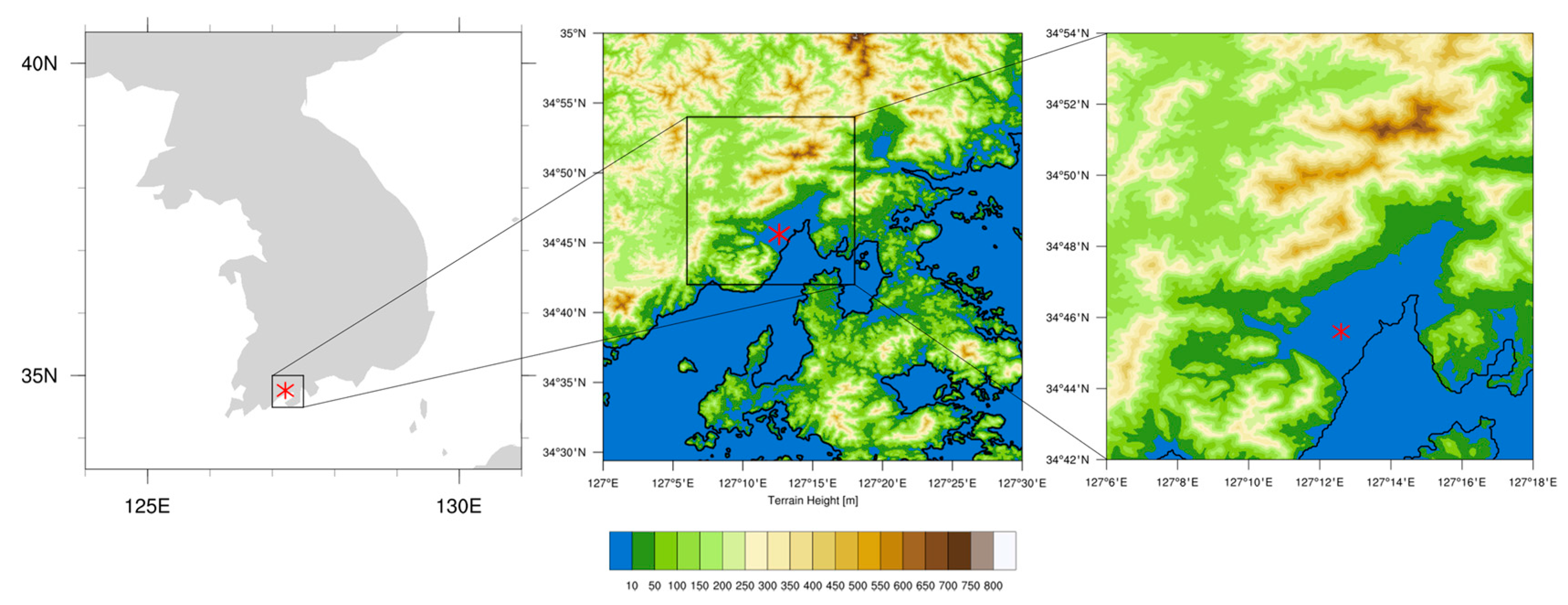
Figure 1. Map of the Korean Peninsula and the local maps around BMO with terrain height (shadings) and local coastlines (solid black line). The location of BMO (34.76° N and 127.21° E) is marked by red asterisks.
Atmosphere 12 00837 g001
Figure 2. (Left) Bird’s eye view of BMO (In this photo, north is on the left and south is on the right), and (Right) the 307 m meteorological tower established at BMO. Four 3D sonic anemometers are mounted at 60 m, 140 m, and 300 m above the ground, on the northeastern side of the observation boom. Additionally, a 3D sonic anemometer is installed at 2.5 m above the ground located to the southeast of the tower (white box at the top of the left photo). An automated surface observing system (ASOS) is also located in BMO (white box at the bottom of the left photo).
Atmosphere 12 00837 g002
Figure 3. The available and the missing portion of produced EDR at the four levels. Green color indicates that EDR was produced and regarded as reliable, while red color indicates that EDR was not produced and regarded as missing at the given time.
Atmosphere 12 00837 g003
Figure 4. SFs and PSDs of EDR at 60 m at 18:00 25 October 2018 LST. The length of the red and blue lines indicate the IR range used in the calculation. (a) (black) the observed SF from the anemometer and (red) the theoretical SF expected for Table 1. (0.2169 m2/3 s−1) by Kolmogorov turbulence hypothesis; (b) (black) the observed PSD from the anemometer, (red) the theoretical PSD expected for the estimated EDR2 (0.2113 m2/3 s−1) by the Kolmogorov turbulence hypothesis, and (blue) the theoretical PSD for the estimated EDR3 (0.2978 m2/3 s−1) by the von Kármán spectral model. Note that the red and blue lines in (b) are closely overlapped.
Atmosphere 12 00837 g004
Figure 5. Time series of 30-min block averaged (red) EDR1, (orange) EDR2, and (green) EDR3 at (a) 300 m, (b) 140 m, (c) 60 m, and (d) 2.5 m in SON. Empty space indicates that EDRs were not produced and set to missing at the given time.
Atmosphere 12 00837 g005
Figure 6. 2D density scatter plots between (a) log 10 EDR 1 and log 10 EDR 2 , and (b) log 10 EDR 2 and log 10 EDR 3 , calculated from the EDRs at the four levels in 2018. Bins with darker color indicate that more elements were counted within these bins.
Atmosphere 12 00837 g006
Figure 7. Windroses generated from 30-min averaged wind direction and wind speed observed at the sonic anemometer at 60 m (a) in the wintertime (DJF), and (b) in the summertime (JJA) [43]. The label bar indicates the wind speed for the given wind direction bin. The radius indicates the percentage of the portion out of total for the given bin.
Atmosphere 12 00837 g007
Figure 8. PDFs of EDR. Left panel shows the PDFs for the unstable PBL in (a) DJF, (b) MAM, (c) JJA, (d) SON, and (e) total in 2018, and for the stable PBL in (f) DJF, (g) MAM, (h) JJA, and (i) SON, and (j) total in 2018, at 2.5 m (blue solid line), 60 m (orange solid line), 140 m (green solid line), and 300 m (red solid line). Dashed line indicates mean of EDR1 in the given season at the given level.
Atmosphere 12 00837 g008
Figure 9. (a) PDFs of the EDR for (blue) stable and (orange) unstable planetary boundary layers (PBL), (green) PDF of the EDR regardless of the atmospheric stability, and (b) (red line) the best-fit lognormal curve for (black dots) the observed PDF of the EDR where the black dots correspond to the green line in (a). (c) Same as (a) but double rotation was applied, and (d) same as (b) but double rotation was applied. Atmospheric stability in (a) was classified by using the Obukhov length defined in Equation (11). Blue vertical lines in (b) show the thresholds of EDR values, 0.15 m2/3 s−1, 0.22 m2/3 s−1, and 0.33 m2/3 s−1, which correspond to the light (LGT), moderate (MOD), and severe (SEV) turbulence intensities for mid-size aircraft like B-737.
Atmosphere 12 00837 g009
Figure 10. Horizontal distributions at FL050 (approximately 5000 ft) generated from (a) Ellrod TI1 and (b) EDR converted from Ellrod TI1 using LMT and the climatological mean and standard deviations presented in [21] ( ln EDR = 2.248 and SD ( ln EDR ) = 0.4235 for the altitude region below FL100). (c) Same as (b) but climatological values at Figure 9b ( ln EDR = 2.169 and SD ( ln EDR ) = 0.863 ) were used. (d) Same as (b) but climatological values at Figure 9d ( ln EDR = 2.351 and SD ( ln EDR ) = 0.862 ) were used.
Atmosphere 12 00837 g010aAtmosphere 12 00837 g010b
Table 1. The portion of the missing values of EDR in the winter, spring, summer, fall, and for the total one-year period. The unit is %.
DJFMAMJJASONTotal
2.5 m4.57313.0110.678.4039.194
60 m2.52153.6537.6610.2426.19
140 m16.6754.3621.5916.2227.30
300 m16.9010.9812.609.98212.60
Table 2. The mean and the standard deviations of ln EDR 1 in the (top) unstable and (bottom) stable PBL, for each season (DJF, MAM, JJA, and SON), and for the 1-yr period (Total) in 2018.
Mean   of   ln E D R ( Unstable )
DJFMAMJJASONTotal
2.5 m−1.3339−1.3707−1.3352−1.4085−1.3609
60 m−1.5241−1.7690−1.9088−1.7082−1.7122
140 m−1.6713−1.9174−2.0961−1.9120−1.9138
300 m−1.7167−1.9680−2.2182−2.0526−2.0108
Standard Deviation of ln EDR (Unstable)
DJFMAMJJASONTotal
2.5 m0.69520.75260.67900.64160.6964
60 m0.76510.80700.64070.72480.7479
140 m0.80210.84490.69460.79540.7913
300 m0.87550.83810.80700.85540.8583
Mean of ln EDR (Stable)
DJFMAMJJASONTotal
2.5 m−1.4817−1.7373−1.6236−1.5721−1.5942
60 m−1.5769−1.8765−2.0644−1.8515−1.8087
140 m−1.7164−2.0239−2.1934−2.0883−1.9979
300 m−1.7396−2.0732−2.2625−2.1722−2.0648
Standard Deviation of ln EDR (Stable)
DJFMAMJJASONTotal
2.5 m0.69530.73560.68960.64530.6951
60 m0.79460.89600.76690.78510.8206
140 m0.80170.88460.74160.77850.8142
300 m0.88590.90150.83100.90590.9047
Publisher’s Note: MDPI stays neutral with regard to jurisdictional claims in published maps and institutional affiliations.