
ECLand: The ECMWF Land Surface Modelling System


 ,
, 
 , ,
, ,  , ,
, ,
Abstract
1. Introduction
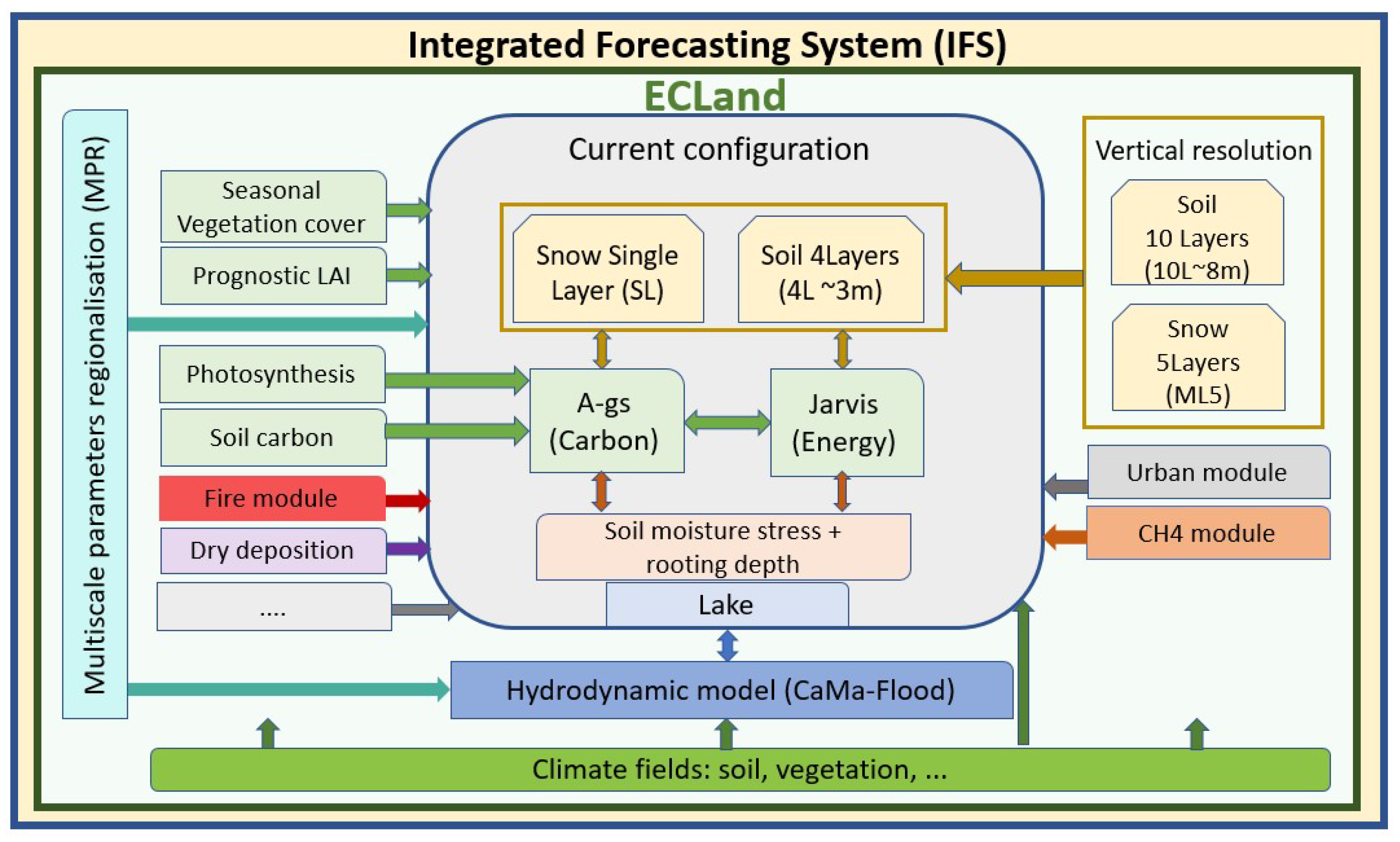
2. Model Description
3. Model Development
3.1. Land Biosphere Representation
3.1.1. Land Use/Land Cover and Leaf Area Index
3.1.2. Dynamic Vegetation
Seasonal Vegetation Cover
Prognostic Vegetation Parameterisation
3.2. Updated Snow Parametrization
3.3. Updated Soil Parametrization
3.4. Surface Water Representation
3.5. Coupling with a Hydrodynamic Model
3.6. Urban Parametrization
3.7. Model Efficiency
4. Evaluation of Model Developments
4.1. Data and Methods
4.2. Observational Data to Evaluate Model Developments
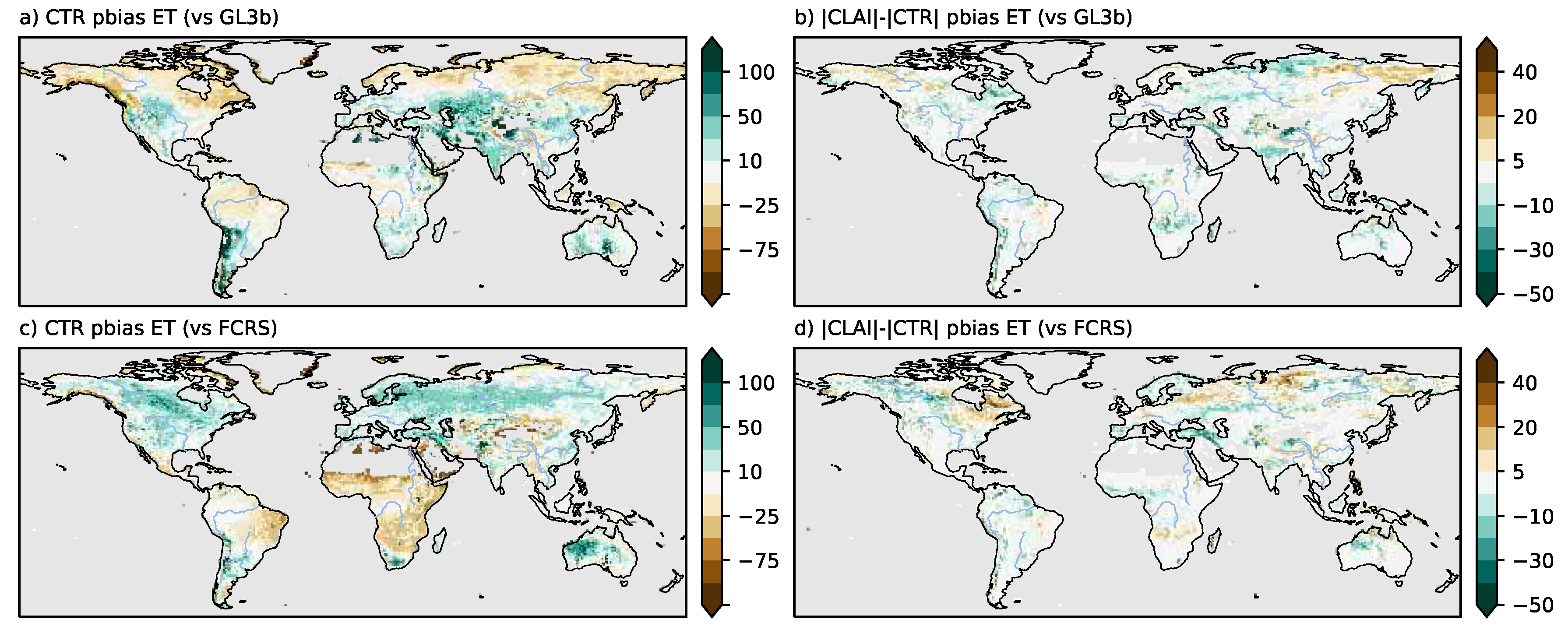
4.2.1. FluxCom
4.2.2. GLEAM
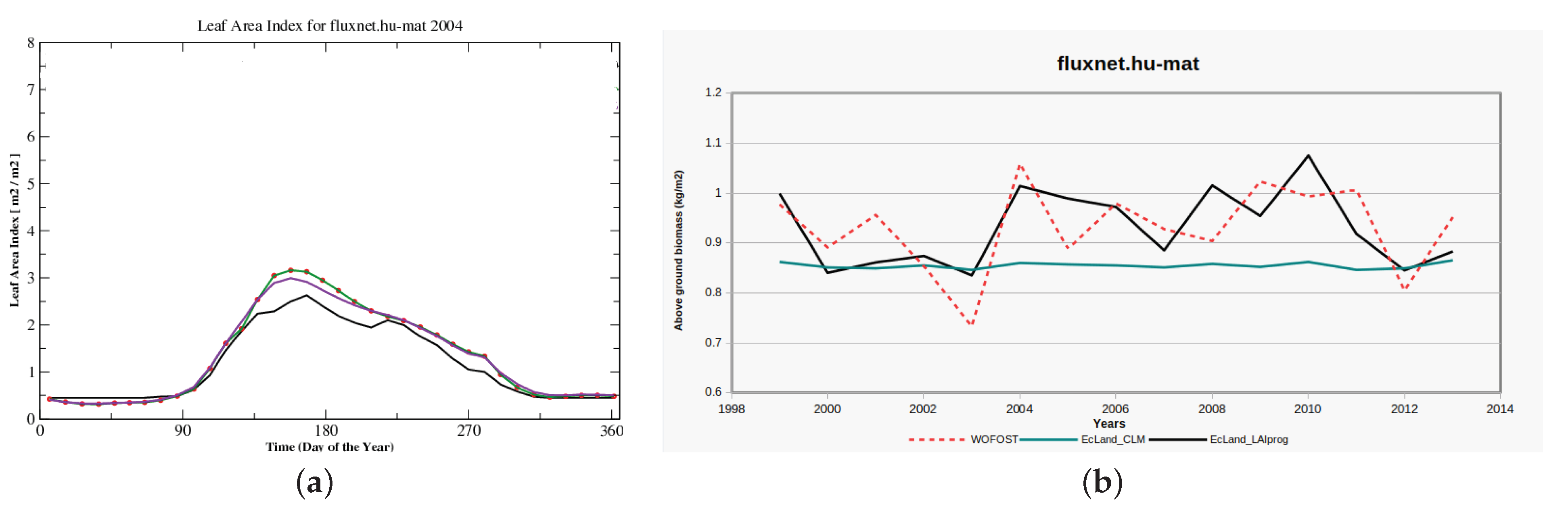
4.2.3. FLUXNET
4.2.4. WOFOST
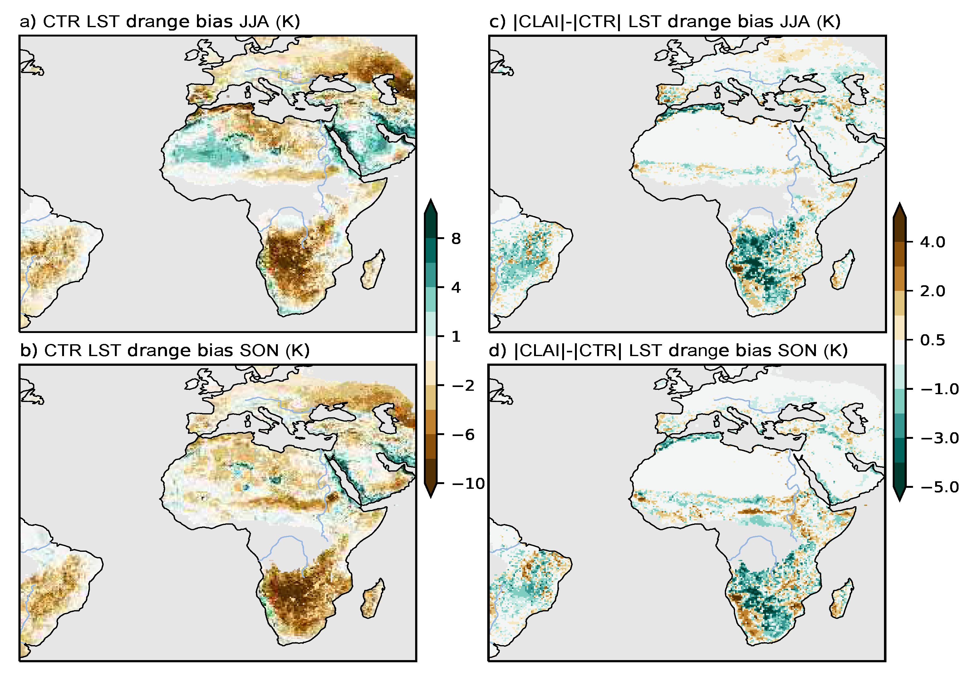
4.2.5. LSA SAF LST
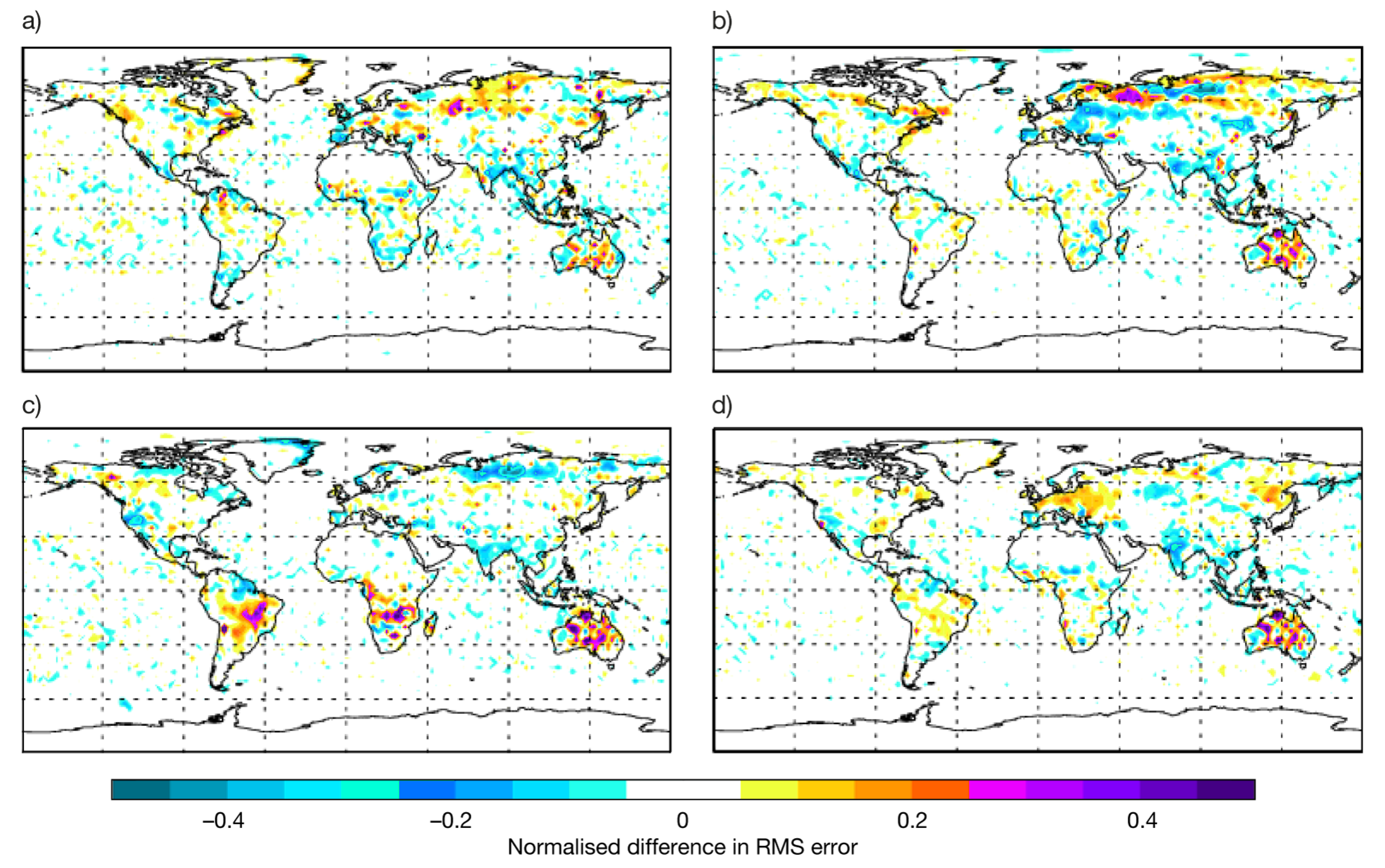
4.2.6. ESA-CCI Soil Moisture
4.2.7. ESM-SnowMIP
4.2.8. SYNOP Observations
4.3. Evaluation of Updated Land Cover and Vegetation
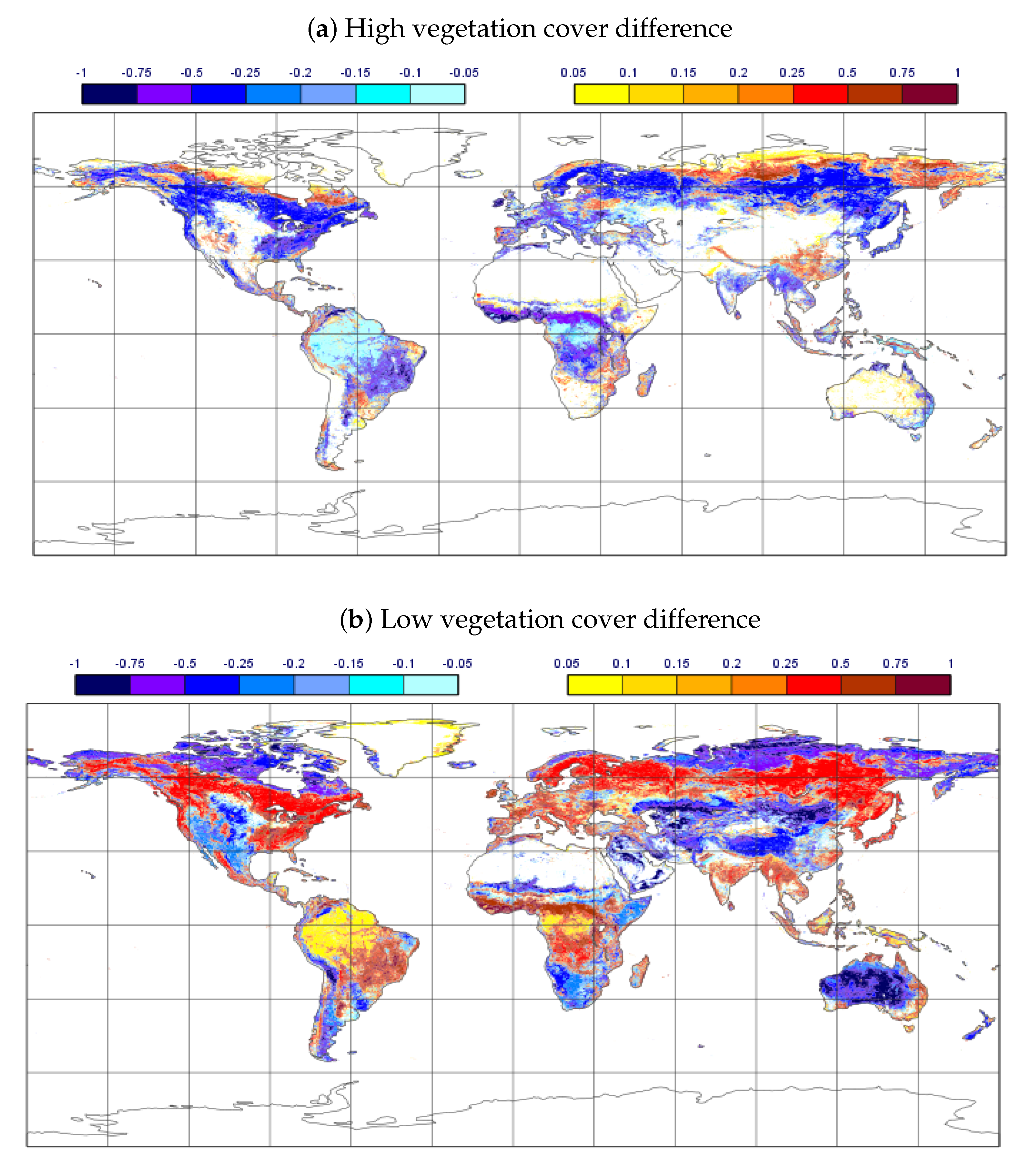
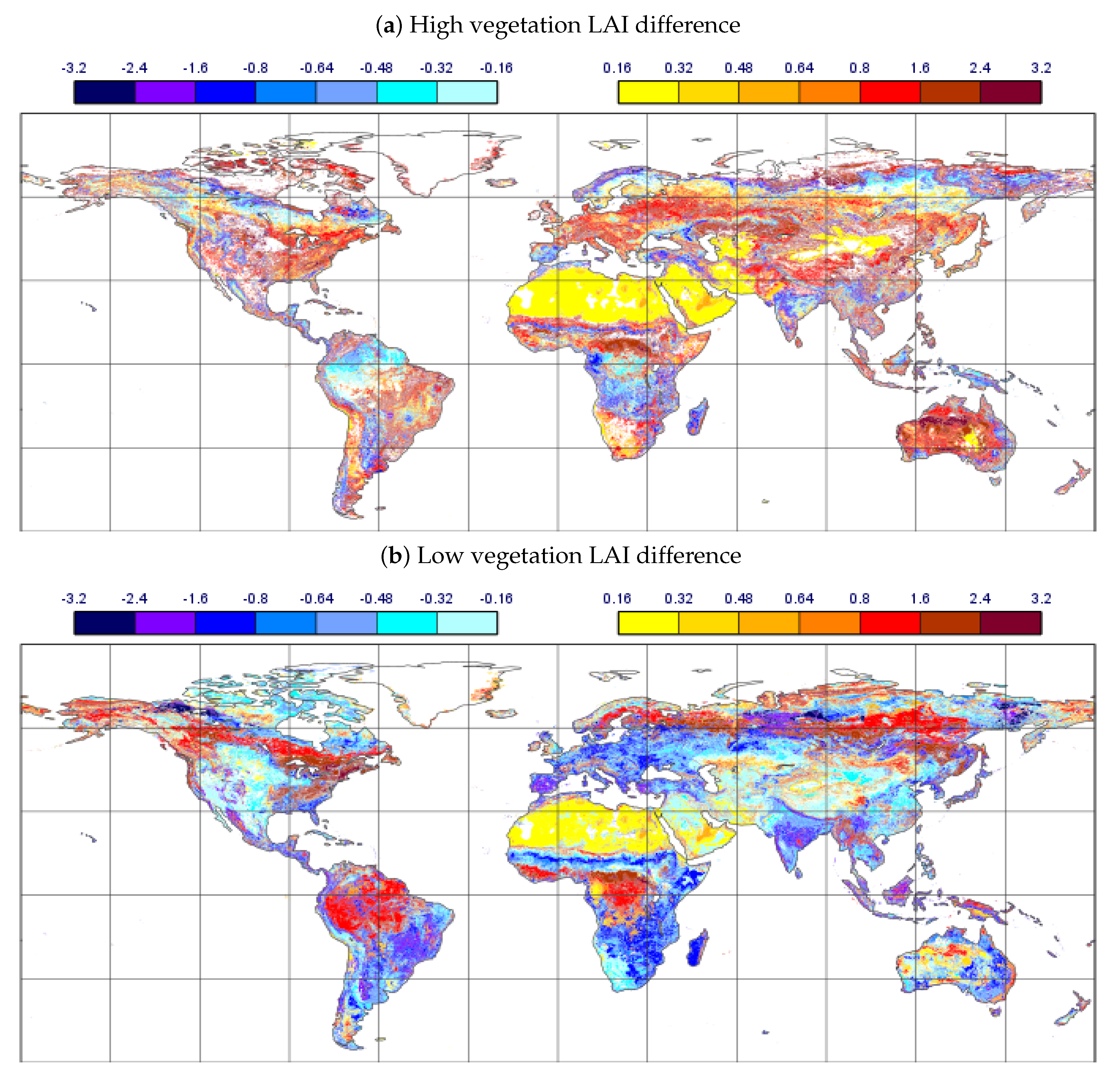
4.3.1. Land Use/Land Cover and Leaf Area Index Evaluation
4.3.2. Evaluation of Dynamic Vegetation
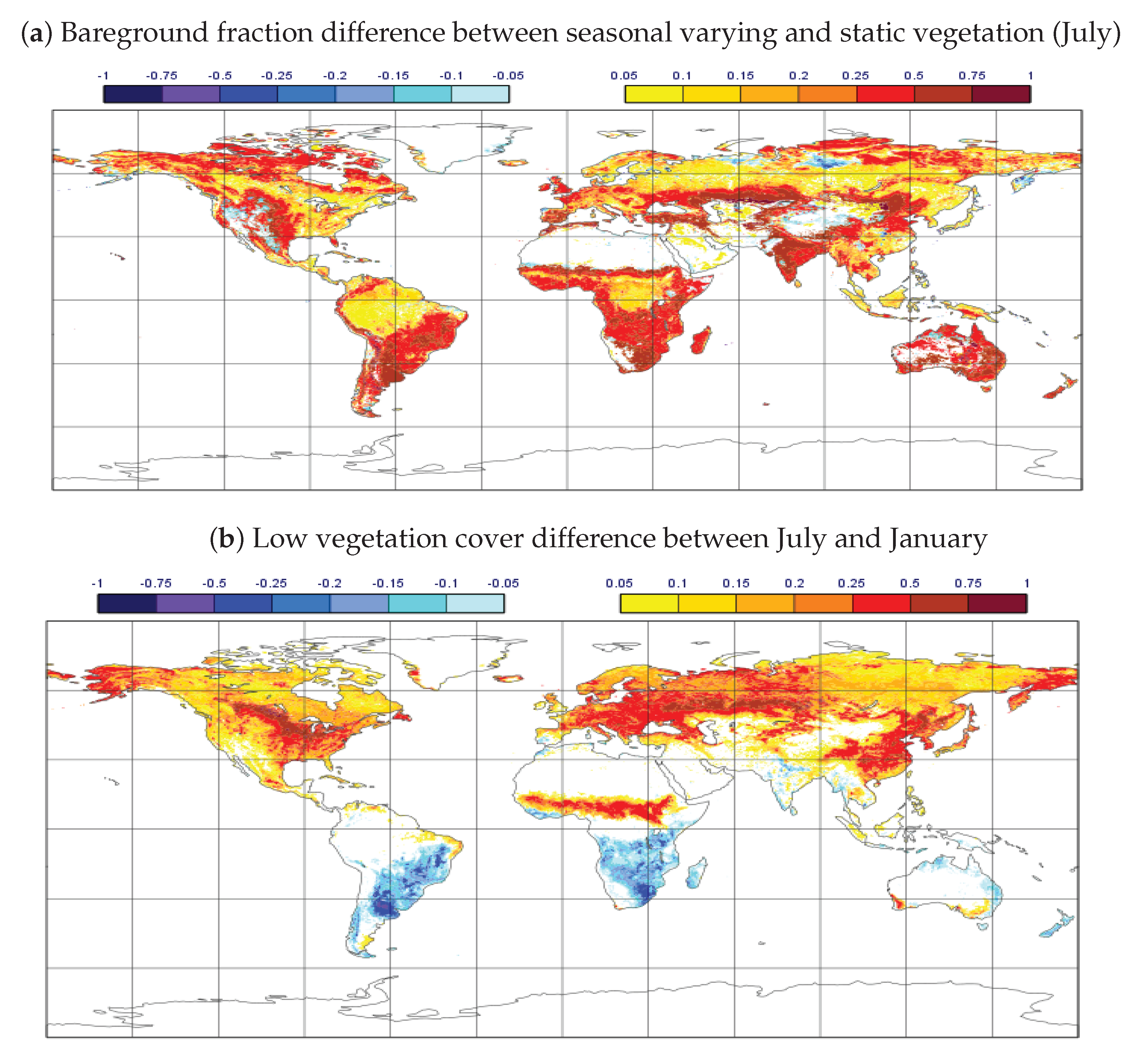
Seasonal Vegetation Cover Evaluation
Prognostic Vegetation Phenology Evaluation
4.4. Evaluation of Updated Snow
4.4.1. Site Evaluation at ESM-SnowMIP
4.4.2. Global Offline Evaluation of the Snow Depth
4.4.3. Global Coupled Evaluation
4.5. Evaluation of Updated Soil Parametrization
4.6. Evaluation of the Updated Surface Water
4.7. Evaluation of Coupled River Discharge
4.8. Evaluation of Urban Representation
5. Summary and Perspectives
Supplementary Materials
Author Contributions
Funding
Acknowledgments
Conflicts of Interest
References
- Best, M.J.; Pryor, M.; Clark, D.B.; Rooney, G.G.; Essery, R.L.H.; Ménard, C.B.; Edwards, J.M.; Hendry, M.A.; Porson, A.; Gedney, N.; et al. The Joint UK Land Environment Simulator (JULES), model description—Part 1: Energy and water fluxes. Geosci. Model. Dev. 2011, 4, 677–699. [Google Scholar] [CrossRef]
- Clark, D.B.; Mercado, L.M.; Sitch, S.; Jones, C.D.; Gedney, N.; Best, M.J.; Pryor, M.; Rooney, G.G.; Essery, R.L.H.; Blyth, E.; et al. The Joint UK Land Environment Simulator (JULES), model description—Part 2: Carbon fluxes and vegetation dynamics. Geosci. Model. Dev. 2011, 4, 701–722. [Google Scholar] [CrossRef]
- Masson, V.; Le Moigne, P.; Martin, E.; Faroux, S.; Alias, A.; Alkama, R.; Belamari, S.; Barbu, A.; Boone, A.; Bouyssel, F.; et al. The SURFEXv7.2 land and ocean surface platform for coupled or offline simulation of earth surface variables and fluxes. Geosci. Model. Dev. 2013, 6, 929–960. [Google Scholar] [CrossRef]
- Lawrence, D.M.; Fisher, R.A.; Koven, C.D.; Oleson, K.W.; Swenson, S.C.; Bonan, G.; Collier, N.; Ghimire, B.; van Kampenhout, L.; Kennedy, D.; et al. The Community Land Model Version 5: Description of New Features, Benchmarking, and Impact of Forcing Uncertainty. J. Adv. Model. Earth Syst. 2019, 11, 4245–4287. [Google Scholar] [CrossRef]
- Van den Hurk, B.J.J.M.; Viterbo, P.; Beljaars, A.C.M.; Betts, A.K. Offline Validation of the ERA40 Surface Scheme; ECMWF Tech. Memo; European Centre for Medium-Range Weather Forecasts: Reading, UK, 2000; Volume 295. [Google Scholar] [CrossRef]
- Viterbo, P.; Beljaars, A.C.M. An Improved Land Surface Parametrization Scheme in the ECMWF Model and Its Validation; ECMWF Tech. Report No. 75; ECMWF Research Department: Reading, UK, 1995. [Google Scholar]
- Viterbo, P.; Beljaars, A.C.M.; Mahouf, J.F.; Teixeira, J. The representation of soil moisture freezing and its impact on the stable boundary layer. Q. J. R. Meteorol. Soc. 1999, 125, 2401–2426. [Google Scholar] [CrossRef]
- Balsamo, G.; Viterbo, P.; Beljaars, A.; van den Hurk, B.; Hirschi, M.; Betts, A.K.; Scipal, K. A revised hydrology for the ECMWF model: Verification from field site to terrestrial water storage and impact in the Integrated Forecast System. J. Hydrometeorol. 2009, 10, 623–643. [Google Scholar] [CrossRef]
- Dutra, E.; Balsamo, G.; Viterbo, P.; Miranda, P.; Beljaars, A.; Schär, C.; Elder, K. An improved snow scheme for the ECMWF Land Surface Model: Description and offline validation. J. Hydrometeorol. 2010, 11, 7499–7506. [Google Scholar] [CrossRef]
- Boussetta, S.; Balsamo, G.; Beljaars, A.; Kral, T.; Jarlan, L. Impact of a satellite-derived Leaf Area Index monthly climatology in a global Numerical Weather Prediction model. Int. J. Rem. Sens. 2013, 34, 3520–3542. [Google Scholar] [CrossRef]
- Uppala, S.M.; KÅllberg, P.W.; Simmons, A.J.; Andrae, U.; Bechtold, V.D.C.; Fiorino, M.; Gibson, J.K.; Haseler, J.; Hernandez, A.; Kelly, G.A.; et al. The ERA-40 re-analysis. Q. J. R. Meteorol. Soc. 2005, 131, 2961–3012. [Google Scholar] [CrossRef]
- Dee, D.P.; Uppala, S.M.; Simmons, A.J.; Berrisford, P.; Poli, P.; Kobayashi, S.; Andrae, U.; Balmaseda, M.A.; Balsamo, G.; Bauer, P.; et al. The ERA-Interim reanalysis: Configuration and performance of the data assimilation system. Q. J. R. Meteorol. Soc. 2011, 137, 553–597. [Google Scholar] [CrossRef]
- Hersbach, H.; Bell, B.; Berrisford, P.; Hirahara, S.; Horányi, A.; Muñoz-Sabater, J.; Nicolas, J.; Peubey, C.; Radu, R.; Schepers, D.; et al. The ERA5 global reanalysis. Q. J. Roy. Meteor. Soc. 2020. [Google Scholar] [CrossRef]
- Muñoz Sabater, J.; Dutra, E.; Agustí-Panareda, A.; Albergel, C.; Arduini, G.; Balsamo, G.; Boussetta, S.; Choulga, M.; Harrigan, S.; Hersbach, H.; et al. ERA5-Land: A state-of-the-art global reanalysis dataset for land applications. Earth Syst. Sci. Data Discuss. 2021, 2021, 1–50. [Google Scholar] [CrossRef]
- Weisheimer, A.; Doblas-Reyes, F.J.; Jung, T.; Palmer, T.N. On the predictability of the extreme summer 2003 over Europe. Geophys. Res. Lett. 2011, 38. [Google Scholar] [CrossRef]
- Dutra, E.; Viterbo, P.; Miranda, P.M.; Balsamo, G. Complexity of snow schemes in a climate model and its impact on surface energy and hydrology. J. Hydrometeorol. 2012, 13, 521–538. [Google Scholar] [CrossRef]
- Mahfouf, J.F.; Noilhan, J. Comparative study of various formulations from bare soil using in situ data. J. Appl. Meteorol. 1991, 30, 1345–1365. [Google Scholar] [CrossRef]
- Agustí-Panareda, A.; Balsamo, G.; Beljaars, A. Impact of improved soil moisture on the ECMWF precipitation forecast in West Africa. Geophys. Res. Lett. 2010, 37. [Google Scholar] [CrossRef]
- Balsamo, G.; Agusti-Panareda, A.; Albergel, C.; Arduini, G.; Beljaars, A.; Bidlot, J.; Blyth, E.; Bousserez, N.; Boussetta, S.; Brown, A.; et al. Satellite and In Situ Observations for Advancing Global Earth Surface Modelling: A Review. Remote Sens. 2018, 10, 38. [Google Scholar] [CrossRef]
- Reichstein, M.; Camps-Valls, G.; Stevens, B.; Jung, M.; Denzler, J.; Carvalhais, N. Deep learning and process understanding for data-driven Earth system science. Nature 2019, 566, 195–204. [Google Scholar] [CrossRef] [PubMed]
- Best, M.J.; Abramowitz, G.; Johnson, H.R.; Pitman, A.J.; Balsamo, G.; Boone, A.; Cuntz, M.; Decharme, B.; Dirmeyer, P.A.; Dong, J.; et al. The Plumbing of Land Surface Models: Benchmarking Model Performance. J. Hydrometeorol. 2015, 16, 1425–1442. [Google Scholar] [CrossRef]
- Haughton, N.; Abramowitz, G.; Pitman, A.J.; Or, D.; Best, M.J.; Johnson, H.R.; Balsamo, G.; Boone, A.; Cuntz, M.; Decharme, B.; et al. The Plumbing of Land Surface Models: Is Poor Performance a Result of Methodology or Data Quality? J. Hydrometeorol. 2016, 17, 1705–1723. [Google Scholar] [CrossRef]
- Schellekens, J.; Dutra, E.; Martínez-de la Torre, A.; Balsamo, G.; van Dijk, A.; Sperna Weiland, F.; Minvielle, M.; Calvet, J.C.; Decharme, B.; Eisner, S.; et al. A global water resources ensemble of hydrological models: The eartH2Observe Tier-1 dataset. Earth Syst. Sci. Data 2017, 9, 389–413. [Google Scholar] [CrossRef]
- Balsamo, G.; Albergel, C.; Beljaars, A.; Boussetta, S.; Brun, E.; Cloke, H.; Dee, D.; Dutra, E.; Muñoz Sabater, J.; Pappenberger, F.; et al. ERA-Interim/Land: A global land surface reanalysis data set. Hydrol. Earth Syst. Sci. 2015, 19, 389–407. [Google Scholar] [CrossRef]
- Balsamo, G.; Engelen, R.; Thiemert, D.; Agustì-Panareda, A.; Bousserez, N.; Broquet, G.; Brunner, D.; Buchwitz, M.; Chevallier, F.; Choulga, M.; et al. The CO2 Human Emissions (CHE) project: First steps towards a European operational capacity to monitor anthropogenic CO2 emissions. Geosci. Model Dev. 2021. Submitted. [Google Scholar]
- Sandu, I.; Haiden, T.; Balsamo, G.; Schmederer, P.; Arduini, G.; Day, J.; Beljaars, A.; Ben-Bouallegue, Z.; Boussetta, S.; Leutbecher, M.; et al. Addressing near-surface forecast biases: Outcomes of the ECMWF project ‘Understanding uncertainties in surface atmosphere exchange’ (USURF). ECMWF Tech. Memo 2020, 875. [Google Scholar] [CrossRef]
- Best, M.J.; Beljaars, A.C.M.; Polcher, J.; Viterbo, P. A proposed structure for coupling tiled surfaces with the planetary boundary layer. J. Hydrol. Meteorol. 2004, 5, 1271–1278. [Google Scholar] [CrossRef]
- Balsamo, G.; Pappenberger, F.; Dutra, E.; Viterbo, P.; van den Hurk, B. A revised land hydrology in the ECMWF model: A step towards daily water flux prediction in a fully-closed water cycle. Hydrol. Process. 2011, 25, 1046–1054. [Google Scholar] [CrossRef]
- Albergel, C.; Balsamo, G.; de Rosnay, P.; Muñoz Sabater, J.; Boussetta, S. A bare ground evaporation revision in the ECMWF land-surface scheme: Evaluation of its impact using ground soil moisture and satellite microwave data. Hydrol. Earth Syst. Sci. 2012, 16, 3607–3620. [Google Scholar] [CrossRef]
- Boussetta, S.; Balsamo, G.; Beljaars, A.; Agusti-Panareda, A.; Calvet, J.; Jacobs, C.; van den Hurk, B.; Viterbo, P.; Lafont, S.; Dutra, E.; et al. Natural land carbon dioxide exchanges in the ECMWF Integrated Forecasting System: Implementation and offline validation. J. Geophys. Res. 2013, 118, 5923–5946. [Google Scholar] [CrossRef]
- Dutra, E.; Stepanenko, V.M.; Balsamo, G.; Viterbo, P.; Miranda, P.M.A.; Mironov, D.; Schär, C. An offline study of the impact of lakes on the performance of the ECMWF surface scheme. Boreal Environ. Res. 2010, 15, 100–112. [Google Scholar]
- Balsamo, G.; Salgado, R.; Dutra, E.; Boussetta, S.; Stockdale, T.; Potes, M. On the contribution of lakes in predicting near-surface temperature in a global weather forecasting model. Tellus A 2012, 64, 15829. [Google Scholar] [CrossRef]
- Balsamo, G. Interactive Lakes in the Integrated Forecasting System; ECMWF Newsletter No. 137; ECMWF: Reading, UK, 2013; pp. 30–34. Available online: https://www.ecmwf.int/en/elibrary/14579-newsletter-no-137-autumn-2013 (accessed on 4 June 2021).
- Loveland, T.R.; Reed, B.C.; Brown, J.F.; Ohlen, D.O.; Zhu, Z.; Youing, L.; Merchant, J.W. Development of a global land cover characteristics database and IGB6 DISCover from the 1 km AVHRR data. Int. J. Remote Sens. 2000, 21, 1303–1330. [Google Scholar] [CrossRef]
- Boussetta, S.; Balsamo, G.; Dutra, E.; Beljaars, A.; Albergel, C. Assimilation of surface albedo and vegetation states from satellite observations and their impact on numerical weather prediction. Remote Sens. Environ. 2015, 163, 111–126. [Google Scholar] [CrossRef]
- Anderson, M.C.; Norman, J.M.; Kustas, W.P.; Li, F.; Prueger, J.H.; Mecikalski, J.R. Effects of Vegetation Clumping on Two–Source Model Estimates of Surface Energy Fluxes from an Agricultural Landscape during SMACEX. J. Hydrometeorol. 2005, 6, 892–909. [Google Scholar] [CrossRef]
- Nogueira, M.; Albergel, C.; Boussetta, S.; Johannsen, F.; Trigo, I.F.; Ermida, S.L.; Martins, J.P.A.; Dutra, E. Role of vegetation in representing land surface temperature in the CHTESSEL (CY45R1) and SURFEX-ISBA (v8.1) land surface models: A case study over Iberia. Geosci. Model. Dev. 2020, 13, 3975–3993. [Google Scholar] [CrossRef]
- Gibelin, A.L.; Calvet, J.C.; Roujean, J.L.; Jarlan, L.; Los, S.O. Ability of the land surface model ISBA-A-gs to simulate leaf area index at the global scale: Comparison with satellites products. J. Geophys. Res. Atmos. 2006, 111. [Google Scholar] [CrossRef]
- Calvet, J.C.; Soussana, J.F. Modelling CO2-enrichment effects using an interactive vegetation SVAT scheme. Agric. For. Meteorol. 2001, 108, 129–152. [Google Scholar] [CrossRef]
- Boone, A.; Etchevers, P. An intercomparison of three snow schemes of varying complexity coupled to the same land surface model: Local-scale evaluation at an alpine site. J. Hydrometeorol. 2001, 2, 374–394. [Google Scholar] [CrossRef]
- Arduini, G.; Balsamo, G.; Dutra, E.; Day, J.J.; Sandu, I.; Boussetta, S.; Haiden, T. Impact of a Multi-Layer Snow Scheme on Near-Surface Weather Forecasts. J. Adv. Model. Earth Syst. 2019, 11, 4687–4710. [Google Scholar] [CrossRef]
- Jordan, R. A One-Dimensional Temperature Model for a Snow Cover: Technical Documentation for SNTHERM; Technical Report CRREL Special Rep. 91-b; Cold Regions Research and Engineering Lab.: Hanover, NH, USA, 1991. [Google Scholar]
- Calonne, N.; Flin, F.; Morin, S.; Lesaffre, B.; du Roscoat, S.R.; Geindreau, C. Numerical and experimental investigations of the effective thermal conductivity of snow. Geophys. Res. Lett. 2011, 38. [Google Scholar] [CrossRef]
- Sun, S.; Jin, J.; Xue, Y. A simple snow-atmosphere-soil transfer model. J. Geophys. Res. Atmos. 1999, 104, 19587–19597. [Google Scholar] [CrossRef]
- Brun, E.; Martin, E.; Spiridonov, V. Coupling a multi-layered snow model with a GCM. Ann. Glaciol. 1997, 25, 66–72. [Google Scholar] [CrossRef]
- Decharme, B.; Brun, E.; Boone, A.; Delire, C.; Le Moigne, P.; Morin, S. Impacts of snow and organic soils parameterization on northern Eurasian soil temperature profiles simulated by the ISBA land surface model. Cryosphere 2016, 10, 853–877. [Google Scholar] [CrossRef]
- Lawrence, D.M.; Slater, A.G.; Romanovsky, V.E.; Nicolsky, D.J. Sensitivity of a model projection of near-surface permafrost degradation to soil column depth and representation of soil organic matter. J. Geophys. Res. Earth Surf. 2008, 113. [Google Scholar] [CrossRef]
- Stevens, D.; Miranda, P.M.A.; Orth, R.; Boussetta, S.; Balsamo, G.; Dutra, E. Sensitivity of Surface Fluxes in the ECMWF Land Surface Model to the Remotely Sensed Leaf Area Index and Root Distribution: Evaluation with Tower Flux Data. Atmosphere 2020, 11, 1362. [Google Scholar] [CrossRef]
- Egea, G.; Verhoef, A.; Vidale, P.L. Towards an improved and more flexible representation of water stress in coupled photosynthesis-stomatal conductance models. Agric. For. Meteorol. 2011, 151, 1370–1384. [Google Scholar] [CrossRef]
- Verhoef, A.; Egea, G. Modeling plant transpiration under limited soil water: Comparison of different plant and soil hydraulic parameterizations and preliminary implications for their use in land surface models. Agric. For. Meteorol. 2014, 191, 22–32. [Google Scholar] [CrossRef]
- Orth, R.; Dutra, E.; Pappenberger, F. Improving weather predictability by including land surface model parameter uncertainty. Mon. Weather Rev. 2016, 144, 1551–1569. [Google Scholar] [CrossRef]
- Samaniego, L.; Kumar, R.; Attinger, S. Multiscale parameter regionalization of a grid-based hydrologic model at the mesoscale. Water Resour. Res. 2010, 46. [Google Scholar] [CrossRef]
- Choulga, M.; Kourzeneva, E.; Balsamo, G.; Boussetta, S.; Wedi, N. Upgraded global mapping information for earth system modelling: An application to surface water depth at the ECMWF. Hydrol. Earth Syst. Sci. 2019, 23, 4051–4076. [Google Scholar] [CrossRef]
- Alfieri, L.; Burek, P.; Dutra, E.; Krzeminski, B.; Muraro, D.; Thielen, J.; Pappenberger, F. GloFAS-global ensemble streamflow forecasting and flood early warning. Hydrol. Earth Syst. Sci. 2013, 17, 1161–1175. [Google Scholar] [CrossRef]
- Voldoire, A.; Decharme, B.; Pianezze, J.; Lebeaupin Brossier, C.; Sevault, F.; Seyfried, L.; Garnier, V.; Bielli, S.; Valcke, S.; Alias, A.; et al. SURFEX v8.0 interface with OASIS3-MCT to couple atmosphere with hydrology, ocean, waves and sea-ice models, from coastal to global scales. Geosci. Model. Dev. 2017, 10, 4207–4227. [Google Scholar] [CrossRef]
- Zsóter, E.; Cloke, H.; Stephens, E.; de Rosnay, P.; Muñoz-Sabater, J.; Prudhomme, C.; Pappenberger, F. How well do operational numerical weather prediction configurations represent hydrology? J. Hydrometeorol. 2019, 20, 1533–1552. [Google Scholar] [CrossRef]
- Zuo, H.; de Boisseson, E.; Zsoter, E.; Harrigan, S.; de Rosnay, P.; Wetterhall, F.; Prudhomme, C. Benefits of Dynamically Modelled River Discharge Input for Ocean and Coupled System. EGU General Assembly Conference Abstracts. 2020, p. 8564. Available online: https://ui.adsabs.harvard.edu/abs/2020EGUGA..22.8564Z/abstract (accessed on 17 April 2021).
- Bates, P.D.; Horritt, M.S.; Fewtrell, T.J. A simple inertial formulation of the shallow water equations for efficient two-dimensional flood inundation modelling. J. Hydrol. 2010, 387, 33–45. [Google Scholar] [CrossRef]
- Yamazaki, D.; Kanae, S.; Kim, H.; Oki, T. A physically based description of floodplain inundation dynamics in a global river routing model. Water Resour. Res. 2011, 47, W04501. [Google Scholar] [CrossRef]
- Yamazaki, D.; De Almeida, G.A.; Bates, P.D. Improving computational efficiency in global river models by implementing the local inertial flow equation and a vector-based river network map. Water Resour. Res. 2013, 49, 7221–7235. [Google Scholar] [CrossRef]
- Yamazaki, D.; O’Loughlin, F.; Trigg, M.A.; Miller, Z.F.; Pavelsky, T.M.; Bates, P.D. Development of the Global Width Database for Large Rivers. Water Resour. Res. 2014, 50. [Google Scholar] [CrossRef]
- Yamazaki, D.; Lee, H.; Alsdorf, D.E.; Dutra, E.; Kim, H.; Kanae, S.; Oki, T. Analysis of the water level dynamics simulated by a global river model: A case study in the Amazon River. Water Resour. Res. 2012, 48, W09508. [Google Scholar] [CrossRef]
- Decharme, B.; Delire, C.; Minvielle, M.; Colin, J.; Vergnes, J.P.; Alias, A.; Saint-Martin, D.; Séférian, R.; Sénési, S.; Voldoire, A. Recent Changes in the ISBA-CTRIP Land Surface System for Use in the CNRM-CM6 Climate Model and in Global Off-Line Hydrological Applications. J. Adv. Model. Earth Syst. 2019, 11, 1207–1252. [Google Scholar] [CrossRef]
- Yamazaki, D.; Ikeshima, D.; Sosa, J.; Bates, P.D.; Allen, G.H.; Pavelsky, T.M. MERIT Hydro: A High-Resolution Global Hydrography Map Based on Latest Topography Dataset. Water Resour. Res. 2019, 55, 5053–5073. [Google Scholar] [CrossRef]
- Yamazaki, D.; Ikeshima, D.; Tawatari, R.; Yamaguchi, T.; O’Loughlin, F.; Neal, J.C.; Sampson, C.C.; Kanae, S.; Bates, P.D. A high-accuracy map of global terrain elevations. Geophys. Res. Lett. 2017, 44. [Google Scholar] [CrossRef]
- Yamazaki, D.; Sato, T.; Kanae, S.; Hirabayashi, Y.; Bates, P.D. Regional flood dynamics in a bifurcating mega delta simulated in a global river model. Geophys. Res. Lett. 2014, 41. [Google Scholar] [CrossRef]
- Yamazaki, D.; Trigg, M.A.; Ikeshima, D. Development of a global ∼90 m water body map using multi-temporal Landsat images. Remote Sens. Environ. 2015, 171. [Google Scholar] [CrossRef]
- Mogensen, K.; Keeley, S.; Towers, P. Coupling of the NEMO and IFS models in a single executable. ECMWF Tech. Memo 2012, 673, 1–25. [Google Scholar] [CrossRef]
- McNorton, J.; Arduini, G.; Bousserez, N.; Agustí-Panareda, A.; Balsamo, G.; Boussetta, S.; Choulga, M.; Hadade, I.; Hogan, R. An Urban Scheme for the ECMWF Integrated Forecasting System: Single-Column and Global Offline Application. J. Adv. Model. Earth Syst. 2021, 4. [Google Scholar] [CrossRef]
- Masson, V. A physically-based scheme for the urban energy budget in atmospheric models. Bound. Layer Meteorol. 2000, 94, 357–397. [Google Scholar] [CrossRef]
- Oleson, K.W.; Bonan, G.B.; Feddema, J.; Vertenstein, M. An urban parameterization for a global climate model. Part II: Sensitivity to input parameters and the simulated urban heat island in offline simulations. J. Appl. Meteorol. Climatol. 2008, 47, 1061–1076. [Google Scholar] [CrossRef]
- Porson, A.; Clark, P.A.; Harman, I.; Best, M.; Belcher, S. Implementation of a new urban energy budget scheme in the MetUM. Part I: Description and idealized simulations. Q. J. R. Meteorol. Soc. 2010, 136, 1514–1529. [Google Scholar] [CrossRef]
- Faroux, S.; Kaptué Tchuenté, A.; Roujean, J.L.; Masson, V.; Martin, E.; Moigne, P.L. ECOCLIMAP-II/Europe: A twofold database of ecosystems and surface parameters at 1 km resolution based on satellite information for use in land surface, meteorological and climate models. Geosci. Model. Dev. 2013, 6, 563–582. [Google Scholar] [CrossRef]
- Wedi, N.P.; Polichtchouk, I.; Dueben, P.; Anantharaj, V.G.; Bauer, P.; Boussetta, S.; Browne, P.; Deconinck, W.; Gaudin, W.; Hadade, I.; et al. A Baseline for Global Weather and Climate Simulations at 1 km Resolution. J. Adv. Model. Earth Syst. 2020, 12, e2020MS002192. [Google Scholar] [CrossRef]
- Bauer, P.; Quintino, T.; Wedi, N.; Bonanni, A.; Chrust, M.; Deconinck, W.; Diamantakis, M.; Düben, P.; English, S.; Flemming, J.; et al. The ECMWF Scalability Programme: Progress and Plans. ECMWF Tech. Memo 2020, 857. [Google Scholar] [CrossRef]
- Jung, M.; Schwalm, C.; Migliavacca, M.; Walther, S.; Camps-Valls, G.; Koirala, S.; Anthoni, P.; Besnard, S.; Bodesheim, P.; Carvalhais, N.; et al. Scaling carbon fluxes from eddy covariance sites to globe: Synthesis and evaluation of the FLUXCOM approach. Biogeosciences 2020, 17, 1343–1365. [Google Scholar] [CrossRef]
- Miralles, D.G.; Holmes, T.R.H.; de Jeu, R.A.M.; Gash, J.H.; Meesters, A.G.C.A.; Dolman, A.J. Global land-surface evaporation estimated from satellite-based observations. Hydrol. Earth Syst. Sci. 2011, 15, 453–469. [Google Scholar] [CrossRef]
- Martens, B.; Miralles, D.G.; Lievens, H.; Van Der Schalie, R.; De Jeu, R.A.; Fernández-Prieto, D.; Beck, H.E.; Dorigo, W.A.; Verhoest, N.E.C. GLEAM v3: Satellite-based land evaporation and root-zone soil moisture. Geosci. Model. Dev. 2017, 10, 1903–1925. [Google Scholar] [CrossRef]
- Baldocchi, D.; Falge, E.; Gu, L.; Olson, R.; Hollinger, D.; Running, S.; Anthoni, P.; Bernhofer, C.; Davis, K.; Evans, R.; et al. FLUXNET: A New Tool to Study the Temporal and Spatial Variability of Ecosystem-Scale Carbon Dioxide, Water Vapor, and Energy Flux Densities. Bull. Am. Meteorol. Soc. 2001, 82, 2415–2434. [Google Scholar] [CrossRef]
- Reichstein, M.; Falge, E.; Baldocchi, D.; Papale, D.; Aubinet, M.; Berbigier, P.; Bernhofer, C.; Buchmann, N.; Gilmanov, T.; Granier, A.; et al. On the separation of net ecosystem exchange into assimilation and ecosystem respiration: Review and improved algorithm. Glob. Chang. Biol. 2005, 11, 1424–1439. [Google Scholar] [CrossRef]
- Freitas, S.C.; Trigo, I.F.; Bioucas-Dias, J.M.; Gottsche, F. Quantifying the Uncertainty of Land Surface Temperature Retrievals From SEVIRI/Meteosat. IEEE Trans. Geosci. Remote Sens. 2010, 48, 523–534. [Google Scholar] [CrossRef]
- Johannsen, F.; Ermida, S.; Martins, J.P.A.; Trigo, I.F.; Nogueira, M.; Dutra, E. Cold Bias of ERA5 Summertime Daily Maximum Land Surface Temperature over Iberian Peninsula. Remote Sens. 2019, 11, 2570. [Google Scholar] [CrossRef]
- Gruber, A.; Scanlon, T.; van der Schalie, R.; Wagner, W.; Dorigo, W. Evolution of the ESA CCI Soil Moisture climate data records and their underlying merging methodology. Earth Syst. Sci. Data 2019, 11, 717–739. [Google Scholar] [CrossRef]
- Dorigo, W.; Wagner, W.; Albergel, C.; Albrecht, F.; Balsamo, G.; Brocca, L.; Chung, D.; Ertl, M.; Forkel, M.; Gruber, A.; et al. ESA CCI Soil Moisture for improved Earth system understanding: State-of-the art and future directions. Remote Sens. Environ. 2017, 203, 185–215. [Google Scholar] [CrossRef]
- Gruber, A.; Dorigo, W.A.; Crow, W.; Wagner, W. Triple Collocation-Based Merging of Satellite Soil Moisture Retrievals. IEEE Trans. Geosci. Remote Sens. 2017, 55, 6780–6792. [Google Scholar] [CrossRef]
- Ménard, C.B.; Essery, R.; Barr, A.; Bartlett, P.; Derry, J.; Dumont, M.; Fierz, C.; Kim, H.; Kontu, A.; Lejeune, Y.; et al. Meteorological and evaluation datasets for snow modelling at 10 reference sites: Description of in situ and bias-corrected reanalysis data. Earth Syst. Sci. Data 2019, 11, 865–880. [Google Scholar] [CrossRef]
- Haiden, T.; Janousek, M.; Bidlot, J.; Buizza, R.; Ferranti, L.; Prates, F.; Vitart, F. Evaluation of ECMWF Forecasts, Including the 2018 Upgrade; European Centre for Medium Range Weather Forecasts: Readubf, UK, 2018. [Google Scholar]
- Nogueira, M.; Boussetta, S.; Balsamo, G.; Albergel, C.; Trigo, I.F.; Johannsen, S.L.; Miralles, D.; Dutra, E. Upgrading land-cover and vegetation seasonality in the ECMWF coupled system: Verification with FLUXNET sites, METEOSAT satellite land surface temperatures and ERA5 atmospheric reanalysis. J. Geophys. Res. 2021. Submitted. [Google Scholar]
- Krinner, G.; Derksen, C.; Essery, R.; Flanner, M.; Hagemann, S.; Clark, M.; Hall, A.; Rott, H.; Brutel-Vuilmet, C.; Kim, H.; et al. ESM-SnowMIP: Assessing snow models and quantifying snow-related climate feedbacks. Geosci. Model. Dev. 2018, 11, 5027–5049. [Google Scholar] [CrossRef]
- De Rosnay, P.; Iseksen, L.; Dahoui, M. Snow data assimilation at ECMWF. ECMWF Newsl. 2015, 143, 26–31. [Google Scholar] [CrossRef]
- Day, J.J.; Arduini, G.; Sandu, I.; Magnusson, L.; Beljaars, A.; Balsamo, G.; Rodwell, M.; Richardson, D. Measuring the impact of a new snow model using surface energy budget process relationships. J. Adv. Model. Earth Syst. 2020, 12, e2020MS002144. [Google Scholar] [CrossRef]
- Bauer, P.; Magnusson, L.; Thépaut, J.N.; Hamill, T.M. Aspects of ECMWF model performance in polar areas. Q. J. R. Meteorol. Soc. 2016, 142, 583–596. [Google Scholar] [CrossRef]
- Moreno-Garcia, M.C. Intensity and form of the urban heat island in Barcelona. Int. J. Climatol. 1994, 14, 705–710. [Google Scholar] [CrossRef]
- Basara, J.B.; Hall, P.K., Jr.; Schroeder, A.J.; Illston, B.G.; Nemunaitis, K.L. Diurnal cycle of the Oklahoma City urban heat island. J. Geophys. Res. Atmos. 2008, 113. [Google Scholar] [CrossRef]
- Hirahara, Y.; Rosnay, P.D.; Arduini, G. Evaluation of a Microwave Emissivity Module for Snow Covered Area with CMEM in the ECMWF Integrated Forecasting System. Remote Sens. 2020, 12, 2946. [Google Scholar] [CrossRef]
- Haiden, T.; Janousek, M.; Vitart, F.; Ben-Bouallegue, Z.; Ferranti, L.; Prates, C.; Richardson, D. Evaluation of ECMWF forecasts, including the 2020 upgrade. ECMWF Tech. Memo 2021, 880. [Google Scholar] [CrossRef]
- Terzago, S.; Andreoli, V.; Arduini, G.; Balsamo, G.; Campo, L.; Cassardo, C.; Cremonese, E.; Dolia, D.; Gabellani, S.; von Hardenberg, J.; et al. Sensitivity of snow models to the accuracy of meteorological forcings in mountain environments. Hydrol. Earth Syst. Sci. 2020, 24, 4061–4090. [Google Scholar] [CrossRef]
- Collier, N.; Hoffman, F.M.; Lawrence, D.M.; Keppel-Aleks, G.; Koven, C.D.; Riley, W.J.; Mu, M.; Randerson, J.T. The International Land Model Benchmarking (ILAMB) System: Design, Theory, and Implementation. J. Adv. Model. Earth Syst. 2018, 10, 2731–2754. [Google Scholar] [CrossRef]
- Baugh, C.; de Rosnay, P.; Lawrence, H.; Jurlina, T.; Drusch, M.; Zsóter, E.; Prudhomme, C. The Impact of SMOS Soil Moisture Data Assimilation within the Operational Global Flood Awareness System (GloFAS). Remote Sens. 2020, 12, 1490. [Google Scholar] [CrossRef]


| Model Development | Experiment Type | Name | Comment |
|---|---|---|---|
| Surface water representation | Offline Surface simulation | OSW | Updated lake parameters |
| Coupled Forecast + Data assimilation | DASW | Updated Glacier, Land water mask and lake | |
| Updated LU/LC and LAI | Offline Surface simulation | CLAI | ESA-CCI land cover and LAI conservative disaggregation |
| Coupled Forecast simulation | FCLAI | ||
| Seasonal vegetation cover | Offline Surface simulation | OSCV | LAI based Seasonal vegetation cover |
| Coupled Forecast simulation | FSCV | ||
| Prognostic LAI | Offline Surface simulation | OPLAI | Prognostic LAI based on daily CO balance |
| New snow multilayers | Offline Surface simulation | OSnML5 | 5 Layers snow scheme |
| Coupled Forecast | FSnML5 | 5 layers scheme | |
| Increased soil depth and discretization | Offline Surface simulation | OSML10_TW | 10 Layers soil 8 m for temperature and water |
| OSML10_T | 10 Layers soil 8 m for temperature and 3 m for water | ||
| Coupling with hydrodynamic | Offline Surface simulation coupled with routing model | - | details in Section 4.7 |
| Urban parametrization | Offline Surface simulation | OSMU | offline 1D and 2D urban parametrization |
| Single Column simulation | SCMU | coupled 1D forecast with urban parametrization |
Publisher’s Note: MDPI stays neutral with regard to jurisdictional claims in published maps and institutional affiliations. |
© 2021 by the authors. Licensee MDPI, Basel, Switzerland. This article is an open access article distributed under the terms and conditions of the Creative Commons Attribution (CC BY) license (https://creativecommons.org/licenses/by/4.0/).
Share and Cite
Boussetta, S.; Balsamo, G.; Arduini, G.; Dutra, E.; McNorton, J.; Choulga, M.; Agustí-Panareda, A.; Beljaars, A.; Wedi, N.; Munõz-Sabater, J.; et al. ECLand: The ECMWF Land Surface Modelling System. Atmosphere 2021, 12, 723. https://doi.org/10.3390/atmos12060723
Boussetta S, Balsamo G, Arduini G, Dutra E, McNorton J, Choulga M, Agustí-Panareda A, Beljaars A, Wedi N, Munõz-Sabater J, et al. ECLand: The ECMWF Land Surface Modelling System. Atmosphere. 2021; 12(6):723. https://doi.org/10.3390/atmos12060723
Chicago/Turabian StyleBoussetta, Souhail, Gianpaolo Balsamo, Gabriele Arduini, Emanuel Dutra, Joe McNorton, Margarita Choulga, Anna Agustí-Panareda, Anton Beljaars, Nils Wedi, Joaquín Munõz-Sabater, and et al. 2021. "ECLand: The ECMWF Land Surface Modelling System" Atmosphere 12, no. 6: 723. https://doi.org/10.3390/atmos12060723
APA StyleBoussetta, S., Balsamo, G., Arduini, G., Dutra, E., McNorton, J., Choulga, M., Agustí-Panareda, A., Beljaars, A., Wedi, N., Munõz-Sabater, J., de Rosnay, P., Sandu, I., Hadade, I., Carver, G., Mazzetti, C., Prudhomme, C., Yamazaki, D., & Zsoter, E. (2021). ECLand: The ECMWF Land Surface Modelling System. Atmosphere, 12(6), 723. https://doi.org/10.3390/atmos12060723