Article

Improved Estimates of the Vertical Structures of Rain Using Single Frequency Doppler Radars

by
Arthur R. Jameson
1,*,
Michael L. Larsen
2 and
David B. Wolff
3
1
RJH Scientific, Inc., El Cajon, CA 92020, USA
2
Department of Physics, College of Charleston, Charleston, SC 29424, USA
3
Wallop’s Island Flight Facility, NASA, Washington, DC 20546, USA
*
Author to whom correspondence should be addressed.
Atmosphere 2021, 12(6), 699; https://doi.org/10.3390/atmos12060699
Submission received: 15 April 2021 / Revised: 18 May 2021 / Accepted: 28 May 2021 / Published: 30 May 2021
(This article belongs to the Section Meteorology)

Abstract

:
It is important to understand the statistical–physical structure of the rain in the vertical so that observations aloft can be translated meaningfully into what will occur at the surface. In order to achieve this understanding, it is necessary to gather high temporal and spatial resolution observations of rain in the vertical. This can be achieved by translating radar Doppler spectra into drop size distributions. A long-standing difficulty in using such measurements, however, is the problem of vertical air motion, which can shift the Doppler spectra and therefore significantly alter the deduced drop size distributions and integrated variables. In this work, we overcome this difficulty by requiring that the measured radar reflectivity and the calculated rainfall rates satisfy fundamental physical theory. As a consequence, the mean vertical airspeed can be estimated and removed. Application of this new approach is demonstrated using vertically pointing Doppler radar observations in weak convection. It is shown that the new approach produces what appear to be better estimates of the rainfall rates as well as estimates of the temporal and spatial regionally coherent updraft and downdrafts occurring in the precipitation. The technique is readily applicable to other radars, especially those operating at non-attenuating frequencies.

1. Introduction

With the development of Doppler radar, it was quickly realized that by pointing the radar antenna vertically, it would be possible to observe the vertical motion of the rain drops reflecting the fall speeds of the drops within updrafts and downdrafts [1], and that this motion could provide estimates of the drop size distributions aloft [2,3]. The reason for this is that the terminal fall speeds of drops are well-known functions of the sizes of the drops [4,5] as well as the altitude of the descent [6]. However, one of the primary difficulties in performing the transformation of Doppler fall speeds into drop sizes is the potential effect of vertical air motion. In downdrafts, for example, a drop of a particular size will move faster toward the radar than when the air is still, leading to an overestimation of its true size.
In an attempt to account for this air motion, two approaches have been proposed. The first was the lower bound method originally suggested by Probert-Jones and Harper [1] and implemented by [7]. Another was that of relating the mean particle fall velocity to the radar reflectivity factor through a power-law [8,9]. Both methods suffer from unproven assumptions. Specifically, the lower bound method assumes that the Doppler spectra coincide with broad distributions of drop sizes containing some of the smallest detectable sizes. If true, then in a sufficiently strong updraft, the fastest moving particles observed moving away from the radar would correspond to the updraft velocity minus the fall speed of the smallest detectable drops (often around 1 m s−1), while in a strong downdraft the slowest moving particles moving toward the radar would correspond to the downdraft velocity plus the fall speed of the smallest drops. The remaining fall speeds are then then assigned to the remaining velocity bins according to their fall speeds. While a logical approach, size sorting of raindrops in convective storms is not unusual, so that there is no guarantee that the drop size distributions are going to be sufficiently broad. In the second power-law-method, the fall speed depends upon the radar reflectivity factor, Z. This is hard to justify since Z also depends upon the drop concentration while fall speeds do not.
In some instances, a direct separation of air motion from rain drop fall speed is possible if one also happens to have simultaneous observations at 94 GHz [10], provided that the signal is not obliterated by attenuation. However, in almost all actual situations, such measurements are not available so that one is left with picking one of the first two choices just discussed above.
In this work, we propose an alternative approach by looking for vertical air speeds which are consistent with both the diameter dependence of the rainfall rate in still air, R, and with the diameter dependence of the backscatter by raindrops at the frequency of the radar, as elaborated on further below. The idea is to use all of the available information. The total measured backscattered power is Pm = C × Zm, where C is a constant associated with the characteristics of the radar, and Zm is then the measured radar reflectivity. However, Zm is also equal to Z m = C η N ( D ) σ ( D ) where Cη is factor related to the radar wavelength, λ, that is described below The Doppler spectrum provides the bridge between theory (Z) and measurements (Zm).
That is, it is well known that drops fall at a velocity determined by its size. This means that in principle, the distribution of these velocities in a Doppler spectrum can be transformed into the distribution of drop sizes, N(D) [11]. However, the vertical air velocity, w, usually alters this distribution of drop fall speeds. In order to compute N(D), then, w must be estimated and removed. As just discussed above, this has been a lingering problem for 60 years. A potential solution when a radar is well-calibrated, though, is to use the additional information provided by the direct measurement of Zm, while the calculated Z can be computed either by circularly shifting the array of drop fall speeds corresponding to each radar velocity bin with the null vertical air speed across the observed Doppler spectrum or alternatively by circularly shifting the Doppler spectrum systematically across a fixed array of drop sizes (fall speeds) to produce Z. By computing different Nob(D,w) for different w one can then search for the w that produces the correct Nob(D,w) = N(D) so that the computed Z = Zm. This is where the Doppler spectra enter, because the spectral power values can be shifted one velocity bin at a time through the entire Nyquist velocity interval of the radar until Z = Zm. The number of velocity bins shifted to achieve this result then provides the estimate of w required to derive N(D). This will become clearer in the next section.
In this particular paper, we focus on the Micro-Rain Radar Pro (MRR), which is a vertical pointing continuous wave radar operating at a frequency of 24.23 GHz and is produced by METEK Corporation. The characteristics, for example, are described in [12]. When the vertical velocities (w) are large enough, they can lead to Doppler spectral aliasing as noted by others (e.g., [13]), but as we show below, the effects of vertical air motion are significant even without aliasing. The important point here is that the MRR calculation of the rainfall rate assumes that the vertical air motion is null on average over long time periods. While that is certainly open to dispute, if one were interested in examining the detailed temporal and spatial structure of rain in the vertical, as we are, such an assumption is not justified.
While the general outline above of the approach applies to most meteorological radars, the MRR data pose additional challenges arising from attenuation by rain at that frequency. Specifically, the MRR processor attempts to account for this attenuation by taking the computed drop size distribution deduced assuming w = 0 and then computing what the attenuation would have been and adjusting the observed Z accordingly. On the other hand, the spectral powers are not adjusted so that when attempting to use them to recompute quantities for w ≠ 0, they will not agree with this corrected Z. Hence, when comparing our computed Z as described below with the MRR adjusted Z, there will be some need to augment the spectral powers when looking for different solutions for different w, as discussed further below. Hence, without an exact knowledge of the attenuation, all results below must be considered estimates, where attenuation is likely to be significant, particularly with increasing altitude.
In the next section we develop the approach for overcoming this difficulty. This is then followed by a section of data analyses applying this approach to MRR Pro data in convective rain provided by the NASA Wallop’s Island precipitation facility.

2. Background

2.1. Basic Considerations

To start this process, we first consider the dependence of the backscatter cross-section of raindrops at the frequency of the MRR for spherical drop diameters (D) over the size range used by the MRR ranging from about 0.077 mm up to 5.13 mm. It is well-known that the scattering at this frequency no longer strictly satisfies the Rayleigh–Gans criteria for a D6 dependence. Nevertheless, the deviations do not appear as severe as often thought. Using cross-sections as computed in [14] (see Appendix A.1), it is clear from Figure 1 that over the indicated range of drop sizes where σB is in cm2 and D is the drop diameter in mm,
σ B = 1.339 × 1 0 4 D 6.083
Note that this power law somewhat over-estimates σB at the largest drop sizes. Such large drops are usually a rarity compared to the prevalence of the other drop sizes, however. Other fits are possible, of course, but tests of a few alternatives show that they do not significantly alter the deduced vertical structures in the rain shown below.
The backscatter power observed by a radar is often expressed using the radar reflectivity η = ∑σB, where the summation is over all of the drops in a unit volume. For a Doppler spectrum, η is then spread over the velocity bins that for our purpose here using the MRR is 64 bins distributed over a range from 0.1858 m s−1 to 11.89 m s−1 depending upon the drop sizes and concentrations at each velocity.
On the other hand, the rainfall rate is the volume flux per unit area and per unit time or simply
R = π 6 D 3 V t ( D )
where Vt(D) is the terminal fall speed of drop of diameter D, and the summation is over all the drops. Often Vt is in m s−1 while D is usually expressed in cm. However, for convenience in this case, D is in mm. Using the relation in [6] (i.e., Vt = −0.193 + 4.96 D − 0.904 D2 + 0.0566 D3, where D is in cm), we consider the combined term D3Vt to yield the relation shown in Figure 2.
The MRR uses two scattering quantities, namely the radar reflectivity as defined above and the equivalent radar reflectivity factor. For Rayleigh scatterers, it is related to what is known as the equivalent radar reflectivity, Z, such that (for example see [15]).
Z = λ 4 π 5 | K | 2 N ( D ) D 6 = 1 C η η
Z = λ 4 π 5 | K | 2 η
where λ is the radar wavelength, and |K|2 is a factor related to the microwave complex index of refraction of the scattering material and is 0.92 for water at most precipitation radar wavelengths. The measured Z is then derived from [15] and more specifically for the MRR radar by
Z = λ 4 π 5 | K | 2 f ( D ) η
where f(D) is the adjustment function accounting for the slight deviations of the raindrop backscatter cross-section from the Rayleigh scatter, as discussed in the MRR literature from the company (“MRR Physical Basics”, p.16 and included in the attached data set). This minor change is included in the development below, so that when we calculate Z later it will be equivalent to the Zm reported by the MRR radar processor.
Now let us consider the distribution functions over drop diameters of the rainfall rate and the radar reflectivity. Then for a particular drop size bin of size ΔD centered on diameter D, it follows from the distribution functions of R and η over D that
Δ R = C R D 3.189 N ( D ) Δ D w h i l e Δ η = C η D 6.08 N ( D ) Δ D
where 1/Cη = 1.339 × 10⁻² when η has units of mm2 m−3 while CR = (π/6)(3.6 × 10−3) × 6.637 = 1.2510 × 10⁻² and R is in mm h−1. We then have
Δ η = C η C R D 2.89 Δ R
so that after integrating η and R over drop sizes we have
η = C η C R D 2.89 ¯ R R
where the over bar denotes R weighted averaging of D2.89 term over the diameter distribution of R. What is done in practice is that for a given Doppler spectrum, the distribution of R is calculated using the diameter bins corresponding to a particular spectrum. The mean D2.89 is then computed, weighted by that distribution and normalized by the total R. Additionally, since Z = 1 C η η from (4), it follows finally that
Z = 1 C R D 2.89 ¯ R R
so that
Z = 1 C R D 2.89 ¯ R R = 79.936 D 2.89 ¯ R R
It is this Z that is then compared to Zm.
The challenge, then, is to find the vertical air velocity, w, such that this computed Z equals the Zm measured by the radar. We know that η = ∑S(v) Δv, where S(v) are the spectral power densities and Δv is the Doppler velocity increment, which for the MRR is approximately Δv = 0.1858 m s−1 (=11.89 m s−1/64 bins). We also know that to the first approximation at the ith velocity bin, the measured vi = Vt(Di) + wt where Vt(Di) is the actual fall speed of the drop of diameter Di and wt is the true vertical air speed. To search for wt, we can add (or subtract) jΔv for j from 1 to 64. That is, for each velocity bin vi and the jth Δv
vi = Vt(Di) + wt + jΔv.
Using the new Di corresponding to Vt we can then compute a new estimate of Z using (10). We then do this for all 64 Δv so that we end up with an ensemble of calculated Zj for j from 1 to 64. By then using the observed Zm reported by the MRR, we can find the j corresponding to the Zj = Zm. We then know that this is the incremental change to all the fall speeds for all the drops because of w. However, since we also now know that we have the correct size distribution because Z = Zm, we know that the spectral fall speeds now represent their true values in still air, namely vi = Vt(Di), so that from (11), 0 = wt + jΔv, and wt = −jΔv.
According to the MRR literature, the summed power over the spectrum should be the attenuated η where η is in units of m−1. Thus, one expects that the ratio Z/∑η(v) should vary as illustrated in Figure 3.

2.2. An Example

As an example of the approach used here, we consider data from one range bin as illustrated in Figure 4. Because there can be both updrafts and downdrafts, however, the null for vertical air velocity, w, must be centered in the middle of the velocity (Nyquist) interval so that −5.945 ≤ w ≤ +5.945 m s−1 where the sign convention is such that negative values are downdrafts. This means that the wt above is null at j = 32. Consequently, the estimated wt = (32 − jv if j is determined by a counter clockwise circular shift of the velocity bins with respect to the fixed array of drop diameters and wt = (j − 32)Δv if j is determined by a clockwise circular shift of the velocity bins.
To be clear, when solutions such as in Figure 4 are found, the associated rainfall rates are those in still air. However, in the MRR observations, those same drops are actually in moving air, so that MRR estimates of their sizes and estimates of the integrated properties will deviate from their true values unless the air just happens to be still at the time. As we will see below, that is rarely the case.
When there are two potential solutions matching the observed radar reflectivity as illustrated in Figure 4, the question is, which one is the optimal? First, we note that only one of these solutions (R = 10.4 mm h−1) is most consistent with historical Z–R relations (e.g., [11,16]) More significantly, it is also the one associated with the greatest total concentration of particles, N, as shown in Figure 5.
Because Z is an increasing function of the rainfall rate, and because the rainfall is known to be a well correlated increasing function of N [17,18], the large value of the observed N strongly suggests that it is this solution that makes the most physical sense. Inspections of several other results show this always appears to be the case as well, so that when selecting between two potential solutions, the one having the greatest number of particles is used as an indicator of the correct choice. This is denoted in the figures as ZSolution or ZSol.
This approach gives us an estimate of the mean air velocity. In reality, there is a dispersion of velocities in part because, among other factors, turbulence on many scales introduces some variability of drop vertical fall speeds around this mean value. This affects mostly smaller drops [19] and is not likely to significantly alter the rainfall rate. This phenomenon of broadening the Doppler velocity spectrum is known in radar meteorology as spectral broadening. There are already many references in the radar meteorology literature discussing this problem and the other sources of broadening in detail that will not be repeated here. In radar meteorology, this broadening is usually interpreted in a Bayesian fashion, such that the distribution represents the uncertainty in the mean value. Consequently, while one measures a mean Doppler velocity, for example, the degree of uncertainty in that observation is taken to be represented by the width of the Doppler spectrum. Similarly, when this spectrum is converted into a deduced distribution of drop sizes, this distribution is also broadened as are the computed distributions of parameters such as rainfall rates. Just as for the Doppler spectrum, then, the mean rainfall rate is taken to be the representative value, but with an uncertainty represented by the breadth of the distribution of the rainfall rates. One unitless measure of this breadth is the relative dispersion, i.e., the ratio of the standard deviation of the distribution to its mean value. Plots of the relative dispersion are included in these analyses.
In the next section, we consider two time–height profiles, each lasting about 15 min with observations every 10 s and every 10 m up to 1.28 km. These solutions are all determined automatically as are all the variables using MATLAB programs now available at the location given in the data availability statement. The results show dramatic differences from the output produced directly by the MRR.

3. Some Results of Analyses

We begin by considering MRR observations collected during the passage of the later, weaker trailing section of a convective system over Wallop’s Island, Virginia on 03 June 2019 as it moved west at about 7 ms−1. In these analyses, we used the reported Ze (referred to as Zm above). However, in order to match these Ze to the observed S(v), the reported Ze were adjusted downward, as explained further in Appendix A.2, because the attenuation is likely greater than that used in the MRR calculations, which were based upon the usually erroneous assumption that the vertical air velocities were null. The solution spaces for the two time periods analyzed below are shown in Appendix A.3.

3.1. Lighter Convective Rain during Later Period of Convection

First, consider the time–height profiles during the passage of the later, weaker trailing section of a convective system (as shown by an inspection of the National Weather Service radar data) of the estimate of the rainfall rates provided by the MRR processor, as illustrated in Figure 6. These estimates are all based on the assumption that the w = 0 m s−1 (all times are in Universal Coordinated Time (UCT)). The outstanding features are the overall weak rainfall rates with the exception of those at the top of the figure (1.28 km) showing values in excess of 1023 mm h−1. This is a peculiar structure that is difficult to understand physically. The derived vertical airspeeds shown later suggest that rather than w = 0 assumed by the MRR, there were updrafts. Hence, the MRR would have substantially over-estimated the number of small drops required to produce the observed Z, thus leading to unrealistically large rainfall rates.
On the other hand, when we correct for the vertical air speed, we derive the time–height plot of the rainfall rates illustrated in Figure 7, which shows much more vertical structure with more intense rainfall. The values approach 65 mm h−1, which seem much more consistent with convection, while the unusual layer at the top in Figure 6 is also gone for the reason just given.
A plot of the relative dispersion corresponding to the data in Figure 7 is shown in Figure 8. Note that the relative dispersion for an exponential distribution is unity and that the greatest uncertainty in the rainfall rates are near the top.
Furthermore, the results in Figure 7 and Figure 9b also appear much more consistent with the vertical structure in the observed reflectivity factor (Figure 9a). A comparison of the two histograms for the observed and calculated Z (Figure 10) also illustrates that the calculated solution values of Z remain consistent with the observations, lending credibility to the results in Figure 7. In contrast, the MRR-reported values of R in Figure 6 bear little resemblance to the observed structure of Z in Figure 9a.
In addition, consider the ZR plots in Figure 11. The air speed corrected values produce a believable ZR relation (Figure 11a), while the values output from the MRR processor do not (Figure 11b). Rather, the observed Zm appears to be uncorrelated to the MRR raw rainfall rates, which, of course, is nonsense. It must be concluded then that when looking at ‘instantaneous’ MRR data, one must account for the effect of the vertical air velocity if the rainfall rate values are to be believed.
Moreover, the deduced vertical air speeds exhibit quite correlated structures both in time and in space, as illustrated in Figure 12, where there are clear regions of weak updrafts and stronger downdrafts. A comparison to Figure 7 also reflects the influence of the vertical air speed on rainfall intensity with the more intense rainfall rates tending to be associated with downdrafts and the less intense values associated with updrafts. The values are also of quite reasonable magnitude, which are very consistent with near surface observations of air speeds in weak convective from UHF–VHF studies (e.g., [20,21]). Even though the air velocities are modest (having an approximately Gaussian distribution with a mean value of 0.13 m s−1 with a standard deviation of 0.57 m s−1), they can obviously profoundly alter the deduced drop size distributions and their integrated properties, as noted previously by [11].

3.2. Convective Rain Early Period

These particular data were associated with the leading part of a convective system. Unlike the values in the previous section, the Ze had to be decreased to account for more attenuation, as discussed in Appendix A.2.
The radar reflectivity values from the MRR processor and those computed adjusting for the vertical air velocity are illustrated in Figure 13a,b, respectively. The two structures are remarkably similar, as also illustrated by a comparison of the two histograms for each, as illustrated in Figure 14.
However, the MRR raw rainfall rates and those computed after removing air velocity effects differ significantly (Figure 15). Once again, the MRR appears to underestimate most rainfall rates when compared to the recomputed values accounting for the vertical air speed. The exception is the top of the figure at about 700 s when the MRR estimates Rm to be to 1054 mm h−1, a very unrealistic value.
The rainfall rates in Figure 15b suggest much more significant convection than was present in the first set of data analyzed above, leading to increased variability of the rainfall rates, as expressed in a plot of the relative dispersion in Figure 16. Now the relative dispersion is greater than 2 in several locations, indicating increased variability in the estimate rainfall rates at those locations. This is not surprising given that the distribution of rainfall rates can often be represented by a long-tailed gamma function [22].
An inspection of the deduced vertical air velocities suggests that some of this enhanced relative dispersion may also be associated with the gradients in the vertical air velocities, as shown in Figure 17. There are those that show values of downdrafts in excess of about 5 m s−1. Indeed, at a few locations, the vertical airspeeds at the top right at times exceed the Nyquist interval, so that there was folding of the Doppler spectra. This has been taken into account in Figure 15, which is why the vertical air speed is shown to exceed –5.94 m s−1 at some locations. In this case, the mean w was 0.07 m s−1, while the standard deviation was 1.66 m s−1. Consequently, while the mean value was indeed close to zero, the standard deviation illustrates that significant deviations from this mean were occurring throughout the data. In any event, as evident from the analyses, small changes in w can have profound consequences on the deduced drop size distributions and their integral properties, such as the rainfall rate. Nevertheless, it is clear that the patterns indicate that the air velocity estimates are coherent and not just random numbers.
As before, we again construct the two Z–R relations for these data, as illustrated in Figure 18. This time, the MRR processor produces values yielding a resemblance to an actual Z–R relation (Figure 18a). However, the coefficient is on the large side, and there is definitely more scatter about the relation, as reflected in the lower correlation coefficient. On the other hand, the air velocity adjusted values (Figure 18b) produce a tighter relation, having a correlation coefficient of 0.99 and a much more realistic coefficient, once again suggesting that the vertical velocity adjustment improves the estimates of the rainfall rates.
Like almost all rainfall studies, it is very difficult to prove results. However, it is worth at least to try by comparing ground observations with the radar estimates. This is especially challenging in this case because the radar is making measurements at a minimum of 20 m (66 feet) AGL, so that what it sees will actually usually reach the ground at a location removed from the site of the radar (and ground devices) because of advection, particularly in a convective rain storm. According to nearby wind measurements, during the early period, the winds near the surface changed direction from south to north, while the speeds increased from around 3 ms−1 up to around 6 ms−1 in gusty conditions. In the later time, the speeds were steadier at around 2–3 m s−1, but the direction was fluctuating between west to north. Hence, some differences between the ground and MRR observations are to be expected, since the comparison will only be as meaningful as is the persistence of the correlations in time and height over the distance the precipitation moves.
This difficulty is compounded further by the vast differences in sample volumes of, say, a 2DVD disdrometer and the radar. Many distributions of the rainfall rate are peaked near drop sizes of 2 mm. Drops having this diameter have fall velocities of around 6 m s−1 so that over one minute (the resolution of the data to be shown), they fall a distance of 360 m. The nominal sampling area of a 2DVD disdrometer is around 0.01 m 2 so that the sample volume for this size of drops would be on the order of 3.6 m3. On the other hand, the radar has a sample volume depth of 10 m and a nominal 1.5° beam width with an averaging interval of 10 s for these data. Hence, over one minute (the temporal resolution of the ground measuring devices), the radar samples over approximately 22 m3 or a volume about 6 times larger than does the 2DVD. In addition, of course, the precipitation is moving say at 2 m s−1 so that any comparison must assume rain coherence over around 120 m horizontally and over 20 m vertically for a volume coherence over 2.4 km3. Figure 7 and Figure 15b suggest that that can certainly but not always happen. Under that assumption, then, we compare ground observations with the near surface radar observations in Figure 19.
In Figure 19a, corresponding to the early period of observations, we plot the one-minute average values of the rainfall rates for the nearby 2DVD (as reported by NASA) and those reported by the MRR processor (Rm) along with the values after adjusting for the vertical air velocity. There is remarkable agreement between the disdrometer and Rw at 4 min, and both plots show a peak at 8 min, although the Rw value is significantly larger, certainly possible in convective given the 20 m height separation.
During the later observation interval in Figure 19b, the 2DVD and radar adjusted (Rw) values are remarkably similar, while the MRR raw values are unrealistic, again suggesting the importance of adjusting the MRR observations for the vertical air speed when estimating rainfall rates.

4. Discussion

As has been realized for about 60 years, the vertical air speed can strongly affect the retrieval of the drop size distributions and their integrated properties from vertical pointing single frequency Doppler radar measurements. Previously, this challenge has been addressed using the lower bound method and the radar reflectivity estimate of the mean fall speed of the raindrops, as discussed in the opening of this work, or by ignoring the effect of the vertical air speed entirely, as do the MRR radar calculations. These approaches have weaknesses, namely that the lower bound of the spectrum may not correspond to a particle fall speed of 1 ms−1, that the radar reflectivity is poorly related to the mean fall speed in part because it also depends upon drop concentration and assumptions about the form of the size distribution, and that the vertical air velocity is often non-zero.
In this work, a different novel approach is taken. Specifically, we use the additional information provided by the physics of the back scatter cross-sections and the terminal fall speeds of the drops. Using parametric representations of the backscatter cross-sections and the relationship of the volume flux of the raindrops to diameter, the radar reflectivity and the rainfall rate can then be calculated as functions of the shift of an observed Doppler spectrum over the Nyquist interval of the radar corresponding to different vertical air speeds. By determining those shifts which produce radar reflectivities matching those observed, it is possible to determine the vertical air speeds and to then derive the correct drop size distribution and rainfall rates, as discussed in detail in the paper.
The approach developed here is generally applicable to many other radars, including those operating at 10 cm wavelength when the raindrops are Rayleigh scatterers. At those wavelengths, (10) then becomes
Z = C R D 2.81 ¯ R R
where the value of CR depends upon the fit to D3Vt used and equals 79.936 using the fit in Figure 2. Interestingly, this relation is quite general, and it implies that ZR relations for point observations are controlled by the diameter term.

5. Conclusions

Only having access to MRR data, this approach has been applied to some MRR observations at 24.2 GHz frequency. While one might argue about some of the simplifications above used at this frequency, the approach for removing the effects of the mean vertical air speed remain quite general outside of these particular MRR measurements. In any event, using this approach apparently leads to greatly improved vertical structures in the observed rain.
The values of the rainfall rates appeared to be much better than those produced by the MRR processor, and the derived vertical air speeds were found to be consistent with those reported by other investigators using multi-wavelength profilers in other locations. Thus, these results show a clear advantage of using this approach rather than just using the standard MRR assumption that the vertical air speed is always zero. This becomes particularly important when attempting to gather rain measurements at significant height and temporal resolutions for use in characterizing the vertical statistical–physical properties of rain over depths not possible using any other approach. As with any new method, however, additional substantiation must be pursued in future research.
As a final cautionary point with regard to MRR data in rain, however, is that one must be aware of uncertain knowledge of the attenuation that can significantly affect the results. For example, the MRR processor computes a path integrated attenuation (PIA), but those calculations are based upon the deduced drop size distributions assuming w = 0 m s−1. These values are often deficient and likely produce unrealistic results. In contrast, the approach used here has the advantage that one can experiment with different values of overall attenuation that can maximize the number of solutions derived using (10) while producing much more realistic results. It must be remembered, however, that these results are only estimates that may or may not be correct, but they are likely better than just using the raw MRR values. Moreover, as a reminder, the important point here is that this approach is applicable to other radar frequencies, particularly to those without the complications that attenuation poses for the MRR radars.

Author Contributions

A.R.J. devised, developed this idea, wrote the software, performed the analyses, generated the graphics and wrote the draft of the text. M.L.L. carefully checked the science and made important scientific and editorial suggestions. D.B.W. provided data and data support as well as reviewed the manuscript and suggested editorial changes. All authors have read and agreed to the published version of the manuscript.

Funding

This work was supported (A.R.J.) by the National Science Foundation (NSF) under grant AGS2001343 and by grants AGS201490, 1823334, and 1532977 (M.L.L.). Support was also provided by the NASA Wallop’s Island Flight Facility, Earth Sciences Field Support Office (D.B.W.).

Informed Consent Statement

Not applicable.

Data Availability Statement

The data and MATLAB programs are at Jameson, Arthur (2020), ‘MRR Data for Analyses’, Mendeley Data, V1, http://dx.doi.org/10.17632/skyg4f9fhv.3 (accessed on 29 May 2021).

Conflicts of Interest

We wish to confirm that there are no known conflicts of interest associated with this publication, and there has been no significant financial support for this work that could have influenced its outcome. All of the sources of funding for the work described in this publication are acknowledged above.

Appendix A

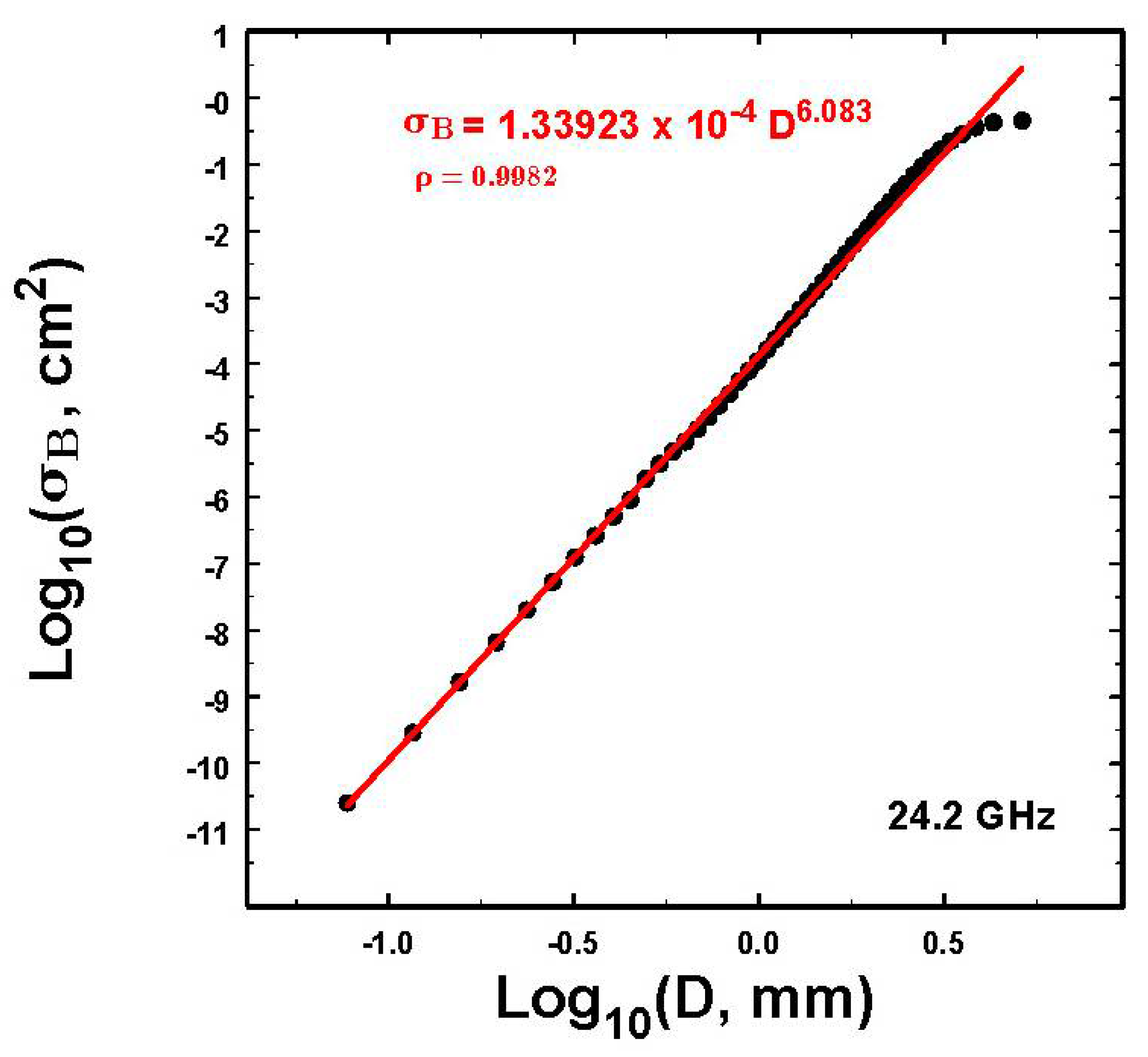
Appendix A.1. Backscatter Cross-Sections Used

On a different topic, some reviewers have questioned the accuracy of the T-matrix backscatter cross-sections calculated in [14]. Figure A1 illustrates that the ratio of the T-matrix backscatter cross-sections to Rayleigh scatters is consistent with that published in the literature for the MRR. The T-matrix values are, therefore, quite acceptable.
Figure A1. The ratio of the T-matrix calculated backscatter cross-sections for spherical raindrops to that expected if the scattering were Rayleigh. The inset corresponds to that reported in the MRR literature showing that the backscatter cross-sections used in this study are in agreement.
Atmosphere 12 00699 g0a1

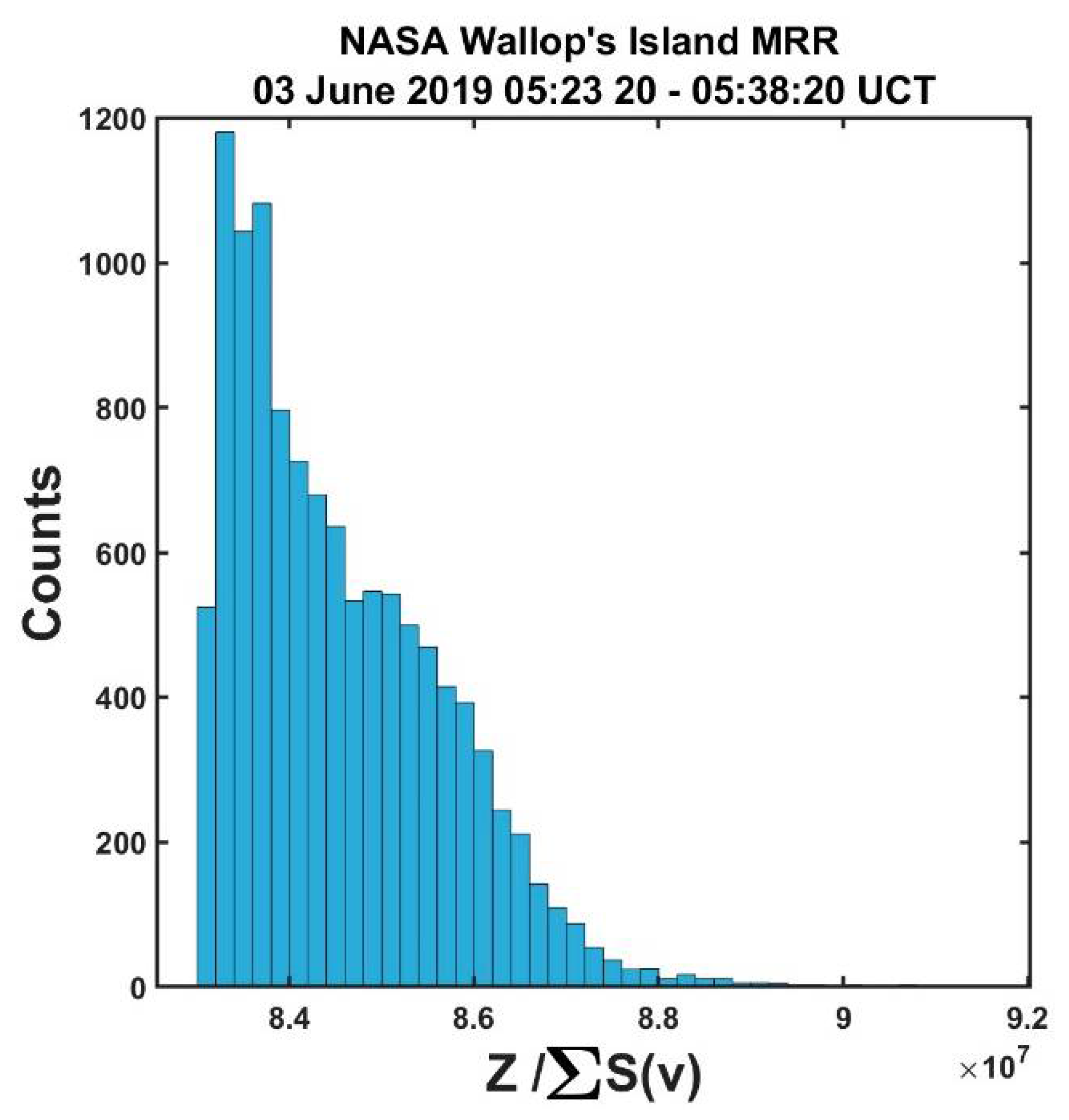
Appendix A.2. Corrections to MRR Z

The Doppler spectra for the MRR radar are the attenuated power spectra. In order to properly apply the technique described in this work, it is necessary to use the effective reflectivity factors that would correspond to these spectra. The MRR provides measurements of the attenuated reflectivity Za and estimates of the equivalent reflectivity factor Ze calculated by using the drop size distributions deduced from the spectra under the assumption that the vertical air velocities were null. As shown in the paper, this is not usually a good assumption that likely contains unaccounted attenuation. A different approach is used here.
Specifically, for the nominal reported wavelength of 1.24 cm for the MRR radar, expression (5) in the paper can be written in terms of logarithms as
Z e ( dB ) = 79.241 ( dB ) + S ( v ) ( dB )
where λ = 1.24 cm, Ze is in mm6 m−3, and η is in m−1, while η is the sum over the Doppler spectrum, η = ∑S(v). A similar expression can be written for Za as well except that it contains the unknown attenuation component, A, namely
Z a ( dB ) = 79.241 ( dB ) + S ( v ) ( dB ) A ( dB ) = [ 79.241 ( dB ) A ( dB ) ] + S ( v ) ( dB )
where A is used as a characteristic measure of the net total attenuation affecting the relation. The expressions equivalent to (A1) and (A2) for the earlier period data are shown in Figure A2.
Figure A2. Linear fits of the logarithms of the MRR-reported equivalent radar reflectivities, Ze, and the attenuated reflectivities vs. the logarithms of the summations over the reported Doppler spectral powers. SE is the standard error of the fits.
Atmosphere 12 00699 g0a2
Clearly, Za is affected by varying amounts of attenuation evident by the spread in the ∑S(v). While some spread may also arise from non-Rayleigh scattering, the largest effects in rain will be likely largely from attenuation.
In contrast, for the later data, the resulting fits are shown in Figure A3.
Figure A3. As in Figure A1, linear fits of the logarithms of the MRR-reported equivalent radar reflectivities, Ze, and the attenuated reflectivities vs. the logarithms of the summations over the reported Doppler spectral powers but for the later period. SE is the standard error of the fits.
Atmosphere 12 00699 g0a3
In this case, Ze will mostly match Za simply by subtraction. This can be determined by looking at the end farthest to the left when attenuation should be at a minimum, so that the shift represents some other change in the system aside from attenuation. However, at larger ∑S(v), some additional adjustment has to be included, as is evident in Figure A3, where the separation between the Za and the Ze lines increase with increasing ∑S(v), likely because of increasing attenuation. Thus, for the later set of data, Ze only had to be mostly adjusted downward to get solutions using (10), as Figure A3 illustrates.
However, attenuation was a more severe problem in the earlier set of data, as shown in Figure A1. While one could try to correct each time period at each altitude for the accumulated attenuation, such a procedure seems unwarranted given the uncertainties in the observations and estimates of the attenuation as well as the unknown error propagation that could occur. For now, instead, we use the difference between the fits to the MRR-reported Za and the Ze as a measure of the characteristic A. This turns out to be equivalent to the shift between the Za and the Ze fits plus the combined standard errors given in Figure A2, which are used to provide a measure of this spread caused by the attenuation. This procedure produces solutions using (10) throughout most of the data field. The final resulting fit for these data is illustrated in Figure A4. It is close to theoretical expectations as given in (A2).
Figure A4. Resulting relation between Ze and ∑S(v) after the adjustments for attenuation to the Ze in Figure A1, as described in the text.
Atmosphere 12 00699 g0a4

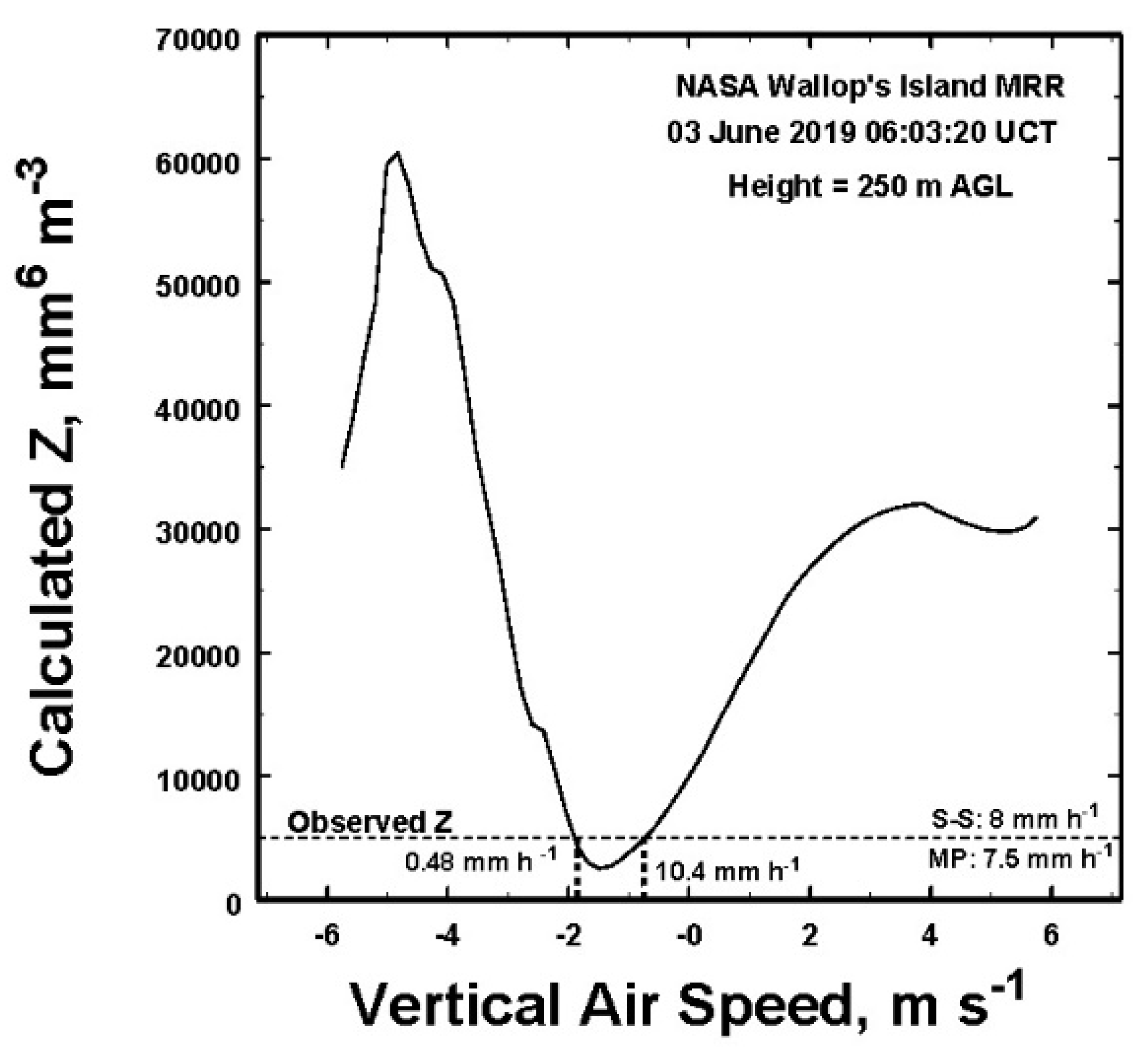
Appendix A.3. Examples of Solution Time–Height Profiles

Figure A5 shows the solution space for (a) the earlier period and (b) the later period. The black areas indicate where there were no solutions because there were no back-scattered powers. Obviously, elsewhere, solutions using (10) were universal in both sets of data after optimizing the MRR data, as discussed in Appendix A.2.
Figure A5. Plots of the solution spaces using (10) for the earlier time period (a) and the later time period (b). Solutions were found throughout except at the locations in black where there were no back-scattered powers.
Atmosphere 12 00699 g0a5

References

  1. Probert-Jones, J.R.; Harper, W.G. Vertical Air Motion in Showers Revealed by Doppler Radar. In Proceedings of the Preprints of Papers; American Meteor Society: Kansas City, MO, USA, 1961; pp. 225–232. [Google Scholar]
  2. Caton, P.G.F. A Study of Raindrop-Size Distribution in the Free Atmosphere. Q. J. R. Meteorol. Soc. 1966, 92, 577–579. [Google Scholar] [CrossRef]
  3. Toit, P.S.D. Doppler Radar Observation of Drop Sizes in Continuous Rain. J. Appl. Meteorol. 1967, 6, 1082–1087. [Google Scholar] [CrossRef] [Green Version]
  4. Spilhaus, A.F. Raindrop Size, Shape and Falling Speed. J. Meteorol. 1948, 5, 108–110. [Google Scholar] [CrossRef] [Green Version]
  5. Gunn, R.; Kinzer, G.D. The Terminal Velocity OffallL for Water Droplets in Stagnant Air. J. Meteorol. 1949, 6, 243–248. [Google Scholar] [CrossRef] [Green Version]
  6. Foote, G.B.; Du Toit, P.S. Terminal Velocity of Raindrops Aloft. J. Appl. Meteorol. 1969, 8, 249–253. [Google Scholar] [CrossRef] [Green Version]
  7. Battan, L.J. Some Observations of Vertical Velocities and Precipitation Sizes in a Thunderstorm. J. Appl. Meteorol. 1964, 3, 415–420. [Google Scholar] [CrossRef] [Green Version]
  8. Rogers, R.R. An Extension of the Z-R Relation for Doppler Radar. In Proceedings of the Preprints of Papers; American Meteor Society: Boulder, CO, USA, 1964; pp. 158–161. [Google Scholar]
  9. Rogers, R.R. Doppler Radar Investigation of Hawaiian Rain1. Tellus 1967, 19, 432–455. [Google Scholar] [CrossRef]
  10. Lhermitte, R.M. Observation of Rain at Vertical Incidence with a 94 GHz Doppler Radar: An Insight on Mie Scattering. Geophys. Res. Lett. 1988, 15, 1125–1128. [Google Scholar] [CrossRef]
  11. Sekhon, R.S.; Srivastava, R.C. Doppler Radar Observations of Drop-Size Distributions in a Thunderstorm. J. Atmos. Sci. 1971, 28, 983–994. [Google Scholar] [CrossRef] [Green Version]
  12. Löffler-Mang, M.; Kunz, M.; Schmid, W. On the Performance of a Low-Cost K-Band Doppler Radar for Quantitative Rain Measurements. J. Atmos. Ocean. Technol. 1999, 16, 379–387. [Google Scholar] [CrossRef]
  13. Jana, S.; Rakshit, G.; Maitra, A. Aliasing Effect Due to Convective Rain in Doppler Spectrum Observed by Micro Rain Radar at a Tropical Location. Adv. Space Res. 2018, 62, 2443–2453. [Google Scholar] [CrossRef]
  14. Jameson, A.R. A Comparison of Microwave Techniques for Measuring Rainfall. J. Appl. Meteorol. 1991, 30, 32–54. [Google Scholar] [CrossRef] [Green Version]
  15. Atlas, D. Advances in Radar Meteorology. In Advances in Geophysics; Elsevier: Amsterdam, The Netherlands, 1964; Volume 10, pp. 317–478. ISBN 978-0-12-018810-9. [Google Scholar]
  16. Marshall, J.S.; Palmer, W.M.K. The Distribution of Raindrops with Size. J. Meteorol. 1948, 5, 165–166. [Google Scholar] [CrossRef]
  17. Jameson, A.R.; Larsen, M.L.; Kostinski, A.B. Disdrometer Network Observations of Finescale Spatial–Temporal Clustering in Rain. J. Atmos. Sci. 2014, 72, 1648–1666. [Google Scholar] [CrossRef] [Green Version]
  18. Jameson, A.R.; Larsen, M.L. The Variability of the Rainfall Rate as a Function of Area. J. Geophys. Res. Atmos. 2016, 121, 746–758. [Google Scholar] [CrossRef] [Green Version]
  19. Beard, K.V.; Jameson, A.R. Raindrop Canting. J. Atmos. Sci. 1983, 40, 448–454. [Google Scholar] [CrossRef] [Green Version]
  20. Williams, C.R. Simultaneous Ambient Air Motion and Raindrop Size Distributions Retrieved from UHF Vertical Incident Profiler Observations: Simultaneous Ambient Air Motion and Raindrop Size Distributions. Radio Sci. 2002, 37, 8-1–8-16. [Google Scholar] [CrossRef] [Green Version]
  21. Schumacher, C.; Stevenson, S.N.; Williams, C.R. Vertical Motions of the Tropical Convective Cloud Spectrum over Darwin, Australia: Vertical Motions of the Tropical Convective Cloud Spectrum. Q. J. R. Meteorol. Soc. 2015, 141, 2277–2288. [Google Scholar] [CrossRef]
  22. Brawn, D.; Upton, G. On the Measurement of Atmospheric Gamma Drop-Size Distributions. Atmos. Sci. Lett. 2008, 9, 245–247. [Google Scholar] [CrossRef]
Figure 1. A plot of the T-matrix computed [14] backscatter cross-sections σB of spherical raindrops of size D (appropriate for vertical pointing observations) corresponding to the Micro-Rain Radar (MRR). The validity of these cross-sections is illustrated in Figure A4 in Appendix A. While there is a slight roll-off at the very largest D, these drops rarely contribute much to most rainfall rates or even Z, so that these deviations are likely usually inconsequential.
Atmosphere 12 00699 g001
Figure 2. The volume flux of raindrops falling at terminal velocity, Vt, as a function of spherical drop size.
Atmosphere 12 00699 g002
Figure 3. Histogram of the ratio of the measured radar reflectivity to the sum of the power densities over the Doppler spectrum showing variable rather than a constant value.
Atmosphere 12 00699 g003
Figure 4. An example of the application of the approach described in the text. The solid line represents the theoretical calculated radar reflectivity (vertical axis) using (10), while the dashed line represents the MRR measured value. There are two solutions for the vertical air velocity, w, one of which is the preferred, as discussed in the text.
Atmosphere 12 00699 g004
Figure 5. A plot of the difference between the measured (Zm) and the calculated Z (Zcalc), illustrating that the likely correct solution (ZSolution) is associated with large values of the total number of drops as appears to always be the case in this study.
Atmosphere 12 00699 g005
Figure 6. The contour plot of the time–height values of the log of the measured rainfall rates, Rm, reported by the MRR processor, computed assuming that there is no vertical air velocity. Note the weak value except near the top of the figure. Times are UCT, and a log scale is used to highlight the weak structure.
Atmosphere 12 00699 g006
Figure 7. The time–height plot of air velocity corrected rainfall rate (Rw) corresponding to Figure 6. Note the dramatic vertical shafts of rain that are now apparent as well as the disappearance of the spurious values at the top compared to the previous figure. Note also the general significant increase in the values of R.
Atmosphere 12 00699 g007
Figure 8. The time–height plot of the relative dispersion = σRw/Rw corresponding to Figure 7. Note that in this instance, throughout most of the domain the relative dispersion is unity or smaller.
Atmosphere 12 00699 g008
Figure 9. (a) The time–height plot of the measured MRR measured radar reflectivity for this time period and (b) the calculated solution values (ZSolution). Note the vertical structure in Z as reflected by the rainfall rates in Figure 7. The added jitter in (b) is due to the quantization of the velocity bins. The black denotes no power observed.
Atmosphere 12 00699 g009
Figure 10. Histograms of the MRR measured (subscript Obs, solid bars) and of the solution (subscript Sol, red empty bars) radar reflectivities in Figure 8 showing the excellent matching, suggesting the general validity of the solutions.
Atmosphere 12 00699 g010
Figure 11. Z–R correlations derived (a) for the rainfall rates adjusted for vertical air speed and (b) those from the MRR processor, as discussed further in the text.
Atmosphere 12 00699 g011
Figure 12. The air vertical velocities, w, derived using the approach described in the text. Note the coherent temporal and spatial structure of the winds with weak updrafts and downdrafts in the center and stronger downdrafts on each side. The velocity magnitudes are also consistent with the observations of others elsewhere, as discussed in the text.
Atmosphere 12 00699 g012
Figure 13. The time–height plots of (a) the observed radar reflectivity Z and (b) ZSol from the solutions for the earlier, more convective time period on this day. Finer structure is apparent in (b), but the values are nearly identical on the whole, as indicated in the next figure. Black denotes no usable power observations after adjustment.
Atmosphere 12 00699 g013
Figure 14. Histograms of the MRR measured (Obs) and solution radar reflectivities in Figure 13 showing the excellent matching suggesting the general validity of the solutions.
Atmosphere 12 00699 g014
Figure 15. Time–height plots of the rainfall rates (a) from the MRR processor (Rraw) and (b) those after accounting for vertical air speed (RSol). Compared to (a), note the significantly larger values throughout (b), which are consistent with the structure of Z in Figure 13. Black denotes no power.
Atmosphere 12 00699 g015
Figure 16. The time–height plot of the relative dispersion = σRw/Rw corresponding to Figure 15b. Note that in contrast to Figure 8 for the later period, in this instance there are many locations where the relative dispersion is 2 or greater.
Atmosphere 12 00699 g016
Figure 17. The air vertical velocities derived using the approach described in the text. Note the coherent but smaller scale temporal and spatial structure of the winds compared to those found in the later time period (Figure 11) likely reflecting the more convective nature of these data. Spectral folding occurred in a few locations leading to the enhanced velocity scale. The large black areas are due to a lack of power, while smaller ones are where no solutions were found without having to further process the data.
Atmosphere 12 00699 g017
Figure 18. ZR correlations derived (a) for the measured rainfall rates (Rm) from the MRR processor and (b) those corrected for vertical air speed (Rw), as discussed further in the text.
Atmosphere 12 00699 g018
Figure 19. Comparisons of the MRR measured (black lines) average one-minute rainfall rates (Rm) at 20 m AGL and of the air velocity adjusted (red lines) rainfall rates (Rw) with the nearby 2DVD estimated rainfall (blue lines), as discussed in greater detail in the text for (a) the more convective time period and (b) for the later time period. Note the poor performance of the measured MRR values in (b).
Atmosphere 12 00699 g019
Publisher’s Note: MDPI stays neutral with regard to jurisdictional claims in published maps and institutional affiliations.

