Comparative Analysis of Three Methods for HYSPLIT Atmospheric Trajectories Clustering

Abstract

Using the Hybrid Single-Particle Lagrangian Integrated Trajectory (HYSPLIT) model to obtain backward trajectories and then conduct clustering analysis is a common method to analyze potential sources and transmission paths of atmospheric particulate pollutants. Taking Qingdao (N36 E120) as an example, the global data assimilation system (GDAS 1°) of days from 2015 to 2018 provided by National Centers for Environmental Prediction (NCEP) is used to process the backward 72 h trajectory data of 3 arrival heights (10 m, 100 m, 500 m) through the HYSPLIT model with a data interval of 6 h (UTC 0:00, 6:00, 12:00, and 18:00 per day). Three common clustering methods of trajectory data, i.e., K-means, Hierarchical clustering (Hier), and Self-organizing maps (SOM), are used to conduct clustering analysis of trajectory data, and the results are compared with those of the HYSPLIT model released by National Oceanic and Atmospheric Administration (NOAA). Principal Component Analysis (PCA) is used to analyze the original trajectory data. The internal evaluation indexes of Davies–Bouldin Index (DBI), Silhouette Coefficient (SC), Calinski Harabasz Index (CH), and I index are used to quantitatively evaluate the three clustering algorithms. The results show that there is little information in the height data, and thus only two-dimensional plane data are used for clustering. From the results of clustering indexes, the clustering results of SOM and K-means are better than the Hier and HYSPLIT model. In addition, it is found that DBI and I index can help to select the number of clusters, of which DBI is preferred for cluster analysis.

1. Introduction

Air pollution is harmful to human health. Every year, many people die prematurely because of air pollution [1]. Air mass trajectories can be used to analyze the transport of air pollutants between regions [2,3,4,5,6]. An important input for air mass trajectory models is meteorological data.

Assuming that air mass movement depends only on wind history, the backward trajectory model of the atmosphere can be established by using vertical profiles of wind vectors in meteorological data. A large amount of backward trajectory data is needed to study the dominant wind direction in a particular region, which requires the trajectory data to be clustered.

In the beginning, data classification is based on the empirical judgment of researchers, which has too many subjective factors [7,8,9]. With the development of computer technology, clustering algorithms emerge in the field of machine learning, which is designed to process data classification without known labels. This coincides with the classification and processing of trajectory data. Some researchers used the clustering algorithm on the trajectory data [9,10]. Trajectory coordinates were used as clustering variables for the first time. Various other clustering algorithms have been used in recent studies. To the authors’ knowledge, there are two main methods of statistical clustering: the hierarchical [11,12,13,14] and the non-hierarchical (e.g., K-means) [12,15,16,17,18,19]. Sirois et al. [15] developed a way to measure the distance between trajectories using mean angles. Wang et al. [11] used the backward trajectory to determine the potential source of PM10 pollution in Xi’an, China. In Wang’s study, Ward’s hierarchical method and mean angles were used to form the trajectory clusters. Li et al. [20] also used mean angles to carry out cluster analysis on the trajectory and found that the seasonal transport pathways of PM2.5 changed significantly. Wang et al. [21] developed a software to identify potential sources from long-term air pollution measurements. Borge et al. [19] used a two-stage cluster analysis (based on the non-hierarchical K-means algorithm) to classify backward trajectories arriving in three different areas in Europe. It was highlighted that when Euclidean distances were used, shorter trajectories were more likely to be assigned to the same cluster, and longer trajectories were more likely to be assigned to different clusters. Therefore, the short trajectories were clustered again. Markou et al. [18] also used a two-step method, but the difference was that he first divided the trajectories into three clusters according to their length and then clustered them separately. Moreover, he used the great circle distance for clustering instead of the Euclidean distance. This approach alleviated the problem that short trajectories were more likely to be clustered together.

However, in recent years, neural networks [12,22,23] and fuzzy c-means [24,25] have been applied. Kassomenos et al. [12] compared the sensitivity of the Self-organizing map (SOM), Hierarchical clustering (Hier), and K-means methods. For different arrival heights, hierarchical clustering showed higher sensitivity, followed by SOM, and K-means was the method least affected by arrival height. Karaca et al. [23] used SOM to conduct clustering analysis on the trajectory data and proposed to use validity index I to select the cluster number. Kong et al. [24] questioned Borge’s [19] argument because, in Markou’s [18] results, there were more clusters in the long-distance trajectory data. At the same time, the Euclidean distance was proposed to replace the Mahalanobis distance, so that the trajectory data could be clustered in one step. The Hybrid Single-Particle Lagrangian Integrated Trajectory (HYSPLIT, release Version 4) model introduced a functional module of cluster analysis. An accurate description of the algorithm can be found in Stunder [26] and Rolph et al. [27]. Su et al. [28] and Bazzano et al. [29] used this method to perform clustering analysis. As for the analysis of the three algorithms, Kassomenos et al. [12] focused on the analysis and comparison of the algorithm results combined with the actual situation of the region. In atmospheric trajectory clustering, the stability and quality of various algorithms need more work and discussion. Based on Kassomenos’s research, this paper compared the calculation process of the three algorithms, evaluated the stability and quality of the three algorithms in the atmospheric trajectory data, and presented some guidance and suggestions for the selection of clustering numbers.

The purpose of the present study was to compare the results of several clustering methods (Hier, K-means, and artificial neural network SOM) and provide reference evidence for future researchers to choose a trajectory clustering analysis method. It is more representative to compare these algorithms which have been used in atmospheric trajectory clustering [12,20,23]. A better clustering algorithm can allow to obtain more stable and accurate results with smaller in-cluster distances and larger distances between clusters.

2. Data and Methods

2.1. Input Data and Model

Three-day backward trajectories arriving in Qingdao (36.0° N, 120.0° E), China, computed at 0, 6, 12, 18 UTC (i.e., 8, 14, 20, 2 (2nd day) local time) for every day during a 4-year period (2015–2018) were used. The four moments every day were selected to increase the number of trajectories. Four years of daily trajectory sets were used as input to the different clustering algorithms at three different arrival heights (10, 100, and 500 m above the ground). These arrival heights were selected by referencing Kassomenos et al. [12] for increasing the datasets, each of which refers specifically to the set of all trajectories reaching each height in each year.

The HYSPLIT model developed with National Oceanic and Atmospheric Administration (NOAA) Air Resources Laboratory (ARL) computed these trajectories and performed the clustering analysis.

The averaged wind speed data was used in the calculation of 72 h backward trajectory data and produced by the National Centers for Environmental Prediction Global Data Assimilation System (GDAS 1°). The vertical transport was modeled using the isobaric option of HYSPLIT. The back trajectories were computed every 6 h at three arrival heights.

2.2. Trajectory Clustering

Clustering means that, according to the similarity principle, data objects with higher similarity can be divided into the same cluster, and data objects with higher heterogeneity can be divided into different clusters. In contrast to classification, clustering is an unsupervised learning process, which means that clustering does not require the training of the model based on the classified data.

In this study, the specific clustering numbers are not fixed; thus, the three clustering algorithms are compared and analyzed under different clustering numbers. The trajectory is defined as the line of 73 backward nodes, and the time interval between adjacent nodes is 1 h. Each trajectory contains 219 values which are the coordinate points of the trajectory. Euclidean distance is chosen in the measurement since it is undoubtedly a very convenient measurement method. Although the Euclidean distance can lead to clustering results in which shorter trajectories are more likely to cluster together, this phenomenon exists in each algorithm and does not affect the conclusion of the study.

2.3. Self-Organizing Maps (SOM)

Self-organizing mapping is a type of self-organizing (competitive) neural network proposed by Kohonen et al. [30]. This clustering algorithm has been used in previous studies due to its characteristic, which is an unsupervised classification model, since the clustering result of trajectory data is also unknown. This algorithm assumes that there is some topological structure or sequence in the input object, which can realize the dimensionality reduction mapping from the input space (i.e., m dimension) to the output plane (i.e., 2 dimensions). The mapping has the property of maintaining topological features, which has a strong theoretical connection with the actual brain processing.

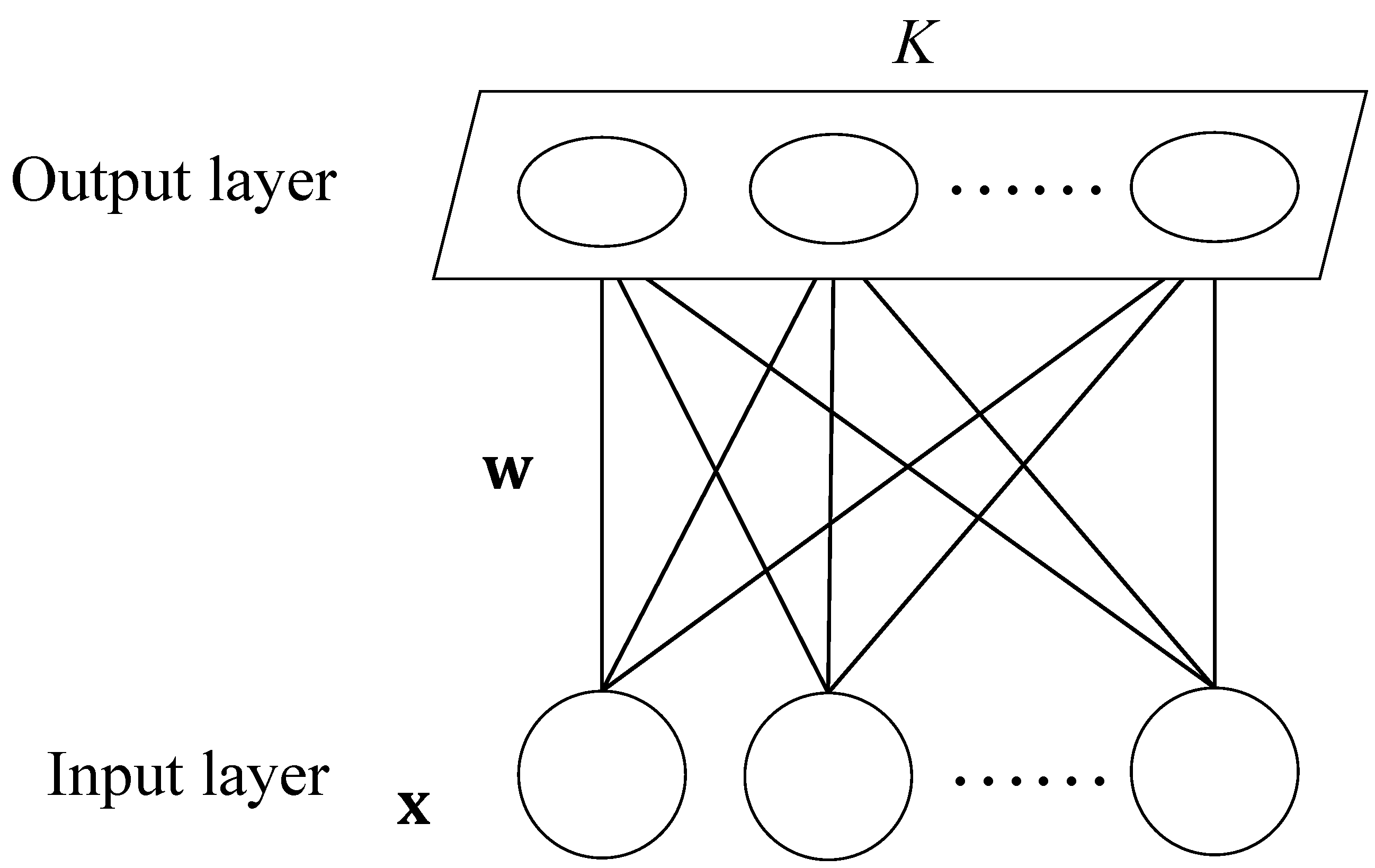
The network is composed of one input layer and one output layer, in which the number of neurons in the input layer is chosen according to the dimensions of the vector in the input network. The input neuron is a one-dimensional matrix that receives the input signals from the network, while the output layer is a two-dimensional node matrix arranged by neurons in a certain way. Neurons in the input layer and neurons in the output layer are connected by weight. When the network receives an external input signal, one of the neurons in the output layer gets excited. In the learning process, the output layer neuron is found with the shortest distance (i.e., excitatory neuron); then, its weight should be updated. At the same time, the weights of the adjacent neurons are updated so that the output node maintains the topological characteristics of the input vector. The algorithm stops when iterations reach the maximum, which is generally 1000. In the clustering analysis, each output neuron corresponds to one cluster. When different signals activate the same excitatory neuron, they belong to the same cluster.

The excitatory neurons are selected according to Equation (1), where x is the input data, $w_j$ is the weight vector, and $d_j\left(x\right)$ is the distance between the input data and the j th output neuron. If $d_j\left(x\right)$ is the smallest value in the $d\left(x\right)$, the jth output neuron is the excitatory neuron. The calculation of the Euclidean distance is similar to Equation (1), thus it is used to compare algorithms.

$$d_j(x)={\displaystyle \sum {(x-w_j)}^2},$$

(1)

Due to the small number of output neurons (the maximum number is 10), only the weights associated with excitatory neurons are updated. The weight updating process is shown in Equation (2), where $\mathsf{\Delta }{w}_j$ is the increment of $w_j$, and $\eta \left(t\right)$ is the learning rate. The value of $\eta \left(t\right)$ drops linearly from 0.5 to 0 over time.

$$\Delta w_j=\eta (t)(x-w_j),$$

(2)

Considered the topological relationship of trajectory data, the (1 × K) output layer structure was selected, where K represents the number of clustering in this study. The SOM structure used is shown in Figure 1. It consists of one input layer and one output layer. The input parameters are values of the trajectory data, and the number of neurons in the output layer depends on the number of clustering. In this study, the number of iterations is 1000.

2.4. Hierarchical Clustering (Hier)

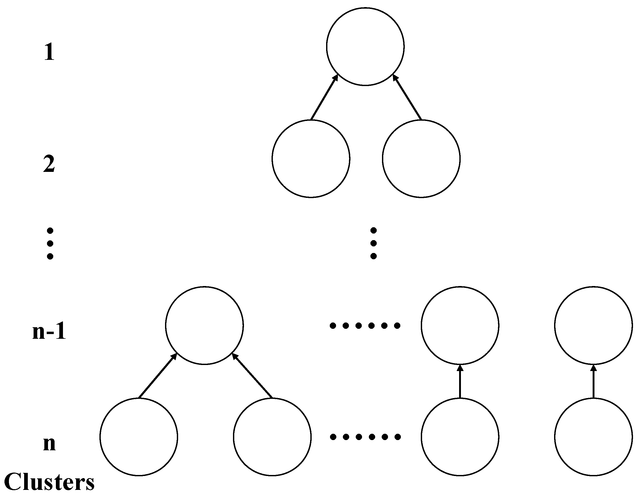
Hier is a type of clustering algorithm, which creates a hierarchical nested clustering tree by calculating the similarity between different kinds of data points. In a cluster tree, the original data points of different clusters are the lowest layer of the tree, and the top layer of the tree is the root node of a cluster. There are two methods to create a cluster tree: bottom-up merging and top-down splitting. By calculating the similarity, the merging algorithm combines the two most similar points into one cluster. The cluster calculates again with other points. This process repeats until all the data is combined into one cluster. The merging algorithm determines the similarity by calculating the distance between clusters. The smaller the distance, the higher the similarity. The two closest data points or clusters are combined to generate a cluster tree.

The algorithm process of hierarchical clustering is shown in Figure 2. The calculation equation for the distance between two clusters is shown in Equation (3), where ${\mu }^{\prime }$ is denoted as the cluster center after merging, ${\mu }_1$,${\mu }_2$ are the cluster centers before merging, $x_1$ is all data in ${\mu }_1$ cluster, $x_2$ is all data in ${\mu }_2$ cluster, $d_{dist}\left(x_1,{\mu }_1\right)$ is the distance of $x_1$ and ${\mu }_1$, $\mathsf{\Delta }D$ is the distance difference before and after merging. If $\mathsf{\Delta }D$ is the minimum between two clusters, the two clusters are merged.

$$\mathsf{\Delta }D={\displaystyle \sum d_{dist}{}^2(x_1,{\mu }^{\prime })}+{\displaystyle \sum d_{dist}{}^2(x_2,{\mu }^{\prime })}-{\displaystyle \sum d_{dist}{}^2(x_1,{\mu }_1)}-{\displaystyle \sum d_{dist}{}^2(x_2,{\mu }_2)},$$

(3)

The HYSPLIT clustering algorithm is also a bottom-up merging algorithm in hierarchical clustering, but different from traditional hierarchical clustering, it uses special data preprocessing methods. The specific algorithm can be found in Stunder [26] and Rolph et al. [27]. In the study, the input parameters are values of the trajectory data. The results are selected by the cluster number.

2.5. K-Means Algorithm

K-means clustering is the most famous partitioning clustering algorithm, which is the most widely used among all clustering algorithms due to its simplicity and efficiency [31]. The idea of the K-means algorithm is to divide a given sample set into K clusters according to the size of the distance between samples. Initially, the centers of K clusters are randomly selected, and all data points are assigned to the nearest center. The distance between the object and the center is calculated using Euclidean distance (there are many options; Euclidean distance is used in this study). By calculating the mean value of the inner points of the cluster, the center of the cluster is recalculated. This process, redistribution of data points and re-establishment of centers, is iterated until the centers of K clusters are fixed.

The result of K-means is very sensitive to the position of the initial center. Arthur’s method is used to select the initial clustering center [32]. The first cluster center is chosen uniformly at random, after which each subsequent cluster center is randomly chosen from the remaining data points. This selection is done with the probability proportional to its distance from the point’s closest existing cluster center. The equation for the probability that each point is selected as the center is shown in Equation (4), where s denotes the number of selected centers, $x_r$ is one of the remaining points, $D\left(x_r\right)$ is the distance from $x_r$ to the point’s closest existing cluster center, and is the probability that $x_r$ is chosen as the center.

$$p_r=D^2(x_r)/{\displaystyle \sum _{i=1}^{n-s}{D}^2(x_i)},$$

(4)

In this paper, the input parameters of K-means are the values of trajectory data. The termination condition of iteration is that no data are allocated to the new cluster or the number of iterations reaches 1000.

2.6. Clustering Metrics

Clustering metrics are also called clustering validity indexes. Clustering validity indexes can evaluate the clustering results and select the number of clustering. It can make the clustering algorithm get better results.

There are two broad categories of clustering performance measures. One is to compare the clustering result with a reference model, which is called the external index. The other category, which looks directly at the clustering results without using any reference model, is called the internal index. In this study, the following four internal cluster validity indices have been used [23,33,34].

Davies–Bouldin Index [35] (DBI): The index is the ratio of the distance within the cluster to the distance between the clusters. When this value is smaller, it means that the distance within the cluster is smaller, and the distance between the clusters is larger. DBI is presented in Equation (5), where K denotes the number of clusters, ${\mu }_k$ means the center of cluster $\mathrm{i}$, $\mathrm{avg}\left(C_i\right)$ is the average distance of cluster $\mathrm{i}$, and $d_{dist}\left({\mu }_i,{\mu }_j\right)$ is the distance of ${\mu }_i$ and ${\mu }_j$.

$$DBI(K)=\frac{1}{K}{\displaystyle \sum _{i=1}^K\underset{j\ne i}{\max }}\left(\frac{avg(C_i)+avg(C_j)}{d_{dist}({\mu }_i,{\mu }_j)}\right),$$

(5)

Index I [33]: The index is defined as Equation (6), where K is the number of clusters, and p is used to compare the results of different cluster configurations. This value is equal to 2, according to Maulik et al. [33]. Here, $E_K$ is the sum of the distances between all data and their cluster center, as shown in Equation (7), where n is the total number of trajectories. Every trajectory $x_j$ belongs to a certain cluster.$u_{kj}$ is a Boolean variable that represents whether the trajectory is of this cluster, belonging to 1, otherwise 0. In addition, $D_K$ is the maximum distance between the cluster center, as shown in Equation (8).

$$I(K)={\left(\frac{1}{K}\times \frac{E_1}{E_K}\times D_K\right)}^p,$$

(6)

$$E_K={\displaystyle \sum _{k=1}^K{\displaystyle \sum _{j=1}^n{u}_{kj}{d}_{dist}(x_j,{\mu }_k)}},$$

(7)

$$D_K=\underset{i,j=1}{\overset{K}{\max }}\left(d_{dist}({\mu }_i,{\mu }_j)\right),$$

(8)

Calinski Harabasz Index (CH) [36]: CH is used to describe the average dispersion degree of clustering results. As the value of CH increases, the distance between clusters increases. The index is defined as Equation (9), where $n_k$ is the number of trajectories of cluster k, and $\mu$ is the center of the entire data set.

$$CH=\left(\frac{{\displaystyle {\sum }_{k=1}^K{n}_k{d}_{dist}{}^2({\mu }_k,\mu )}}{K-1}\right)/\left(\frac{{\displaystyle {\sum }_{k=1}^K{\displaystyle {\sum }_{i=1}^{n_k}{d}_{dist}{}^2(x_i,{\mu }_k)}}}{n-K}\right),$$

(9)

Silhouette Coefficient [37] (SC): The silhouette coefficient indicates the degree to which each data belongs to the cluster. The maximum value is 1, and the minimum value is −1. When SC is greater than 0 and larger, its degree of membership is higher. When SC is less than 0 and closer to −1, it belongs to another cluster.

The index is defined as Equation (10), where $a\left(i\right)$ and $b\left(i\right)$ are the distance to the center of ownership and the distance to the nearest center of non-ownership of the trajectory, respectively.

$$SC(i)=\frac{b(i)-a(i)}{\max \{a(i),b(i)\}},$$

(10)

A low value of SC represents a large in-cluster distance, which indicates that the similarity within the cluster is not high enough. Here, the distance sums the interval of the corresponding values between the two trajectories. As the number of values increases, the distance increases, and the SC value decreases. In this study, the SC value is generally less than 0.5, which means that it is not a good result. The ratio of parts with an SC value greater than 0 to the total data is used to evaluate the clustering results. As shown in Equation (11):

$$S_0=\frac{n_{SC>0}}{n}\times 100\%,$$

(11)

3. Results and Discussion

3.1. The Error Caused by Input Data

Although the preprocessing is different, HYSPLIT is the same algorithm as the Hier compiled by the author. The results of the two algorithms are presented in Section 3. According to the methodology described above, three clustering techniques are applied with different clustering numbers, because the results of the trajectory data are unknown.

The Euclidean distance is calculated as shown in Equation (12), where (E_x1, E_y1) and (E_x2, E_y2) are two coordinate points, and D_Euc is the Euclidean distance between these two points. Directly using the longitude and latitude of each trajectory point as the input data of clustering will lead to wrong clustering results, because longitude and latitude are not plane coordinates.

$$D_{E\mathrm{uc}}=\sqrt{{(E_{x1}-E_{x2})}^2+{(E_{y1}-E_{y2})}^2}$$

(12)

In fact, the distance between the latitude and longitude coordinates should be defined by the great circle distance. As shown in Figure 3, the great circle distance between adjacent longitudes decreases with the increase of latitude. When the coordinates are transformed, the great circle distance from each point on the ellipsoid to Qingdao (36.0° N, 120.0° E) is taken as the Euclidean distance in the new plane coordinate system. Figure 4 shows the different results produced by two different input data.

Converted the coordinate system, the ellipsoid model must be determined. The parameters of the Hier are shown in

Table 1. Coordinate system parameters.

Parameter	Specification
Equatorial radius	6,378,137 m
Oblateness	1/298.257223563
Original point	36.0° N, 120.0° E

Note: the equatorial radius and oblateness are from the WGS 84 ellipsoid.

. A plane coordinate system is established with (36.0° N, 120.0° E) as the origin, the due north axis as the X-axis, and the due east axis as the Y-axis. The Mercator projection is used in the HYSPLIT algorithm. The terrain elevation is very small compared to the value of the earth radius. In this study, the influence of terrain elevation is ignored when the coordinate was converted.

In the coordinate system compiled by the authors, the error increases with the distance between the coordinate point and origin. In contrast, the error in the Mercator projection increases with the distance from the equator. For the coordinate points near Qingdao, the error of the coordinate system from the authors will be smaller.

3.2. Data Dimensionality Reduction

Principal Component Analysis (PCA) is the most commonly used linear dimension reduction method. In the study, the dimension is the number of values in one trajectory. The goal of PCA is mapping high-dimensional data into a low-dimensional space through some kinds of linear projections. The values of trajectory are completely reconstructed in PCA, but retain the characteristics of the original values.

PCA algorithm extracts characteristics from the values of trajectory.

Table 2. The proportion (%) of characteristics represented by all dataset dimensions.

New Values Dimensions	2018			2017			2016			2015
	500 m	100 m	10 m	500 m	100 m	10 m	500 m	100 m	10 m	500 m	100 m	10 m
1	70.7	70.7	70.6	72.6	69.6	67.5	68.4	67	66.9	69.5	68	65.6
2	23.9	23.4	23.2	21.7	23.6	24.9	25.4	25.6	25.4	23.8	24.2	26.3
3	2.5	2.9	3.4	2.9	3.6	4.0	3.0	3.7	4.0	3.3	3.9	4.2
4	1.8	1.8	1.7	1.8	1.9	2.1	2.0	2.3	2.1	2.1	2.4	2.2
5	0.4	0.5	0.5	0.4	0.6	0.7	0.5	0.6	0.7	0.5	0.7	0.8

shows that the two new values through PCA represent 93% of the characteristics contained in the old values. Furthermore, the similarity of clustering is more than 99% between using all values of trajectories and the plane coordinate values of trajectories. This phenomenon which is due to the information carried by the height data has been reflected in the plane coordinates. Since the selected trajectories are time series of the same length, the horizontal distance of the air mass will change correspondingly if the air mass has a great change in height within the same time.

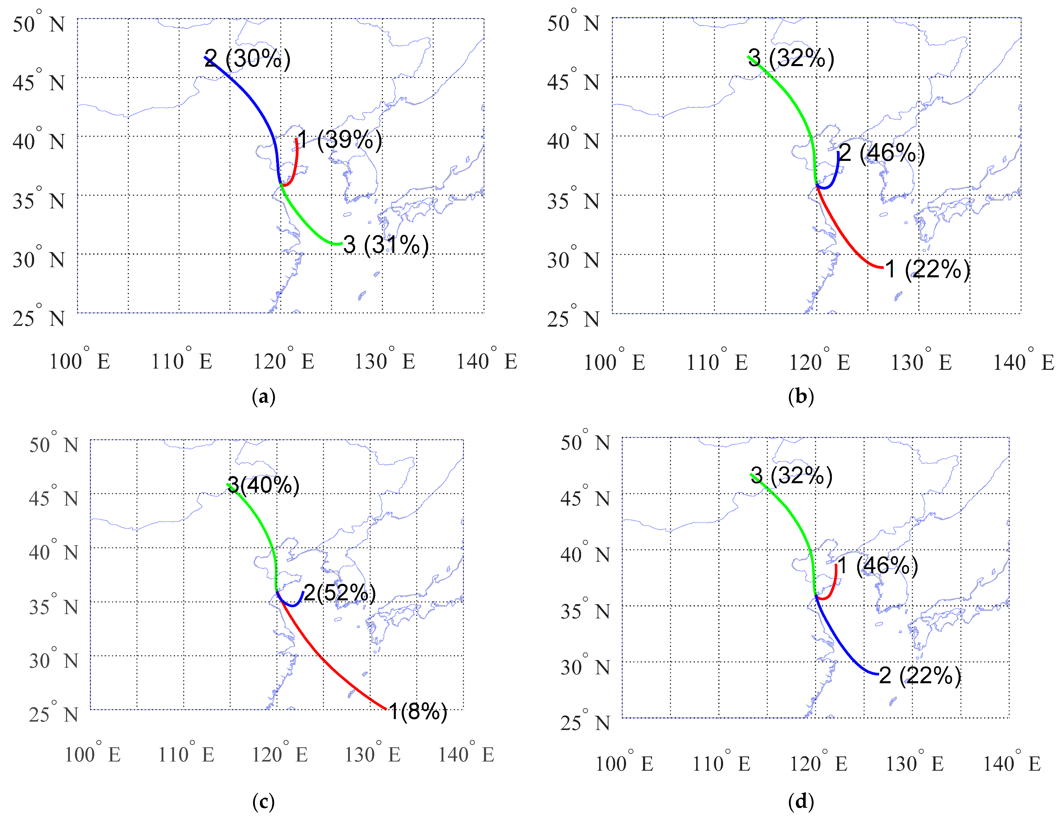
Figure 5 shows a clustering result case of the three algorithms. From this data set of typical results, it can be seen that the results of K-means and SOM are very similar, while the results of HYSPLIT and Hier, which belong to the same algorithm, are not similar. In the following, further analyses are conducted on this situation.

3.3. The Similarity of Algorithms

The similarity between two algorithms S_A is calculated with Equation (13), where $n_i{}^{\prime }$is denoted as the number of the same trajectories in the corresponding clusters between two algorithms.

$$S_A=\frac{{\displaystyle \sum _{i=1}^K{n}_i{}^{\prime }}}{n}\times 100\%$$

(13)

When the similarity between two algorithms is very poor, the search of the corresponding clusters between algorithms needs a subjective judgment according to the direction and length of these cluster centers. Therefore, the more similar the results are, the more accurate the calculation is.

The similarity of clustering result of K-means and SOM algorithm is calculated, and the results from both are highly similar. However, the similarity calculation results of HYSPLIT and Hier show different performances in different data sets. This phenomenon arouses attention and is analyzed.

3.3.1. K-Means and SOM (1 × K)

Similarity analysis shows that the results of SOM (1 × K) and K-means are very similar. Taking the value of K-means as the reference, the similarity results of SOM are shown in

Table 3. Similarity (%) of clustering results between K-mean and SOM.

Similarity(%) Clusters	2018			2017			2016			2015
	500 m	100 m	10 m	500 m	100 m	10 m	500 m	100 m	10 m	500 m	100 m	10 m
2	99.8	99.9	100	100	99.9	99.0	100	100	99.9	100	100	99.9
3	100	99.9	96.0	98.4	99.9	86.6	68.0	99.7	99.7	99.2	99.9	99.7
4	99.5	99.0	99.8	99.8	99.9	99.9	99.3	58.3	99.7	98.2	70.9	89.2
5	99.7	98.7	99.7	99.4	95.7	98.4	99.4	99.2	69.7	99.9	99.7	99.8
6	99.7	99.6	99.4	99.2	63.6	82.3	99.6	99.3	88.2	62.2	64.4	98.3
7	98.6	99.9	99.9	99.5	60.4	69.8	70.1	89.7	99.0	62.7	98.9	82.8
8	92.1	99.3	70.1	75.5	99.6	99.5	99.4	77.2	79.0	98.9	84.2	99.4
9	72.6	76.1	98.9	68.4	66.7	89.0	72.8	67.5	87.6	98.6	89.0	67.4

.

The results show that the two algorithms maintain a high degree of similarity in most cases. Clustering results below 85% similarity are called bad points. Since the result of similarity does not decrease with the increase of cluster number, but suddenly decreases at one cluster number, and then suddenly increases at another cluster, such a bad point is called as “collapse point”. In the SOM (1×n) model, both the first and last neurons have only one neighboring neuron, which may lead to differences with K-means in some cases.

Multiple candidate clustering numbers are selected, and both SOM and K-means clustering algorithms are applied to each candidate clustering number. The result similarity of the two algorithms is calculated. As a rule of thumb, the threshold for similarity is about 85%. If more than one candidate cluster number reaches the threshold value, the multiple results are considered to be reliable. Then, the researcher needs to make a choice.

3.3.2. HYSPLIT and Hier

HYSPLIT and Hier follow the same clustering algorithm. Different projection methods lead to different results in the two algorithms. The similarity between the two algorithms is analyzed in all the data sets. The results are shown in

Table 4. Similarity (%) of clustering results between HYSPLIT and Hier.

Similarity(%) Clusters	2018			2017			2016			2015
	500 m	100 m	10 m	500 m	100 m	10 m	500 m	100 m	10 m	500 m	100 m	10 m
2	93.4	89.8	62.5	99.5	73.9	100	99.9	100	100	92.2	74.9	97.7
3	76.9	33.8	67.9	98.4	72.9	100	96.7	85.9	100	88.2	77.9	61.5
4	53.9	65.3	65.1	69.5	72.9	100	95.2	77	98.9	61.4	61.6	84.6
5	75.8	51.4	69.3	84.5	58.4	100	94.3	61.6	98.4	69.7	87.5	78.7

.

The PCA algorithm can restructure the characteristics using fewer dimensions. Different dimensions used in Hier will cause different results. When the distance between several clusters is close, the differences in preprocessing will cause two different clusters to merge.

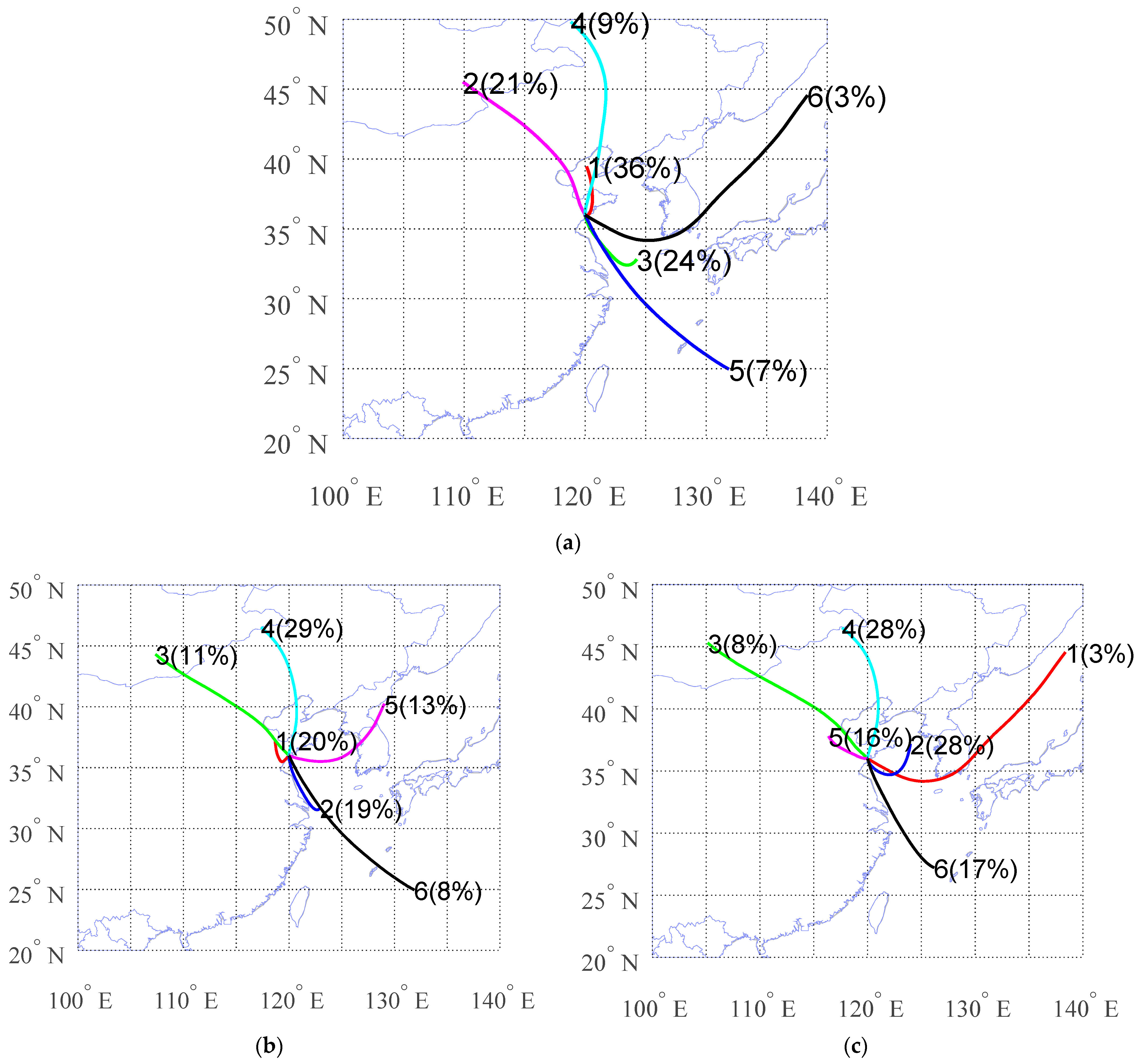
Figure 6a,b shows the clustering results for HYSPLIT and Hier. When the cluster number is 6, the two results differ greatly, and only the results of one cluster are consistent. Figure 6c is the result of clustering after a PCA algorithm preprocessed the data, and all trajectory values kept 99.9% characteristics. After 0.1% characteristics loss, the results change significantly, indicating the instability of Hier’s results.

3.4. Clustering Metrics

3.4.1. The Selection of Cluster Number

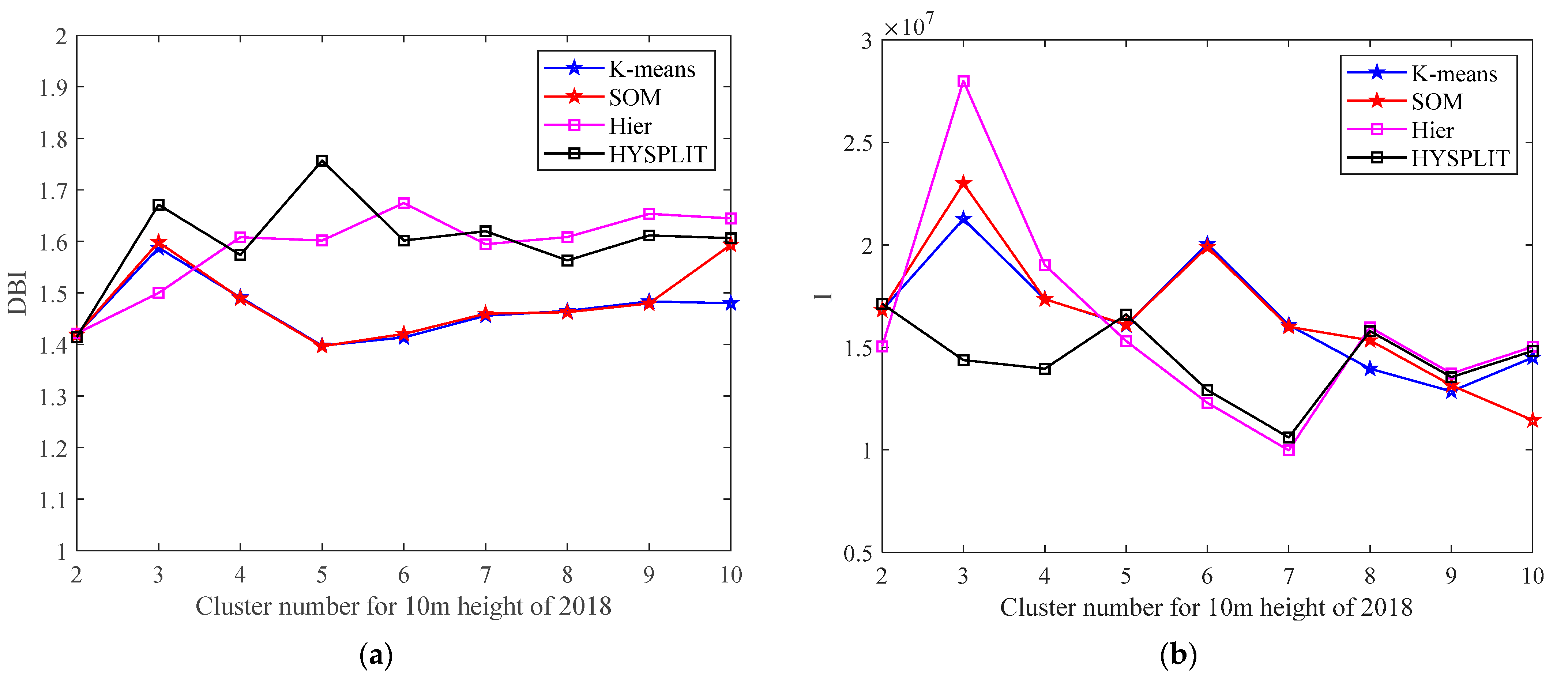
Four kinds of clustering indexes were used to evaluate different clustering numbers. It was found that CH decreased with the increase of clustering number, and no maximum point appeared, which could be used as the basis for the selection of clustering numbers. The results are similar to Karaca’s results [23]. However, DBI and I both generate extreme points, which can be used to select the clustering number. Figure 7 shows the results of 10-m arrival height of 2018 data set.

As can be seen in Figure 7a, DBI maintains a relatively stable situation with low values in some clusters. The low value can be used as a candidate for clustering numbers. In Figure 7b, the values of I grow to a certain point, and then, they start to decline. The maximum point can be used as the candidate point of the clustering number. Due to the low complexity of the wind field variation of the selected location, it can be seen that the clustering number corresponding to the candidate points is small.

3.4.2. Comparison of Clustering Algorithms

The clustering results of the three algorithms are evaluated by four clustering indexes. With the exception of I index, the results of other indexes at different arrival heights are similar.

Table 5. The results of three clustering indexes (DBI, CH, and S₀).

Index	DBI				CH				S0
Clusters	K-Means	SOM	Hier	HYSPLIT	K-Means	SOM	Hier	HYSPLIT	K-Means	SOM	Hier	HYSPLIT
2	1.34	1.34	1.38	1.38	1315	1315	1155	1199	0.99	0.99	0.97	0.95
3	1.60	1.67	1.62	1.64	1048	1016	918	922	0.96	0.89	0.92	0.91
4	1.54	1.57	1.65	1.69	988	975	846	836	0.97	0.97	0.87	0.89
5	1.49	1.50	1.60	1.65	948	943	799	789	0.97	0.97	0.87	0.86
6	1.51	1.52	1.64	1.66	905	898	767	731	0.96	0.96	0.84	0.87
7	1.53	1.56	1.67	1.70	869	861	740	707	0.96	0.95	0.84	0.86
8	1.53	1.54	1.69	1.71	834	828	712	681	0.96	0.95	0.84	0.84
9	1.55	1.58	1.71	1.75	796	793	681	661	0.96	0.96	0.84	0.83

Note: These bold numbers are the best result of each cluster number.

shows the mean values of clustering results of DBI, CH, and S₀ in all data sets.

As can be seen from Table 5, K-means shows the lowest values of DBI, which indicates that the in-cluster distance of K-means clustering result is the shortest. SOM shows the second lowest values of DBI, while Hier and HYSPLIT show poor values. The results of CH are similar to those of DBI, and K-means still shows the best results. CH values of SOM are very close to those of K-means. These results indicate that K-means clustering results have the largest distance between clusters, followed by SOM. When the SC is not performing well, but it can still be used as a reference, S₀ is used. As can be seen from the results of S₀, 10% or more results for HYSPLIT and Hier are incorrectly clustered. The results of incorrect clustering are closer to the center of the other cluster.

In the index of I, these 12 data sets are divided into three groups according to arrival height.

Table 6. The results of I index at the different arrival heights.

Values (×107)	10 m				100 m				500 m
Clusters	K-Means	SOM	Hier	HYSPLIT	K-Means	SOM	Hier	HYSPLIT	K-Means	SOM	Hier	HYSPLIT
2	1.39	1.39	1.28	1.32	2.45	2.44	2.21	2.37	5.46	5.46	5.20	5.07
3	1.54	1.63	1.62	1.22	2.74	2.85	2.90	2.25	4.92	4.71	4.33	4.46
4	1.45	1.45	1.32	1.21	2.29	2.35	2.27	2.42	4.65	4.82	4.55	4.24
5	1.20	1.23	1.04	1.08	1.97	1.94	1.85	1.87	4.26	4.15	4.35	4.09
6	1.23	1.29	1.01	1.03	1.94	1.93	1.58	1.57	3.66	3.63	3.56	3.82
7	1.11	1.07	0.90	0.87	1.67	1.67	1.42	1.30	3.20	3.11	3.01	3.16
8	1.00	1.01	1.02	1.00	1.49	1.51	1.26	1.13	2.82	2.86	2.61	2.78
9	0.93	0.88	0.90	0.88	1.58	1.27	1.22	1.13	2.74	2.63	2.28	2.38

shows the I values of the clustering results at different arrival heights. As the height increases, the value of I gradually increases. This result means that the greater the height is, the farther the distance between clusters is. This phenomenon is caused by the increase in the number of long-distance trajectories as the arrival height increases. The results are similar to those of Markou et al. [18]. In values of I, K-means and SOM perform better than HYSPLIT and Hier. This result indicates that K-means and SOM have the largest distance between clusters. The value of DBI distinguishes the three algorithms more clearly than the value of I. When selecting cluster numbers, DBI is preferred.

4. Conclusions and Future Work

In this paper, the stability and similarity of clustering algorithms (K-means, SOM, and Hier) are compared and analyzed for backward trajectory data of air mass, and 12 data sets are used to ensure the universality of the results. According to the analysis results, the following conclusions can be drawn:

Latitude and longitude coordinates cannot be directly used for clustering analysis. As latitude increases, the great circle distance between adjacent longitudes becomes shorter. Since the Euclidean distance is used as the distance method for clustering, the longitude and latitude coordinates have been converted into plane coordinates for clustering analysis.

The PCA analysis found that the height value carried little information; thus, plane coordinates can be used for cluster analysis. Results from the HYSPLIT and Hier methods are very sensitive to the input data, while SOM and K are not.

SOM (1 × K) and K-means show a high degree of similarity. Both methods should be used for cluster analysis simultaneously to identify the “collapse point”. In the SOM (1 × K) model, both the first and last neurons have only one neighboring neuron, which may lead to differences with K-means in some cases.

HYSPLIT and Hier show a low degree of similarity. The difference of projection methods in the two algorithms leads to different results. Hier uses the projection method with less error.

By analyzing and comparing the results of the three algorithms, the result of SOM (1 × K) and K-means algorithms are stable, and the clustering effect is better. DBI and I index can select the number of clusters, of which DBI is preferred for cluster analysis.

In this work, it is found that K-means and SOM clustering algorithms have a high similarity in trajectory clustering. In future work, we will change the weight update function of the SOM and the arrangement of the output neurons to study the change rule of the results. Atmospheric trajectory models and their clustering results can also play an important role in studying air pollution in China.