Abstract
Reducing PM2.5 and ozone concentrations is important to protect human health and the environment. Chemical transport models, such as the Community Multiscale Air Quality (CMAQ) model, are valuable tools for exploring policy options for improving air quality but are computationally expensive. Here, we statistically fit an efficient polynomial function in a response surface model (pf-RSM) to CMAQ simulations over the eastern U.S. for January and July 2016. The pf-RSM predictions were evaluated using out-of-sample CMAQ simulations and used to examine the nonlinear response of air quality to emission changes. Predictions of the pf-RSM are in good agreement with the out-of-sample CMAQ simulations, with some exceptions for cases with anthropogenic emission reductions approaching 100%. NOx emission reductions were more effective for reducing PM2.5 and ozone concentrations than SO2, NH3, or traditional VOC emission reductions. NH3 emission reductions effectively reduced nitrate concentrations in January but increased secondary organic aerosol (SOA) concentrations in July. More work is needed on SOA formation under conditions of low NH3 emissions to verify the responses of SOA to NH3 emission changes predicted here. Overall, the pf-RSM performs well in the eastern U.S., but next-generation RSMs based on deep learning may be needed to meet the computational requirements of typical regulatory applications.
1. Introduction
PM2.5 and ozone air pollution lead to harmful effects on human health and the environment [1,2]. Air quality management plans are developed to reduce these criteria pollutant concentrations to meet National Ambient Air Quality Standards (NAAQS) in the U.S. [3,4,5]. Air quality modeling with comprehensive chemical transport models (CTMs) contributes key information to air quality planning by providing concentration predictions for baseline and policy-relevant emission-control conditions [6].
Air quality modeling is important for effective air quality management because the response of PM2.5 and ozone to precursor emission changes is nonlinear and depends on hundreds of chemical reactions. For instance, ozone concentrations decrease in response to NOx emission reductions when NOx is the limiting precursor for oxidant formation but increase under NOx-saturated conditions, where NOx inhibits oxidant production [7]. PM2.5 nitrate can also increase or decrease in response to NOx emission reductions depending on oxidant levels and other factors, such as aerosol pH, temperature, and relative humidity [8,9,10,11,12]. Previous studies have individually reported seasonal variations in the nonlinear response of ozone and PM2.5 to NOx emission reductions in the U.S. for retrospective periods [13,14]. However, information is limited on the seasonal variation in the simultaneous response in ozone and PM2.5 and its components for multiple precursors under recent conditions in the U.S. Consideration of relatively recent conditions is important because NOx emissions declined by 57% and SO2 emissions by 85% between 2000 and 2017 (https://gispub.epa.gov/neireport/2017/, accessed on 11 August 2021).
A challenge in using CTMs to explore hypothetical policy options is computational expense. The runtime for CTM simulations (days to weeks) typically prevents direct modeling of the dozens to hundreds of possible emission scenarios that may be of interest to policymakers [15,16,17]. As a result, researchers have developed computationally efficient approaches that approximate CTM capabilities [18,19,20,21,22,23,24,25,26,27]. Of these approaches, response surface models (RSMs) are unique in their ability to simulate the nonlinear response of ozone and PM2.5 over wide ranges of precursor emission changes. RSMs are developed by statistically modeling the results of multiple CTM simulations with a set of explanatory variables based on the emission inputs for each simulation compared to a baseline simulation. After fitting, RSMs can provide predictions of the air quality response to emission changes in near real-time. RSMs have been developed to provide the air quality response to emission changes rather than changes in other variables (e.g., meteorology) because pollutant emissions are the key modifiable factors in air quality management applications.
Early-generation RSMs required large numbers of CTM simulations to produce a statistical fit to capture the complex pollutant responses simulated by CTMs [21,23,28,29]. To reduce the number of simulations for cases with multiple regions and emission control factors, the extended RSM (ERSM) technique was developed [20,24]. Next, using prior knowledge from ERSM results, a polynomial function-RSM (pf-RSM) approach was developed that further reduced the required number of CTM simulations by using polynomial functions to capture the nonlinear response of PM2.5 and ozone to emission changes [19]. Recently, the DeepRSM method [22] has been developed to efficiently calculate the polynomial function coefficients using a convolutional neural network trained with chemical indicators [30]. Much of the development of RSM technology has happened through the ABaCAS (Air Benefit and Cost and Attainment Assessment System, http://www.abacas-dss.com, accessed on 11 August 2021) project, and applications of recent RSMs have been limited to regions in Asia. The performance and applicability of recent RSM methods for the U.S. and other regions needs to be established for these approaches to gain broader use.
In this study, we fit a one-region pf-RSM [19] to CTM simulations over the eastern U.S. for January and July of 2016. We characterize the performance of the pf-RSM using 30 out-of-sample (OOS) CTM simulations. We also provide insights on the nonlinear response of air pollution in the eastern U.S. to anthropogenic emission reductions in winter and summer. We focus here on the response of maximum daily 8 h average (MDA8) of ozone, PM2.5, nitrate, sulfate, and organic matter (OM) concentrations to emission changes of NOx, SO2, NH3, and traditional volatile organic compounds (VOCs). The pf-RSM also simulates the response of PM2.5 concentrations to primary PM2.5 emissions and is available for download.
2. Methods
2.1. Base-Case CTM Simulation
CTM simulations were performed for January and July 2016 with version 5.3.1 of the Community Multiscale Air Quality (CMAQ; https://zenodo.org/record/3585898#.YRXGeEARWUk, accessed on 11 August 2021) model on a domain covering the eastern U.S. with 12 km grid spacing and 35 vertical layers. January and July were selected to be representative of winter and summer conditions, respectively. Gas-phase chemistry was parameterized according to the Carbon Bond 2006 mechanism (CB6r3) [31], the deposition was modeled with the M3DRY parameterization, and aerosol processes were parameterized with the AERO7 module using the non-volatile treatment for primary organic aerosol [32,33]. Chemical boundary conditions were developed from a CMAQ simulation on a larger domain that used boundary conditions from a hemispheric CMAQ simulation [34]. The starting point for the modeled anthropogenic emissions was version 2 of the 2014 National Emissions Inventory (NEI); however, many inventory sectors were updated to represent the year 2016 through the incorporation of 2016-specific state and local data along with nationally-applied adjustment methods [35]. Emissions of anthropogenic precursors for secondary organic aerosol (SOA) [36] were not added to the simulation beyond what was captured in the NEI. Therefore, VOC impacts discussed below are due to traditional VOCs alone. Emissions of biogenic compounds were modeled with the Biogenic Emission Inventory System (BEIS) [37], and emissions of sea-spray aerosol [38] were simulated online within CMAQ using 2016 meteorology. Meteorological fields were developed from a simulation with version 3.8 of the Weather Research and Forecasting model as described elsewhere [39].
Model performance for the base-case CTM simulation was evaluated by comparison with available monitoring data for PM2.5, PM2.5 components, and MDA8 ozone (Supplementary Text S1, Supplementary Table S1) (Supplementary Materials, Tables S1—S4). The model performance statistics are generally within ranges reported in previous applications [40,41] and support the modeling here. However, overpredictions of PM2.5 organic carbon concentrations were evident in January, possibly due to issues with emissions or meteorology as well as gas-particle partitioning of primary organic aerosol. The performance results in Supplementary Table S1 should therefore be considered in interpreting the RSM predictions. Model performance results here are qualitatively consistent with Appel et al. [42], although statistics are calculated for different periods and are not directly comparable across studies.
2.2. Sensitivity CTM Simulations and pf-RSM Development
In addition to the base-case simulation, 22 simulations were conducted for model fitting with domain-wide changes in U.S. anthropogenic emissions of NOx, SO2, VOC, NH3, and primary PM2.5 (see Supplementary Table S3). For 19 of these simulations, emission changes were specified based on Hammersley sampling [43] of emission control ratios between 0 and 1.2 (base case = 1.0). Additionally, one simulation was conducted with 100% reductions in U.S. anthropogenic emissions of NOx, SO2, NH3, and VOCs, and two simulations were conducted with 50% and 100% reductions in primary PM2.5 emissions. Emission-perturbation simulations were implemented in CMAQ using the Detailed Emissions Scaling, Isolation, and Diagnostic (DESID) module [44]. Version 2.5 of the RSM-VAT software was used to implement the Hammersley sampling and generate the emission-control interface files for DESID.
Polynomial functions were fit in each grid cell to provide the nonlinear response of monthly average PM2.5, PM2.5 components, and MDA8 ozone to changes in NOx, SO2, VOC, NH3, and primary PM2.5 emissions across the domain. The following optimized polynomial functions developed in the previous work [19,45] were fit using results of the emission reduction simulations in Supplementary Table S3:
where ΔPM2.5,spc refers to the change from the base case in the concentration of PM2.5, PM2.5 nitrate, PM2.5 sulfate, or PM2.5 organic matter; ΔE refers to the ratio of the difference in emissions between the base and emission perturbation cases to the base emissions (i.e., ΔEi = (Ei − EBase)/EBase); and X1–12 and Y1–7 are the polynomial coefficients determined by least-squares error fitting.
ΔPM2.5,spc = X1 ΔENOX + X2 ΔESO2 + X3 ΔENH3 + X4 ΔEVOC + X5 ΔENOX2 + X6 ΔESO22 + X7 ΔENH32 + X8 ΔENOX ΔEVOC + X9 ΔENOX3 + X10 ΔENOX2 ΔEVOC + X11 ΔENOX2 ΔESO2 + X12 ΔENOX2 ΔENH3
ΔMDA8 O3 = Y1 ΔENOX + Y2 ΔESO2 + Y3 ΔENH3 + Y4 ΔEVOC + Y5 ΔENOX2 + Y6 ΔENOX ΔENH3 + Y7 ΔENOX2 ΔENH3
The pf-RSM was evaluated by comparison with 30 OOS CMAQ simulations that were not used in model fitting (Table S4). The OOS simulations included 10 simulations based on Hammersley sampling and 20 simulations corresponding to 20%, 40%, 60%, 80%, and 100% reductions in U.S. anthropogenic NOx, SO2, NH3, and VOC emissions.
The strength of the RSM is the ability to conduct interactive exploratory analyses on air quality impacts for an unconstrainted number of emission cases using the RSM-VAT software. Below, we focus on comparisons of pf-RSM and CMAQ OOS predictions to demonstrate the performance of the pf-RSM. We also use the OOS simulations to illustrate features of the nonlinear response of ozone and PM2.5 and its components in the eastern U.S. in winter and summer. The RSM-VAT software is available with cases preloaded for exploration of additional scenarios.
3. Results
Predictions of the pf-RSM are compared with CMAQ results for the 30 OOS runs in this section. The comparisons illustrate the performance of the pf-RSM as well as the nonlinear response of PM2.5 and MDA8 ozone to reductions in U.S. anthropogenic emissions. Average monitored concentrations of PM2.5, PM2.5 components, and MDA8 ozone in the region are provided in Supplementary Table S1 and have been discussed in previous studies [14].
3.1. January
The air quality response to emission changes predicted by the pf-RSM and CMAQ are compared for the 30 OOS cases for five species in Figure 1. Overall, there is an excellent correlation and slight bias between the pf-RSM and CMAQ results. However, some distinct features are evident in the scatterplots due to the specific conditions of the individual OOS simulations. For instance, most points in the MDA8 ozone panel are close to the one-to-one line, but a cluster points above the line indicates some overpredictions by the pf-RSM. These points are associated with the case of 100% NOx emission reductions (see Supplementary Figure S1 for scatterplots faceted by OOS case) (Supplementary Materials, Figures S1–S10). Challenges in simulating pollutant response for cases with extreme emission reductions have been reported in the past and suggest a need for including additional CTM simulations in pf-RSM fitting for applications where deep emission reductions may be relevant [19].
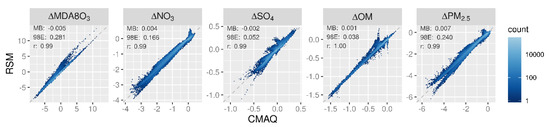
Figure 1.
Comparison of changes in mean January concentrations predicted by the pf-RSM and 30 OOS CMAQ simulations. Units: ppb for MDA8 ozone and μg m−3 for PM2.5 and its components.
pf-RSM predictions of the nitrate response to emission changes also agree well with the OOS CMAQ results, despite some overpredictions of nitrate concentration increases (i.e., disbenefits). These overestimates are associated with cases of SO2 emission reductions, where disbenefits are overpredicted by up to ~0.4 μg m−3 for the case of 100% reduction in anthropogenic SO2 emissions (Supplementary Figure S2). For pf-RSM predictions of the sulfate response, the largest deviations from the one-to-one line in Figure 1 are associated with OOS Run 4 and 5 based on Hammersley sampling of emissions (Supplementary Figure S3). These runs included deep reductions in NOx, VOC, NH3, and SO2 emissions (Supplementary Table S4).
For the OM concentration response, there is good agreement between the pf-RSM and CMAQ predictions in general. However, the pf-RSM predicts some disbenefits for the 100% NOx emission reduction case (Supplementary Figure S4) that were not predicted by CMAQ. For the total PM2.5 concentration response, the scatterplot has a forked shape for concentration decreases larger than 4 μg m−3. This pattern results from the combination of underpredictions in response to the pf-RSM in the 100% NH3 emission reduction case and overpredictions in a case with large NOx reductions (i.e., Run 5 with 97% NOx, 90% SO2, 24% NH3, and 81% VOC emission reductions) (Supplementary Figure S5). This behavior further demonstrates that deviations of the pf-RSM from CMAQ may be relatively large in cases with large emission reductions, and model fitting could be improved by including additional simulations for marginal emission cases. Since emission reductions approaching 100% are uncommon in typical regulatory applications, pf-RSM performance issues for these marginal cases may be of limited concern in many applications.
In Figure 2, the spatial patterns of concentration responses in January 2016 are compared for CMAQ and the pf-RSM for MDA8 ozone, nitrate, sulfate, and OM for 60% reductions in NH3, NOx, SO2, and VOC emissions. The response patterns for the pf-RSM and CMAQ are in good agreement in all cases. NOx emission reductions in January lead to increases in MDA8 ozone over much of the domain (Figure 2a), especially in northern and urban areas (e.g., the mean/max concentration increase above 37° N is 0.8/7.1 ppb for CMAQ). The ozone disbenefits for NOx emission reductions are consistent with oxidant-limited conditions in NOx-rich areas in winter [14,46,47]. By contrast, MDA8 ozone concentrations decrease in response to NOx emission reductions along the Gulf Coast (except Houston) and over Florida, likely due to the lower NOx emissions and inflow of marine air. For VOC, the 60% emission reductions reduce MDA8 ozone concentrations broadly over the eastern U.S. (CMAQ mean reduction: 1.1 ppb).
Figure 2.
Comparison of the change in average concentration in January 2016 for the pf-RSM and CMAQ for a 60% reduction in anthropogenic emissions of NH3, NOx, SO2, and VOC: (a) MDA8 ozone, (b) PM2.5 nitrate, (c) PM2.5 sulfate, and (d) PM2.5 OM. Units: ppb for MDA8 ozone and μg m−3 for PM2.5 components. Statistics for pf-RSM and CMAQ comparison: MB: mean bias; 98E: 98th percentile of error; r: Pearson correlation coefficient.
The 60% reductions in NH3 and NOx emissions reduce nitrate concentrations in the northern part of the domain and demonstrate the sensitivity of nitrate to both precursors there (Figure 2b). NH3 emission reductions in areas of elevated NH3 concentration [48] can reduce nitrate concentrations by increasing particle acidity (due to removal of the key atmospheric base, NH3) and thereby reducing the fraction of total nitrate in the particle phase [9,49,50]. NOx emission reductions reduce nitrate through direct removal of the nitrate precursor, which outweighs the effect of increased NOx-to-nitrate conversion efficiency from increased ozone/oxidant concentrations. For reducing nitrate in January, NH3 emission reductions (mean nitrate reduction: 0.62 μg m−3) are more effective than NOx emission reductions (mean nitrate reduction: 0.46 μg m−3). SO2 and VOC emission reductions have relatively small influence on nitrate, with some nitrate disbenefits for SO2 reductions in the northern part of the domain (likely due to the influence of reduced acidity from lower sulfate on partitioning of total nitrate to the particle phase).
The 60% reductions in NH3 emissions lead to small decreases in sulfate concentrations in the northern part of the domain (Figure 2c). Since sulfate is essentially nonvolatile under atmospheric conditions, NH3 levels do not affect gas-particle partitioning of sulfate as they do for semi-volatile nitrate. However, in-cloud sulfate production is sensitive to cloud pH, and the reductions in NH3 concentrations could reduce cloud pH and thereby lower the rate of S(IV) to S(VI) conversion (e.g., due to ozone pathways, [51]). Shah et al. [52] reported that in-cloud oxidation was responsible for about 65% of the conversion of SO2 to sulfate in the eastern U.S. in winter 2015. NOx emission reductions lead to increases in sulfate in the northern part of the domain due to the increases in ozone and other oxidants that promote the conversion of SO2 to sulfate. SO2 emission reductions reduce sulfate throughout the domain by removing the sulfate precursor, and VOC reductions reduce sulfate by a small amount by reducing ozone and other oxidants.
The response of OM concentrations to 60% emission reductions is shown in Figure 2d. NOx emission reductions reduce OM concentrations throughout the southeast but increase concentrations slightly in the northeast. In winter, both monoterpene [53] and aromatic [54] oxidation contribute to SOA concentrations. Reductions in NOx emissions lower the concentrations of monoterpene nitrate precursors in the southeast [55] and reduce the oxidation of monoterpenes in areas where ozone and OH decrease [56]. In the northeast, the increases in OM concentrations with NOx emission reductions are consistent with more efficient conversion of SOA precursors to OM due to increased oxidant (e.g., ozone) concentrations. In addition, reducing NOx shifts aromatic oxidation to higher-yield SOA pathways [54].
In Figure 3, the percent change in concentration is shown for a 60% reduction in emissions for grid cells in four urban core-based statistical areas (CBSAs). Good agreement exists between CMAQ and pf-RSM predictions in the CBSAs. In the CMAQ simulations, reductions in anthropogenic NOx emissions increase MDA8 ozone by 9% (about 2.5 ppb) in NY and Chicago and a smaller amount in Atlanta (4%, 1.4 ppb) and Houston (2%, 0.4 ppb). NOx emission reductions reduce nitrate by 29% (0.6 μg m−3) in NY, 39% in Chicago (1.2 μg m−3), 52% in Atlanta (0.6 μg m−3), and 47% in Houston (0.3 μg m−3). Decreases in NH3 emissions also reduce nitrate in the CBSAs: 51% (1.1 μg m−3) in NY, 46% in Chicago (1.4 μg m−3), 57% in Atlanta (0.6 μg m−3), and 44% in Houston (0.3 μg m−3). SO2 emission reductions reduce sulfate concentrations by 0.11 to 0.18 μg m−3 but increase nitrate concentrations by 0.02 to 0.1 μg m−3 in the CMAQ simulations. In contrast to the slight nitrate disbenefits predicted by CMAQ, the pf-RSM predicted small nitrate reductions in Atlanta and Houston for the SO2 emission reductions. NH3 emission reductions produce the greatest reductions in PM2.5 concentrations in January in all CBSAs except Houston.
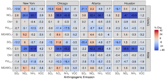
Figure 3.
Comparison of the percent change in pollutant concentrations for four urban CBSAs during January 2016 as predicted by the pf-RSM and CMAQ. Units: ppb for MDA8 ozone and μg m−3 for PM2.5 and its components.
Comparisons of mean absolute concentrations predicted by the pf-RSM and CMAQ over all CBSAs in the domain for 0% to 100% emission reductions in January 2016 are provided in Figure 4. The predictions discussed above for the 60% emission reductions are generally reflective of the model response indicated in Figure 4, although the disbenefits in MDA8 ozone for 60% NOx emission reductions transition to benefits for larger reductions. For instance, MDA8 ozone increased over the CBSAs by 0.7 ppb for the 40% NOx emission reduction but decreased by 2.8 ppb for the 100% NOx reduction in the CMAQ simulations.
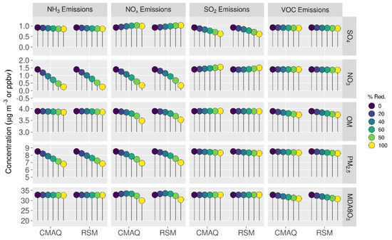
Figure 4.
Comparison of the mean absolute concentrations predicted by the pf-RSM and CMAQ over all CBSAs in the domain during January 2016 for U.S. anthropogenic emission changes from 0 to 100%. Units: ppbv for MDA8 ozone and μg m−3 for PM2.5 and its components.
The trend of increasing sulfate with decreasing NOx emissions (Figure 4) is consistent with Shah et al. [52], who reported that the SO2-to-sulfate conversion efficiency increased from 0.11 to 0.18 in winter in the eastern U.S. due to emission reductions during the 2007–2015 period. For CMAQ predictions, the trend of increasing sulfate with decreasing NOx emissions reverses for NOx reductions greater than about 80% but continues for the pf-RSM. pf-RSM performance could be improved for this case by including additional simulations in model fitting [19], although there could also be limitations in the polynomial functions for representing the entire range of concentration response. Nevertheless, the pf-RSM generally captures the CMAQ responses across species and emission changes, including the overall response in PM2.5 concentrations. CMAQ predictions of changes in mean PM2.5 concentrations over the CBSAs for 100% reductions in anthropogenic emissions are −1.72 μg m−3 (−20%, NH3 emissions); −1.61 μg m−3 (−19%, NOx emissions); and −0.19 μg m−3 (−2.2%, SO2 and VOC emissions). The PM2.5 concentration reductions associated with 100% NOx emission reductions overcome a 0.07 μg m−3 sulfate disbenefit, and the PM2.5 concentration reductions for 100% SO2 emission reductions overcome a 0.15 μg m−3 nitrate disbenefit (about 50% of the sulfate reduction in that case).
3.2. July
The mean concentration responses in July 2016 predicted by the pf-RSM and CMAQ are compared for the 30 OOS cases in Figure 5. The pf-RSM predictions for MDA8 ozone agree well with CMAQ results across the full set of OOS simulations, even for the case of 100% NOx emission reductions with large (>30 ppb) MDA8 ozone decreases (Supplementary Figure S6). Nitrate responses are also in general agreement for the pf-RSM and CMAQ, although the pf-RSM tends to underestimate the magnitude of the disbenefits predicted by CMAQ. These underestimates are associated with the 100% SO2 emission reduction simulation (Supplementary Figure S7).
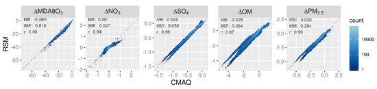
Figure 5.
Comparison of changes in mean July concentrations predicted by the pf-RSM and 30 OOS CMAQ simulations. Units: ppb for MDA8 ozone and μg m−3 for PM2.5 and its components.
For the sulfate response, a forked pattern exists in the scatterplot for concentration decreases larger than 1 μg m−3. This pattern results from pf-RSM underestimates of the CMAQ response for the 100% SO2 emission reduction case and overestimates for the Run 5 case. The forked pattern for the OM response is due to pf-RSM response overestimates for the 80% and 100% NOx emission reduction cases and slight underestimates for the Run 5 case. Moreover, the OM disbenefits predicted by CMAQ were underestimated by the pf-RSM for the 100% NH3 emission reduction case (Supplementary Figure S9). The forked pattern in the scatterplot for the PM2.5 response as well as the pf-RSM underestimate of PM2.5 disbenefits follows the behavior for OM (i.e., PM2.5 responses are overestimated for the 100% NOx emission reductions and disbenefits are underestimated for 100% NH3 emission reductions, Supplementary Figure S10).
In Figure 6, the spatial patterns of concentration responses in July 2016 are compared for CMAQ and the pf-RSM for MDA8 ozone, nitrate, sulfate, and OM for 60% reductions in NH3, NOx, SO2, and VOC emissions. The pf-RSM and CMAQ response patterns are generally in good agreement across cases. For MDA8 ozone, the 60% NOx emission reductions lead to large ozone decreases (mean: 7 ppb) throughout the eastern U.S. (Figure 6a), in contrast to the ozone increases predicted in January in northern and urban areas. Emission reductions for other species have a relatively small effect on MDA8 ozone. The 60% reductions in NOx and NH3 emissions reduce nitrate concentrations through a band of cells from Iowa to Pennsylvania, and NOx emissions reductions also reduce nitrate in parts of Florida (Figure 6b). The SO2 emission reductions cause increases in nitrate concentrations in some areas, likely due to chemical feedbacks of acidity on gas-particle partitioning of total nitrate. NOx and NH3 emission reductions lead to small sulfate decreases due to the influence of NOx on oxidant abundance and NH3 on cloud pH. SO2 reductions reduce sulfate in the Ohio Valley where large SO2 sources are located (Figure 6c).
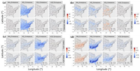
Figure 6.
Comparison of the change in average concentration in July 2016 for the pf-RSM and CMAQ for a 60% reduction in anthropogenic emissions of NH3, NOx, SO2, and VOC: (a) MDA8 ozone, (b) PM2.5 nitrate, (c) PM2.5 sulfate, and (d) PM2.5 OM. Units: ppb for MDA8 ozone and μg m−3 for PM2.5 components. Statistics for pf-RSM and CMAQ comparison: MB: mean bias; 98E: 98th percentile of error; r: Pearson correlation coefficient.
The 60% reductions in NH3 emissions increase OM concentrations along a latitude band between 32 N and 42 N. This behavior appears to be associated with biogenic SOA formation from acid-catalyzed uptake of isoprene epoxydiols (IEPOX) and subsequent in-particle reaction involving nucleophile addition to the parent hydrocarbon. This SOA formation pathway is enhanced under conditions of greater acidity and increased nucleophile (water and sulfate) concentration (i.e., eqn. 4 of Pye et al. [57]). The 60% reduction in NH3 emissions reduces pH by 0.23 on average (up to 0.84) (Figure 7a), which corresponds to a 75% increase in [H+] on average (up to 594%). These increases in acidity rather than changes in nucleophile concentrations explain the OM concentration increases, because sulfate concentrations decrease with decreasing NH3 emissions (Figure 6c) and aerosol water concentrations also generally decrease, except over a region around West Virginia with small (<9%) increases (Figure 7b).
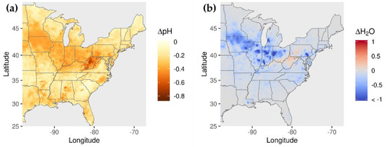
Figure 7.
Change in (a) pH and (b) fine-particle water concentration for 60% reduction in NH3 emissions.
The 60% reductions in NOx emissions decrease OM concentrations in the southern U.S. where biogenic SOA is relatively high (Figure 6d). Previous work has found that reducing NOx in the southeast U.S. in summer leads to substantial reductions in the organic nitrate fraction of OM and smaller changes for other OM contributors [55]. SO2 emission reductions reduce OM concentrations with a spatial pattern similar to that previously reported for the SO2 response of biogenic SOA formed via aerosol water chemistry [58]. As described above, SO2 emission reductions can reduce particle acidity and nucleophile concentrations and thereby lower biogenic SOA production. Anthropogenic VOC emission reductions lead to small OM concentration reductions in the CMAQ simulations, but the pf-RSM predicts small increases. This behavior did not occur in previous pf-RSM applications in China and should be investigated further in future studies.
Good agreement exists between pf-RSM and CMAQ predictions of the percent change in concentrations over the four CBSAs in Figure 8 for 60% reductions in precursor emissions in July. In response to the SO2 emission reductions, sulfate concentrations decreased by 0.1 μg m−3 in Houston, 0.25 μg m−3 in Atlanta, 0.28 μg m−3 in NY, and 0.38 μg m−3 in Chicago. In contrast, the SO2 emission reductions caused some increases in nitrate concentrations, although the effect is small (0.02 μg m−3 in Houston and Atlanta, 0.03 μg m−3 in NY, and 0.09 μg m−3 in Chicago) due to the low nitrate concentrations in summer. In response to 60% NOx emission reductions, MDA8 ozone concentrations decreased from 16% (5 ppb in Houston) to 28% (12 ppb in Atlanta) in the CMAQ simulations. NOx emission reductions also caused decreases in OM concentrations in the CBSAs, with the greatest reduction in Atlanta (18%, 1.5 μg m−3), where biogenic SOA is prominent. NOx emission reductions caused large percent reductions in nitrate concentrations (up to 36% in Chicago), but the absolute concentration changes are small (i.e., ≤0.12 μg m−3). NH3 emission reductions lead to decreases in nitrate concentrations and increases in OM concentrations in July. The OM increases are greater than the nitrate decreases in absolute terms (greater by 0.14 μg m−3 in NY, 0.03 μg m−3 in Chicago, 0.23 μg m−3 in Atlanta, and 0.02 μg m−3 in Houston). Anthropogenic VOC reductions have a small effect on concentrations in July due to the high levels of biogenic VOC, although this study did not consider intermediate and semi-volatile VOC beyond what is included in the NEI.
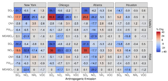
Figure 8.
Comparison of the percent change in pollutant concentrations for four urban CBSAs during July 2016 as predicted by the pf-RSM and CMAQ. Units: ppb for MDA8 ozone and μg m−3 for PM2.5 and its components.
Comparisons of mean absolute concentrations predicted by the pf-RSM and CMAQ over all CBSAs in the domain for 0% to 100% emission reductions in July 2016 are shown in Figure 9. SO2 emission reductions reduce sulfate (up to 0.42 μg m−3) and OM (up to 0.16 μg m−3) concentrations but increase nitrate concentrations (up to 0.13 μg m−3). In contrast to January, NOx emission reductions reduce MDA8 ozone and sulfate concentrations for all NOx emission reduction levels due to the greater oxidant abundance in July. NOx emission reductions also decrease OM concentrations (up to 0.93 μg m−3). NH3 emission reductions lead to increases in OM concentrations (up to 0.51 μg m−3), with increases growing nonlinearly with a decreasing emission level. As discussed above, the fact that OM concentration increases with decreasing NH3 emissions could be related to biogenic SOA formation associated with IEPOX uptake. Additional investigation of this SOA formation pathway under low NH3 and SO2 (and water content) conditions would be worthwhile. Riva et al. [59] reported that IEPOX organosulfates are highly viscous and likely to lead to phase separation under acidic conditions with low water content. Phase separation becomes more likely as sulfate decreases relative to IEPOX, resulting in increased diffusion barriers to further IEPOX uptake and SOA formation. Such behavior, which is not present in the base CMAQ model, could affect the sensitivity of OM to SO2 and NH3 emissions.
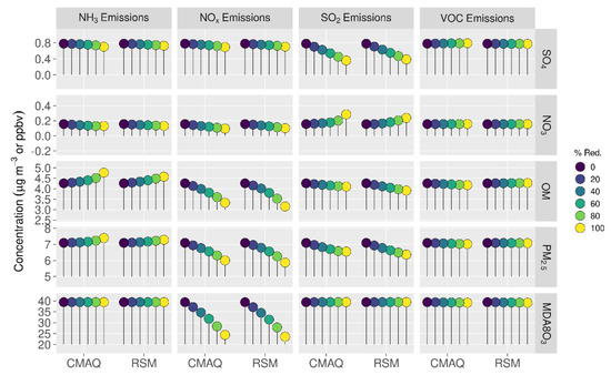
Figure 9.
Comparison of the mean absolute concentrations predicted by the pf-RSM and CMAQ over all CBSAs in the domain during July 2016 for U.S. anthropogenic emission changes from 0 to 100%. Units: ppbv for MDA8 ozone and μg m−3 for PM2.5 and its components.
Predicted changes in PM2.5 concentrations for 100% reductions in anthropogenic emissions are −1.09 μg m−3 (−15.4%) (NOx emissions); −0.54 μg m−3 (−7.67%) (SO2 emissions); −0.072 μg m−3 (−1.02%) (VOC emissions); and +0.30 μg m−3 (+4.3%) (NH3 emissions). The PM2.5 concentration decreases associated with 100% NOx emission reductions include a small decrease in sulfate concentration of 0.09 μg m−3 (in contrast to January when sulfate concentrations increased with NOx emission reductions). The PM2.5 concentration decreases for 100% SO2 emission reductions overcome a 0.13 μg m−3 increase in nitrate concentration (about 30% of the sulfate concentration decrease, 0.42 μg m−3). The predicted change in MDA8 ozone concentration for 100% reduction in NOx emissions is −15.0 ppb (38%), and for 100% reduction in VOC emissions, it is 0.25 ppb.
4. Conclusions
Reducing PM2.5 and ozone concentrations is important to protect human health and the environment. CTMs are valuable tools for exploring policy options for improving air quality, but CTMs are computationally expensive and statistical models are therefore developed to approximate CTMs in some applications. Recent developments in RSM technology have reduced the number of CTM simulations needed for model fitting and provide an opportunity to evaluate RSM performance in the U.S.
Predictions of the pf-RSM developed here are in good agreement with OOS CMAQ simulations in the eastern U.S., with some exceptions for cases with anthropogenic emission reductions approaching 100%. These extreme conditions may have limited relevance in typical applications. Furthermore, previous work [19] suggests that performance can be improved in these cases by including additional simulations in pf-RSM fitting. Although the pf-RSM required fewer simulations for development than previous-generation RSMs, the one-region, five-emission factor pf-RSM still required about 20 CTM simulations. Therefore, computational expense would present challenges for developing pf-RSMs for multiple regions and emission sectors in typical applications. The recently developed DeepRSM approach [22], which requires fewer CTM simulations for fitting and improves performance compared with the pf-RSM, could facilitate the development of more complex RSMs in the future.
NOx emission reductions were more effective for reducing PM2.5 concentrations than SO2, NH3, and traditional VOC emission reductions. In January, NOx emission reductions decreased nitrate concentrations in the north and OM concentrations in the south. NOx emission reductions did cause some disbenefits for sulfate concentrations in January, but the decreases in other PM2.5 components overcame the disbenefits. In July, NOx emission reductions led to substantial decreases in OM concentrations by reducing biogenic SOA formation in the south. NH3 emission reductions were effective for reducing nitrate concentrations in January but increased OM concentrations in July. As a result, the effectiveness of NH3 emission reductions for reducing PM2.5 concentrations was less than for NOx emission reductions overall. More work should be done to understand IEPOX SOA formation under conditions of low NH3 emissions to verify the OM responses predicted here. VOC emission reductions had a smaller effect on PM2.5 concentrations than NOx and NH3 in part due to high levels of biogenic VOC in the eastern U.S. Moreover, our study did not include emissions of intermediate and semi-volatile VOC [36] beyond what is included in the NEI.
For MDA8 ozone concentrations, large reductions (>80%) in NOx emissions are needed to avoid disbenefits in northern and urban areas in January. In July, all levels of NOx emission reductions are effective for reducing MDA8 ozone due to the abundance of oxidants in summer. VOC emission reductions caused small decreases in MDA8 ozone concentrations in January and had little effect in July due to the high levels of biogenic VOC.
Since our study focused on the nonlinear response of pollutant concentrations, we did not discuss the influence of primary PM2.5 emissions on PM2.5 concentrations. However, PM2.5 concentrations are generally more responsive to reductions in primary PM2.5 emissions than the precursors for secondary PM2.5 discussed here. Some components of primary PM2.5 emissions (e.g., crustal cations) can also influence concentrations of secondary PM2.5 [60,61]. Large reductions in NOx and SO2 emissions in the eastern U.S. in recent decades have reduced the concentrations of secondary inorganic aerosol and increased the importance of primary PM2.5 emissions and organic aerosol. Improved representations of the emissions and chemistry of organic aerosol are increasingly important in this context.
Supplementary Materials
The following are available online at https://www.mdpi.com/article/10.3390/atmos12081044/s1, Table S1: CMAQ model performance statistics, Table S2: Definition of statistics used in the CMAQ model performance evaluation, Table S3: Fractional change in U.S. anthropogenic emissions for simulations used in developing the pf-RSM, Table S4: Fractional change in U.S. anthropogenic emissions for 30 OOS simulations used in evaluating the pf-RSM, Figure S1–S5: Comparison of changes in mean January species concentrations predicted by the pf-RSM and 30 OOS CMAQ simulations, Figures S6–S10: Comparison of changes in mean July species concentrations predicted by the pf-RSM and 30 OOS CMAQ simulations.
Author Contributions
Conceptualization, J.T.K. and C.J.; methodology, J.T.K. and C.J.; software, C.J., Y.Z., S.L., J.X., S.W. and B.N.M.; validation, J.T.K., C.J. and S.L.; writing—original draft preparation, J.T.K.; writing—review and editing, J.T.K., C.J., Y.Z., S.L., J.X., S.W., B.N.M. and H.O.T.P.; visualization, J.T.K.; project administration, J.T.K. and C.J. All authors have read and agreed to the published version of the manuscript.
Funding
This research received no external funding.
Institutional Review Board Statement
Not applicable.
Informed Consent Statement
Not applicable.
Data Availability Statement
Publicly available datasets were analyzed in this study. This data can be found here: ftp://newftp.epa.gov/aqmg/cjang/RSM/RSM-VAT2.6/.
Acknowledgments
The authors thank Kristen Foley and Shannon Koplitz for helpful comments on a draft version of this article.
Conflicts of Interest
The authors declare no conflict of interest.
Disclaimer
The views expressed in this manuscript are those of the authors alone and do not necessarily reflect the views and policies of the U.S. Environmental Protection Agency.
References
- USEPA. Integrated Science Assessment (ISA) for Particulate Matter (Final Report, 2019); EPA/600/R-19/188; U.S. Environmental Protection Agency: Washington, DC, USA, 2019.
- USEPA. Integrated Science Assessment (ISA) for Ozone and Related Photochemical Oxidants (Final Report, April 2020); EPA/600/R-20/012; U.S. Environmental Protection Agency: Washington, DC, USA, 2020.
- SJVAPCD. San Joaquin Valley Air Pollution Control District, 2018 Plan for the 1997, 2006, and 2012 PM2.5 Standards. 2018. Available online: http://valleyair.org/pmplans/documents/2018/pm-plan-adopted/2018-Plan-for-the-1997-2006-and-2012-PM2.5-Standards.pdf (accessed on 11 August 2021).
- Allegheny County Health Department (ACHD). Revision to the Allegheny County Portion of the Pennsylvania State Implementation Plan. Attainment Demonstration for the Allegheny County, PA PM2.5 Nonattainment Area, 2012 NAAQS. 2019. Available online: https://alleghenycounty.us/uploadedFiles/Allegheny_Home/Health_Department/Programs/Air_Quality/SIPs/90-SIP-PM25-ATTAIN-2012-NAAQS-09-12-2019.pdf (accessed on 11 August 2021).
- Bachmann, J. Will the Circle Be Unbroken: A History of the U.S. National Ambient Air Quality Standards. J. Air Waste Manag. Assoc. 2007, 57, 652–697. [Google Scholar] [CrossRef] [PubMed]
- USEPA. Modeling Guidance for Demonstrating Attainment of Air Quality Goals for Ozone, PM2.5, and Regional Haze; EPA -454/B-07-002 U.S. EPA, Office of Air Quality Planning and Standards. Research Triangle Park, NC. EPA 454/R-18-009. 2018. Available online: https://www.epa.gov/sites/default/files/2020-10/documents/o3-pm-rh-modeling_guidance-2018.pdf (accessed on 11 August 2021).
- Finlayson-Pitts, B.J.; Pitts, J.N. Chemistry of the Upper and Lower Atmosphere: Theory, Experiments and Applications; Academic Press: Cambridge, MA, USA, 2000. [Google Scholar]
- Ansari, A.S.; Pandis, S.N. Response of Inorganic PM to Precursor Concentrations. Environ. Sci. Technol. 1998, 32, 2706–2714. [Google Scholar] [CrossRef]
- Pye, H.O.T.; Nenes, A.; Alexander, B.; Ault, A.P.; Barth, M.C.; Clegg, S.L.; Collett, J.L., Jr.; Fahey, K.M.; Hennigan, C.J.; Herrmann, H.; et al. The acidity of atmospheric particles and clouds. Atmos. Chem. Phys. 2020, 20, 4809–4888. [Google Scholar] [CrossRef] [PubMed] [Green Version]
- Womack, C.C.; McDuffie, E.E.; Edwards, P.M.; Bares, R.; de Gouw, J.A.; Docherty, K.S.; Dubé, W.P.; Fibiger, D.L.; Franchin, A.; Gilman, J.B.; et al. An Odd Oxygen Framework for Wintertime Ammonium Nitrate Aerosol Pollution in Urban Areas: NOx and VOC Control as Mitigation Strategies. Geophys. Res. Lett. 2019, 46, 4971–4979. [Google Scholar] [CrossRef] [Green Version]
- Kleeman, M.J.; Ying, Q.; Kaduwela, A. Control strategies for the reduction of airborne particulate nitrate in California’s San Joaquin Valley. Atmos. Environ. 2005, 39, 5325–5341. [Google Scholar] [CrossRef]
- Thunis, P.; Clappier, A.; Beekmann, M.; Putaud, J.P.; Cuvelier, C.; Madrazo, J.; de Meij, A. Non-linear response of PM2.5 to changes in NOx and NH3 emissions in the Po basin (Italy): Consequences for air quality plans. Atmos. Chem. Phys. Discuss. 2021, 2021, 1–26. [Google Scholar] [CrossRef]
- West, J.J.; Ansari, A.S.; Pandis, S.N. Marginal PM2.5: Nonlinear Aerosol Mass Response to Sulfate Reductions in the Eastern United States. J. Air Waste Manag. Assoc. 1999, 49, 1415–1424. [Google Scholar] [CrossRef] [Green Version]
- Simon, H.; Reff, A.; Wells, B.; Xing, J.; Frank, N. Ozone Trends Across the United States over a Period of Decreasing NOx and VOC Emissions. Environ. Sci. Technol. 2015, 49, 186–195. [Google Scholar] [CrossRef] [Green Version]
- Huang, J.; Zhu, Y.; Kelly, J.T.; Jang, C.; Wang, S.; Xing, J.; Chiang, P.-C.; Fan, S.; Zhao, X.; Yu, L. Large-scale optimization of multi-pollutant control strategies in the Pearl River Delta region of China using a genetic algorithm in machine learning. Sci. Total Environ. 2020, 722, 137701. [Google Scholar] [CrossRef]
- Xing, J.; Wang, S.; Jang, C.J.; Zhu, Y.; Zhao, B.; Ding, D.; Wang, J.; Zhao, L.; Xie, H.; Hao, J. An Overview of the Air Pollution Control Cost–Benefit and Attainment Assessment System and Its Application in China. The Magazine for Environmental Managers. April 2017. Available online: https://pubs.awma.org/flip/EM-Apr-2017/xing.pdf (accessed on 11 August 2021).
- Zhang, F.; Xing, J.; Zhou, Y.; Wang, S.; Zhao, B.; Zheng, H.; Zhao, X.; Chang, H.; Jang, C.; Zhu, Y.; et al. Estimation of abatement potentials and costs of air pollution emissions in China. J. Environ. Manag. 2020, 260, 110069. [Google Scholar] [CrossRef]
- Heo, J.; Adams, P.J.; Gao, H.O. Reduced-form modeling of public health impacts of inorganic PM2.5 and precursor emissions. Atmos. Environ. 2016, 137, 80–89. [Google Scholar] [CrossRef]
- Xing, J.; Ding, D.; Wang, S.; Zhao, B.; Jang, C.; Wu, W.; Zhang, F.; Zhu, Y.; Hao, J. Quantification of the enhanced effectiveness of NOx control from simultaneous reductions of VOC and NH3 for reducing air pollution in the Beijing–Tianjin–Hebei region, China. Atmos. Chem. Phys. 2018, 18, 7799–7814. [Google Scholar] [CrossRef] [Green Version]
- Xing, J.; Wang, S.; Zhao, B.; Wu, W.; Ding, D.; Jang, C.; Zhu, Y.; Chang, X.; Wang, J.; Zhang, F.; et al. Quantifying Nonlinear Multiregional Contributions to Ozone and Fine Particles Using an Updated Response Surface Modeling Technique. Environ. Sci. Technol. 2017, 51, 11788–11798. [Google Scholar] [CrossRef] [PubMed]
- Xing, J.; Wang, S.X.; Jang, C.; Zhu, Y.; Hao, J.M. Nonlinear response of ozone to precursor emission changes in China: A modeling study using response surface methodology. Atmos. Chem. Phys. 2011, 11, 5027–5044. [Google Scholar] [CrossRef] [Green Version]
- Xing, J.; Zheng, S.; Ding, D.; Kelly, J.T.; Wang, S.; Li, S.; Qin, T.; Ma, M.; Dong, Z.; Jang, C.; et al. Deep Learning for Prediction of the Air Quality Response to Emission Changes. Environ. Sci. Technol. 2020, 54, 8589–8600. [Google Scholar] [CrossRef]
- Wang, S.; Xing, J.; Jang, C.; Zhu, Y.; Fu, J.S.; Hao, J. Impact Assessment of Ammonia Emissions on Inorganic Aerosols in East China Using Response Surface Modeling Technique. Environ. Sci. Technol. 2011, 45, 9293–9300. [Google Scholar] [CrossRef] [PubMed]
- Zhao, B.; Wang, S.X.; Xing, J.; Fu, K.; Fu, J.S.; Jang, C.; Zhu, Y.; Dong, X.Y.; Gao, Y.; Wu, W.J.; et al. Assessing the nonlinear response of fine particles to precursor emissions: Development and application of an extended response surface modeling technique v1.0. Geosci. Model Dev. 2015, 8, 115–128. [Google Scholar] [CrossRef] [Green Version]
- Zhao, B.; Wu, W.; Wang, S.; Xing, J.; Chang, X.; Liou, K.N.; Jiang, J.H.; Gu, Y.; Jang, C.; Fu, J.S.; et al. A modeling study of the nonlinear response of fine particles to air pollutant emissions in the Beijing–Tianjin–Hebei region. Atmos. Chem. Phys. 2017, 17, 12031–12050. [Google Scholar] [CrossRef] [Green Version]
- Foley, K.M.; Napelenok, S.L.; Jang, C.; Phillips, S.; Hubbell, B.J.; Fulcher, C.M. Two reduced form air quality modeling techniques for rapidly calculating pollutant mitigation potential across many sources, locations and precursor emission types. Atmos. Environ. 2014, 98, 283–289. [Google Scholar] [CrossRef]
- Tessum, C.W.; Hill, J.D.; Marshall, J.D. InMAP: A model for air pollution interventions. PLoS ONE 2017, 12, e0176131. [Google Scholar] [CrossRef]
- USEPA. Technical Support Document for the Proposed PM NAAQS Rule: Response Surface Modeling; Office of Air Quality Planning and Standards, US Environmental Protection Agency: Research Triangle Park, NC, USA, 2006; p. 48.
- USEPA. Technical Support Document for the Proposed Mobile Source Air Toxics Rule: Ozone Modeling; Office of Air Quality Planning and Standards, US Environmental Protection Agency: Research Triangle Park, NC, USA, 2006; p. 49.
- Xing, J.; Ding, D.; Wang, S.; Dong, Z.; Kelly, J.T.; Jang, C.; Zhu, Y.; Hao, J. Development and application of observable response indicators for design of an effective ozone and fine-particle pollution control strategy in China. Atmos. Chem. Phys. 2019, 19, 13627–13646. [Google Scholar] [CrossRef] [Green Version]
- Emery, C.; Jung, J.; Koo, B.; Yarwood, G. Improvements to CAMx Snow Cover Treatments and Carbon Bond Chemical Mechanism for Winter Ozone; Final Report; Utah Department of Environmental Quality: Salt Lake City, UT, USA; Ramboll Environ: Novato, CA, USA, 2015.
- Appel, K.W.; Napelenok, S.L.; Foley, K.M.; Pye, H.O.T.; Hogrefe, C.; Luecken, D.J.; Bash, J.O.; Roselle, S.J.; Pleim, J.E.; Foroutan, H.; et al. Description and evaluation of the Community Multiscale Air Quality (CMAQ) modeling system version 5.1. Geosci. Model Dev. 2017, 10, 1703–1732. [Google Scholar] [CrossRef] [PubMed] [Green Version]
- Simon, H.; Bhave, P.V. Simulating the Degree of Oxidation in Atmospheric Organic Particles. Environ. Sci. Technol. 2012, 46, 331–339. [Google Scholar] [CrossRef] [PubMed]
- Mathur, R.; Xing, J.; Gilliam, R.; Sarwar, G.; Hogrefe, C.; Pleim, J.; Pouliot, G.; Roselle, S.; Spero, T.L.; Wong, D.C.; et al. Extending the Community Multiscale Air Quality (CMAQ) modeling system to hemispheric scales: Overview of process considerations and initial applications. Atmos. Chem. Phys. 2017, 17, 12449–12474. [Google Scholar] [CrossRef] [PubMed] [Green Version]
- USEPA. Technical Support Document (TSD) Preparation of Emissions Inventories for 2016v1 North American Emissions Modeling Platform. 2020. Available online: https://www.epa.gov/air-emissions-modeling/2016-version-1-technical-support-document (accessed on 11 August 2021).
- Murphy, B.N.; Woody, M.C.; Jimenez, J.L.; Carlton, A.M.G.; Hayes, P.L.; Liu, S.; Ng, N.L.; Russell, L.M.; Setyan, A.; Xu, L.; et al. Semivolatile POA and parameterized total combustion SOA in CMAQv5.2: Impacts on source strength and partitioning. Atmos. Chem. Phys. 2017, 17, 11107–11133. [Google Scholar] [CrossRef] [Green Version]
- Bash, J.O.; Baker, K.R.; Beaver, M.R. Evaluation of improved land use and canopy representation in BEIS v3.61 with biogenic VOC measurements in California. Geosci. Model Dev. 2016, 9, 2191–2207. [Google Scholar] [CrossRef] [Green Version]
- Gantt, B.; Kelly, J.T.; Bash, J.O. Updating sea spray aerosol emissions in the Community Multiscale Air Quality (CMAQ) model version 5.0.2. Geosci. Model Dev. 2015, 8, 3733–3746. [Google Scholar] [CrossRef] [Green Version]
- USEPA. Meteorological Model Performance for Annual 2016 Simulation WRF v3.8. 2019. Available online: https://www.epa.gov/sites/production/files/2020-10/documents/met_model_performance-2016_wrf.pdf (accessed on 11 August 2021).
- Kelly, J.T.; Koplitz, S.N.; Baker, K.R.; Holder, A.L.; Pye, H.O.T.; Murphy, B.N.; Bash, J.O.; Henderson, B.H.; Possiel, N.C.; Simon, H.; et al. Assessing PM2.5 model performance for the conterminous U.S. with comparison to model performance statistics from 2007-2015. Atmos. Environ. 2019, 214, 116872. [Google Scholar] [CrossRef]
- Simon, H.; Baker, K.R.; Phillips, S. Compilation and interpretation of photochemical model performance statistics published between 2006 and 2012. Atmos. Environ. 2012, 61, 124–139. [Google Scholar] [CrossRef]
- Appel, K.W.; Bash, J.O.; Fahey, K.M.; Foley, K.M.; Gilliam, R.C.; Hogrefe, C.; Hutzell, W.T.; Kang, D.; Mathur, R.; Murphy, B.N.; et al. The Community Multiscale Air Quality (CMAQ) Model Versions 5.3 and 5.3.1: System Updates and Evaluation. Geosci. Model Dev. Discuss. 2020, 2020, 1–41. [Google Scholar] [CrossRef]
- Hammersley, J.M. Monte Carlo Methods for Solving Multivariable Problems. Ann. N. Y. Acad. Sci. 1960, 86, 844–874. [Google Scholar] [CrossRef]
- Murphy, B.N.; Nolte, C.G.; Sidi, F.; Bash, J.O.; Appel, K.W.; Jang, C.; Kang, D.; Kelly, J.; Mathur, R.; Napelenok, S.; et al. The Detailed Emissions Scaling, Isolation, and Diagnostic (DESID) module in the Community Multiscale Air Quality (CMAQ) Modeling System version 5.3. Geosci. Model Dev. Discuss. 2020, 2020, 1–28. [Google Scholar] [CrossRef]
- Jin, J.; Zhu, Y.; Jang, J.; Wang, S.; Xing, J.; Chiang, P.-C.; Fan, S.; Long, S. Enhancement of the polynomial functions response surface model for real-time analyzing ozone sensitivity. Front. Environ. Sci. Eng. 2020, 15, 31. [Google Scholar] [CrossRef]
- Jacob, D.J.; Horowitz, L.W.; Munger, J.W.; Heikes, B.G.; Dickerson, R.R.; Artz, R.S.; Keene, W.C. Seasonal transition from NOx- to hydrocarbon-limited conditions for ozone production over the eastern United States in September. J. Geophys. Res. Atmos. 1995, 100, 9315–9324. [Google Scholar] [CrossRef]
- Martin, R.V.; Fiore, A.M.; Van Donkelaar, A. Space-based diagnosis of surface ozone sensitivity to anthropogenic emissions. Geophys. Res. Lett. 2004, 31, L06120. [Google Scholar] [CrossRef] [Green Version]
- Wang, R.; Guo, X.; Pan, D.; Kelly, J.T.; Bash, J.O.; Sun, K.; Paulot, F.; Clarisse, L.; Van Damme, M.; Whitburn, S.; et al. Monthly Patterns of Ammonia Over the Contiguous United States at 2-km Resolution. Geophys. Res. Lett. 2021, 48, e2020GL090579. [Google Scholar] [CrossRef]
- Nenes, A.; Pandis, S.N.; Weber, R.J.; Russell, A. Aerosol pH and liquid water content determine when particulate matter is sensitive to ammonia and nitrate availability. Atmos. Chem. Phys. 2020, 20, 3249–3258. [Google Scholar] [CrossRef] [Green Version]
- Guo, H.; Sullivan, A.P.; Campuzano-Jost, P.; Schroder, J.C.; Lopez-Hilfiker, F.D.; Dibb, J.E.; Jimenez, J.L.; Thornton, J.A.; Brown, S.S.; Nenes, A.; et al. Fine particle pH and the partitioning of nitric acid during winter in the northeastern United States. J. Geophys. Res. Atmos. 2016, 121, 10–355. [Google Scholar] [CrossRef]
- Seinfeld, J.H.; Pandis, S.N. Atmospheric Chemistry and Physics: From Air Pollution to Climate Change, 3rd ed.; John Wiley & Sons: New York, NY, USA, 2016. [Google Scholar]
- Shah, V.; Jaeglé, L.; Thornton, J.A.; Lopez-Hilfiker, F.D.; Lee, B.H.; Schroder, J.C.; Campuzano-Jost, P.; Jimenez, J.L.; Guo, H.; Sullivan, A.P.; et al. Chemical feedbacks weaken the wintertime response of particulate sulfate and nitrate to IEPOXs over the eastern United States. Proc. Natl. Acad. Sci. USA 2018, 115, 8110–8115. [Google Scholar] [CrossRef] [Green Version]
- Xu, L.; Pye, H.O.T.; He, J.; Chen, Y.; Murphy, B.N.; Ng, N.L. Experimental and model estimates of the contributions from biogenic monoterpenes and sesquiterpenes to secondary organic aerosol in the southeastern United States. Atmos. Chem. Phys. 2018, 18, 12613–12637. [Google Scholar] [CrossRef] [PubMed] [Green Version]
- Henze, D.K.; Seinfeld, J.H.; Ng, N.L.; Kroll, J.H.; Fu, T.M.; Jacob, D.J.; Heald, C.L. Global modeling of secondary organic aerosol formation from aromatic hydrocarbons: High- vs. low-yield pathways. Atmos. Chem. Phys. 2008, 8, 2405–2420. [Google Scholar] [CrossRef] [Green Version]
- Pye, H.O.T.; Luecken, D.J.; Xu, L.; Boyd, C.M.; Ng, N.L.; Baker, K.R.; Ayres, B.R.; Bash, J.O.; Baumann, K.; Carter, W.P.L.; et al. Modeling the Current and Future Roles of Particulate Organic Nitrates in the Southeastern United States. Environ. Sci. Technol. 2015, 49, 14195–14203. [Google Scholar] [CrossRef] [PubMed]
- Pye, H.O.T.; D’Ambro, E.L.; Lee, B.H.; Schobesberger, S.; Takeuchi, M.; Zhao, Y.; Lopez-Hilfiker, F.; Liu, J.; Shilling, J.E.; Xing, J.; et al. Anthropogenic enhancements to production of highly oxygenated molecules from autoxidation. Proc. Natl. Acad. Sci. USA 2019, 116, 6641. [Google Scholar] [CrossRef] [Green Version]
- Pye, H.O.T.; Pinder, R.W.; Piletic, I.R.; Xie, Y.; Capps, S.L.; Lin, Y.-H.; Surratt, J.D.; Zhang, Z.; Gold, A.; Luecken, D.J.; et al. Epoxide Pathways Improve Model Predictions of Isoprene Markers and Reveal Key Role of Acidity in Aerosol Formation. Environ. Sci. Technol. 2013, 47, 11056–11064. [Google Scholar] [CrossRef]
- Carlton, A.G.; Pye, H.O.T.; Baker, K.R.; Hennigan, C.J. Additional Benefits of Federal Air-Quality Rules: Model Estimates of Controllable Biogenic Secondary Organic Aerosol. Environ. Sci. Technol. 2018, 52, 9254–9265. [Google Scholar] [CrossRef]
- Riva, M.; Chen, Y.; Zhang, Y.; Lei, Z.; Olson, N.E.; Boyer, H.C.; Narayan, S.; Yee, L.D.; Green, H.S.; Cui, T.; et al. Increasing Isoprene Epoxydiol-to-Inorganic Sulfate Aerosol Ratio Results in Extensive Conversion of Inorganic Sulfate to Organosulfur Forms: Implications for Aerosol Physicochemical Properties. Environ. Sci. Technol. 2019, 53, 8682–8694. [Google Scholar] [CrossRef]
- Vasilakos, P.; Russell, A.; Weber, R.; Nenes, A. Understanding nitrate formation in a world with less sulfate. Atmos. Chem. Phys. 2018, 18, 12765–12775. [Google Scholar] [CrossRef] [Green Version]
- Vasilakos, P.; Hu, Y.; Russell, A.; Nenes, A. Determining the Role of Acidity, Fate and Formation of IEPOX-Derived SOA in CMAQ. Atmosphere 2021, 12, 707. [Google Scholar] [CrossRef]
Publisher’s Note: MDPI stays neutral with regard to jurisdictional claims in published maps and institutional affiliations. |
© 2021 by the authors. Licensee MDPI, Basel, Switzerland. This article is an open access article distributed under the terms and conditions of the Creative Commons Attribution (CC BY) license (https://creativecommons.org/licenses/by/4.0/).