Visual Weather Property Prediction by Multi-Task Learning and Two-Dimensional RNNs

Abstract

We attempted to employ convolutional neural networks to extract visual features and developed recurrent neural networks for weather property estimation using only image data. Four common weather properties are estimated, i.e., temperature, humidity, visibility, and wind speed. Based on the success of previous works on temperature prediction, we extended them in terms of two aspects. First, by considering the effectiveness of deep multi-task learning, we jointly estimated four weather properties on the basis of the same visual information. Second, we propose that weather property estimations considering temporal evolution can be conducted from two perspectives, i.e., day-wise or hour-wise. A two-dimensional recurrent neural network is thus proposed to unify the two perspectives. In the evaluation, we show that better prediction accuracy can be obtained compared to the state-of-the-art models. We believe that the proposed approach is the first visual weather property estimation model trained based on multi-task learning.

1. Introduction

Visual attributes of images have been widely studied for years. Most previous works have focused on recognizing "explicit attributes" of images, such as object’s texture and color distribution [1], and semantic categories [2]. With the advancing of computer vision and machine learning technologies, more and more works have been proposed to study "implicit attributes" of images. These implicit attributes may not be represented in explicit forms, but are usually recognizable by human beings. For example, Lu et al. [3] proposed a method to recognize whether an image was captured on a sunny day or on a cloudy day. Hays and Efros [4] proposed to estimate geographic information from a single image (a.k.a IM2GPS). Recent research has demonstrated that deep learning approaches are effective for recognizing painting styles [5,6].

Among various implicit attributes, weather properties of images have attracted increasing attention. The earliest investigation of the relationship between vision and weather conditions dates back to early 2000s [7]. Thanks to the development of more advanced visual analysis and deep learning methods, a new wave of works studying the correlation between visual appearance and ambient temperature or other weather properties has recently emerged [8,9,10,11].

The main motivation of estimating weather properties from only images is that we could unveil characteristics in the real world from images available in cyberspace [11]. Images can be viewed as weather sensors [11], and by coupling estimated weather information with time/geographical information, explicit or implicit human behaviors can be discovered. Weather information can also be important priors for many computer vision applications. Figure 1 shows that the Eiffel Tower has drastically different visual appearances in different weather conditions, which brings significant challenges to object/landmark recognition. Once weather properties can be estimated, an object detector/recognizer can adapt for different weather conditions, so that the influences of visual variations can be reduced. The work in [12] shows that better understanding weather properties facilitates robust robotic vision. Models adaptive to weather conditions have been studied in lane detection and vehicle detection [13], and flying target detection [14]. The work in [15] also mentions that weather context may give clues for modeling the appearance of objects.

Weather property estimation can already be done by inexpensive sensors. Please notice that the proposed weather property estimation neither replaces nor improves existing weather sensors. We argue that analyzing images in cyberspace from the perspective of weather enables us to discover implicit human behaviors or to improve computer vision technologies to some extent.

Given outdoor images, in our previous work [10] we estimated ambient temperature based on visual information extracted from these images. Two application scenarios were proposed. The first one regards estimating the temperature of a given image regardless of temporal changes in the weather. The second scenario is, when several images of the same location over time are available, to "forecast" the temperature in the near future. In the first scenario, we extracted visual features using a convolutional neural network (CNN), and then used a regression layer outputting the estimated temperature. In the second scenario, features were also extracted using CNNs, but the temporal evolution was considered by recruiting a long-short term memory (LSTM) network, which output the estimated temperature of the last image in the given image sequence. This work is the state-of-the-art in temperature prediction from images.

On the basis of our previous work, in this study we made two significant improvements. First, we jointly estimated four weather properties, i.e., temperature, humidity, visibility, and wind speed, by a single network that was constructed based on the multi-task learning approach. These four properties can be estimated separately by four different models. However, the foundations for different estimations are the same, i.e., visual information extracted from images. Motivated by the success of deep multi-task learning [16], we attempted to construct a single network based on the multi-task learning approach and jointly handle four tasks. When training the network jointly for multiple tasks, different tasks may contribute complementary information to make the network more powerful.

When estimating temperature, previous works either take a single image as the input [9] or a sequence of images that were captured on different days [8,10]. For example, given the images captured on day i and day $i+1$, previous works estimated the temperature of the image captured on day $i+2$. In this work, we advocate that temporal evolution can be taken into account at different temporal scales. We can conduct day-wise estimation as mentioned above, or conduct hour-wise estimation as well. That is, given the images captured at hour j and hour $j+1$, which were captured on the same day i, we can estimate properties of the image captured at hour $j+2$. In addition, by considering different temporal scales together, we can mix day-wise and hour-wise estimation. For example, given the images captured at hour j and hour $j+1$ both captured on day i, we can estimate properties of the image captured at hour $j+1$ of day $i+1$. A two-dimensional RNN is thus proposed to implement this idea, which is the second improvement over [10].

Our contributions are summarized as follows.

• We adopted the multi-task learning approach to build a network that jointly estimates four weather properties based on features extracted by CNNs. We show that with multi-task learning, the proposed model outperforms single-task methods.
• We introduce a two-dimensional RNN to estimate weather properties at two temporal scales. To the best of our knowledge, this is the first deep learning model considering evolutions of appearance from two different perspectives.

The rest of this paper is organized as follows. Section 2 provides the literature survey. Section 3 presents data collection and data preprocessing. Section 4 presents a brief review of our previous work on single-task learning, and Section 5 provides details of the newly proposed multi-task learning approach. Various evaluation results and performance comparisons are given in Section 7, followed by the conclusion in Section 8.

2. Related Works

As a pioneering work studying visual manifestations of different weather conditions, Narasimhan and Nayar [7] discussed the relationships between visual appearance and weather conditions. Since then, several works have been proposed to work on weather type classification. Roser and Moosmann [17] focused on the images captured by cameras mounted on vehicles. They extracted features such as brightness, contrast, sharpness, and hue from sub-regions of an image, and concatenated them as an integrated vector. Based on these features, a classifier based on the support vector machine (SVM) was constructed to categorize images into clear, light rain, or heavy rain weather conditions. In [3], five types of weather features were designed, i.e., sky, shadow, reflection, contrast, and haze features. These features are not always present simultaneously. Therefore, a collaborative learning framework was proposed to dynamically weight the influences of different features and classify images into sunny or cloudy. Weather-specific features can be extracted from different perspectives, and conceptually they may be heterogeneous. In [11], a random forest classifier was proposed to integrate various types of visual features and classify images into one of five weather types, i.e., sunny, cloudy, snowy, rainy, or foggy. The merit of the random forest classifier is that it can handle heterogeneous types of features, and characteristics of the automatically determined decision trees imply the importance of different features. Kang et al. [18] used deep learning methods to recognizing weather types. They studied the performance of GoogLeNet and AlexNet when classifying images into hazy, rainy, or snowy. In this study, we also used deep learning models for visual weather analysis, but focused on weather property estimations.

In addition to weather type classification, more weather properties have also been investigated. Jacobs and his colleagues [19] initiated a project for collecting outdoor scene images captured by static webcams over a long period of time. The collected images formed the Archive of Many Outdoor Scenes (AMOS) dataset [19]. Based on the AMOS dataset, they proposed that webcams installed across the earth can be viewed as image sensors and enable us to understand weather patterns and variations over time [20]. More specifically, they adopted principal component analysis and canonical correlation analysis to predict wind velocity and vapor pressure from a sequence of images. Recently, Palvanov and Cho [21] focused on visibility estimation. They proposed a three-stream convolutional neural network to jointly consider different types of visibility features and handled images captured in different visibility ranges. Ibrahim et al. [22] developed the so-called WeatherNet that consists of four networks based on residual learning. These four networks were dedicated to recognize day/night, glare, precipitation, and fog. Similarly to [21], multiple separate networks were constructed to conduct dedicated tasks, and then results or intermediate information were fused together to estimate weather properties.

Laffont et al. [23] estimated scene attributes such as lighting, weather conditions, and seasons for images captured by webcams based on a set of regressors. Glasner et al. [8] studied the correlation between pixel intensity/camera motion and temperature and found a moderate correlation. With this observation, a regression model considering pixel intensity was constructed to predict temperature. Following the discussion in [8], Volokitin et al. [24] showed that, with appropriate fine tuning, deep features can be promising for temperature prediction. Zhou et al. [9] proposed a selective comparison learning scheme, and temperature prediction was conducted based on a CNN-based approach. Salman et al. [25] explored the correlations between different weather properties. In addition to considering temporal evolution, they proposed that, for example, visibility of an image can be better predicted if temperature and dew point are given in advance. Zhao et al. [26] argued that an image may be associated with multiple weather conditions; e.g., an image may present sunny but moist conditions. They thus proposed a CNN-RNN architecture to recognize weather conditions, and formulated this task as a multi-label problem. In this paper, we develop a multi-task learning approach considering temporal evolution to estimate weather properties. We propose that weather properties can be estimated from different temporal perspectives.

Aside from weather property estimations, Fedorov et al. [27] worked on an interesting application about snow. They extracted a set of visual features from images captured by webcams that monitored the target mountain, and then estimated the degree of snow cover by classifiers based on SVM, random forest, or logistic regression. In addition to visual analysis, some studies have been conducted from the perspective of text-based data analysis. Qiu et al. [28] proposed a deep learning-based method to predict rainfall based on weather features such as wind speed, air pressure, and temperature, collected from multiple surrounding observation sites.

In our previous work [10], we aimed at predicting temperature from a single image and forecasting the temperature of the last image in a given image sequence. Deep learning approaches were developed to consider temporal evolution of visual appearance. Unlike [8,9,24], we particularly advocate for the importance of modeling the temporal evolution via deep neural networks. Partially motivated by [21,22,25], we attempted to jointly consider the estimation of multiple weather properties in this paper. Instead of separately training multiple dedicated networks, we tried to develop a unified network for multiple tasks based on the multi-task learning scheme. Furthermore, we propose considering visual evolutions at different temporal scales. This idea is proposed for the first time for weather property estimations from visual appearance.

3. Data Collection and Processing

3.1. Datasets

The work in [10] verified that, by considering the temporal evolution of visual appearance, better temperature prediction performance can be achieved. Therefore, in this work we focused on predicting the temperature of the last image in an image sequence. For this task, the scene images mentioned in the Glasner dataset [8] were used as the seed. The Glasner dataset consists of images continuously captured by 10 cameras in 10 different environments (but all in USA) for two consecutive years. These cameras are in fact a small subset of the cameras used for the AMOS dataset [19], and from each of these ten cameras, the Glasner dataset only contains one image captured closest to 11 a.m. local time on each day. Notice that the ten cameras have different brands and in models, and thus images were captured based on various camera properties.

To build the proposed model, we needed more data for training. Therefore, according to the camera IDs mentioned in the Glasner dataset, we collected all their corresponding images from the AMOS dataset. In addition, according to the geographical information and the timestamp associated with each image, we obtained weather properties of each image from the cli-MATE website (http://mrcc.isws.illinois.edu/CLIMATE/, retrieved on 10 August 2018.). Overall, we collected 53,378 images from 9 cameras (one camera’s information was incorrect, and we could not successfully collect the corresponding weather properties) in total. We denote this dataset as Glasner-Exp in what follows.

Figure 2 shows one sample image of each of the nine scenes. We see that the scenes include a cityscape and a countryside in different weather conditions and seasons. Figure 3 shows three snapshots of each of the three scenes. The first two rows of Figure 3 shows two different image sequences of the same scene in the Glasner-Exp dataset. The first row shows images captured on 12 January, 13 January, and 14 January, and the second row shows images captured on 14 August, 15 August, and 16 August. We see that the visual appearance of images captured in the same scene may drastically vary due to climate. In addition, we clearly observe the temporal continuity of images captured on consecutive days. The third and fourth rows of Figure 3 show two more image sequences captured for different scenes.

3.2. Soft Classification vs. Regression

Intuitively, weather properties such as temperature are continuous values, and we can formulate the estimation task as a regression problem. However, we would like to describe the characteristics of the collected dataset, and point out that regression may not be a good way to handle this problem. First, the values collected from the cli-MATE website are discrete values, such as 25 °C, rather than 25.36 °C at a finer scale. Second, the collected values might be noisy and somewhat inaccurate. Although property values were collected from the meteorological station closest to a given image, for the images of scene A, the closest station may be 1 km away; for scene B, the closest station may be 4 km away [11]. Third, the distribution of property values is not uniform, as shown in Figure 4. We see that most images have temperature values around 0 °C and 25 °C. This may be because summer and winter are relatively longer than spring and autumn in the USA.

Given the data characteristics mentioned above, formulating weather property estimation as a soft classification problem might be a good alternative. As pointed out by [29], when the training data are not complete and sufficient, additional knowledge can be introduced to reinforce the learning process. For facial age estimation, the visual appearance of a person of the age 25 is very similar to the appearance of this person of the age 26. Therefore, although his chronological age on the day is 25, the age 26 can also be used to describe his facial appearance. This is especially useful when we do not have an image of this person’s face at age 25. Taking additional information into account, i.e., visual features from images of closer ages in this case, has been proven effective in [29]. In [30], they also investigated performance variations when facial age estimation was formulated as a hard classification problem, a soft classification problem, or a pure regression problem. They demonstrated that describing the ground truth as a label distribution and using it to calculate the loss function is an optimal way to train a CNN for facial age estimation.

Weather property estimation has similar challenges. Therefore, motivated by [29,30], we also formulate this task as a soft classification problem. The key of this formulation, i.e., label distribution encoding, is described next.

3.3. Label Distribution Encoding

We formulate weather property estimation as a soft classification problem. For temperature, we divide the considered temperature range (−20 °C to 49 °C) into 70 classes, and represent each temperature value as a 70-dimensional (70D) vector. Each dimension in this vector corresponds to a specific degree. That is, the first dimension encodes −20 °C, the second dimension encodes −19 °C, and so on. Given an image, we attempt to classify it into one of the 70 classes. According to the experiments mentioned in [10], we adopt the local distribution encoding (LDE) [29,30] to represent weather information, in contrast to one-hot encoding. That is, for the image with temperature corresponding to the ith dimension, we set the value $t_j$ of the jth dimension of the label vector using a Gaussian distribution:

$$t_j={\displaystyle \frac{1}{\sigma \sqrt{2\pi }}}exp\left(\frac{{(j-i)}^2}{2{\sigma }^2}\right).$$

(1)

Other weather properties are encoded in the same way. The humidity value ranges from 0% to 100%, and is divided into 101 classes, encoded as a 101D vector. The visibility value ranges from 0 to 10 miles, and is divided into 11 classes, encoded as a 11D vector. The wind speed value ranges from 0 to 39 m/h, and is divided into 40 classes, encoded as a 40D vector.

4. Single-Task Learning

4.1. Temperature Estimation from a Single Image

Our previous work [10] is briefly reviewed here first. We constructed a CNN from scratch to estimate the ambient temperature of a given outdoor image. This CNN is constituted by 4 convolutional layers, followed by 4 fully-connected layers. The model’s output is a 70D vector indicating the probabilities of different temperature values. To train the model, the activation function of each layer is ReLU, the loss function is cross entropy, the optimization algorithm is Adam, and the learning rate is 0.001. We evaluated the prediction performance based on the root mean squared error (RMSE) between the estimated temperature and the ground truth. In [10], we first demonstrated that with more training data, better estimation performance can be obtained. We then compared this simple CNN with previous works, and showed that with the LDE mentioned above, promising performance compared to the state-of-the-art [9] can be obtained.

4.2. Temperature Estimation from a Sequence of Images

Given an image sequence $I_1,I_2,...,I_n$ of the same scene, and assuming that the corresponding temperature values of the first $n-1$ images, i.e., ${\mathit{t}}_1,{\mathit{t}}_2,...,{\mathit{t}}_{n-1}$, are available, we predicted the temperature ${\mathit{t}}_n$ of the image $I_n$. In [10], we constructed a long-short term memory network (LSTM) [31] to successively propagate visual information over time to predict temperature.

Figure 5 shows that each image in the sequence is first fed to a CNN to extract visual features. This CNN has the same structure as mentioned in Section 4.1, without the last softmax layer. The extracted feature vector of an image $I_i$ is from flattening the feature maps output by convolutional layers, which are $23\left(width\right)\times 23\left(height\right)\times 64\left(channels\right)$ = 33,856. The 33,856-dimensional vector is then fed to one LSTM layer, which not only processes the current input, but also considers the information propagated from the intermediate result for the image $I_{i-1}$. Similarly, the intermediate result for the image $I_i$ will be sent to the LSTM layer for processing the image $I_{i+1}$. The output of the LSTM layer is input to an embedding layer that transforms the input vector into a 70D vector ${\widehat{\mathit{t}}}_i$, indicating the probabilities of different temperatures. To train the RNN, the loss function is the mean square error between the ground truth and the predicted vector.

Prior to [10], only the frequency decomposition method [8] was proposed to take temporal evolution into account to predict temperature. In [10], we showed that the LSTM model on the basis of CNN features works substantially better than [8] (our average RMSE is 2.80, and the average RMSE in [8] is 4.47).

A similar idea has also been proposed to monitor temporally consecutive remote sensing images to detect land changes [32] or classify land cover [33]. Considering temporal evolution is also common in action recognition and prediction, behavior analysis, and video understanding.

5. Multi-Task Learning

In [10], we focused on ambient temperature prediction from single images or a sequence of images. In this work, we would like to extend the idea to four different weather properties, i.e., temperature, humidity, visibility, and wind speed. These four properties are rather common in existing weather image databases. Predicting temperature and humidity helps to estimate perceived temperature, and predicting visibility and wind speed is important to estimate air quality.

In addition to increasing the number of estimated weather properties, motivated by the multi-task learning scheme [16], we developed a unified network to jointly estimate four properties. The idea came from several observations. (1) All four properties are estimated based on the same visual appearance. If we take the estimations as four independent tasks, four similar feature extraction sub-networks are obviously inefficient. (2) As mentioned in [25], some properties are correlated. Jointly training a network for four tasks enables information exchange, and constructing a better network for feature extraction and estimation is possible.

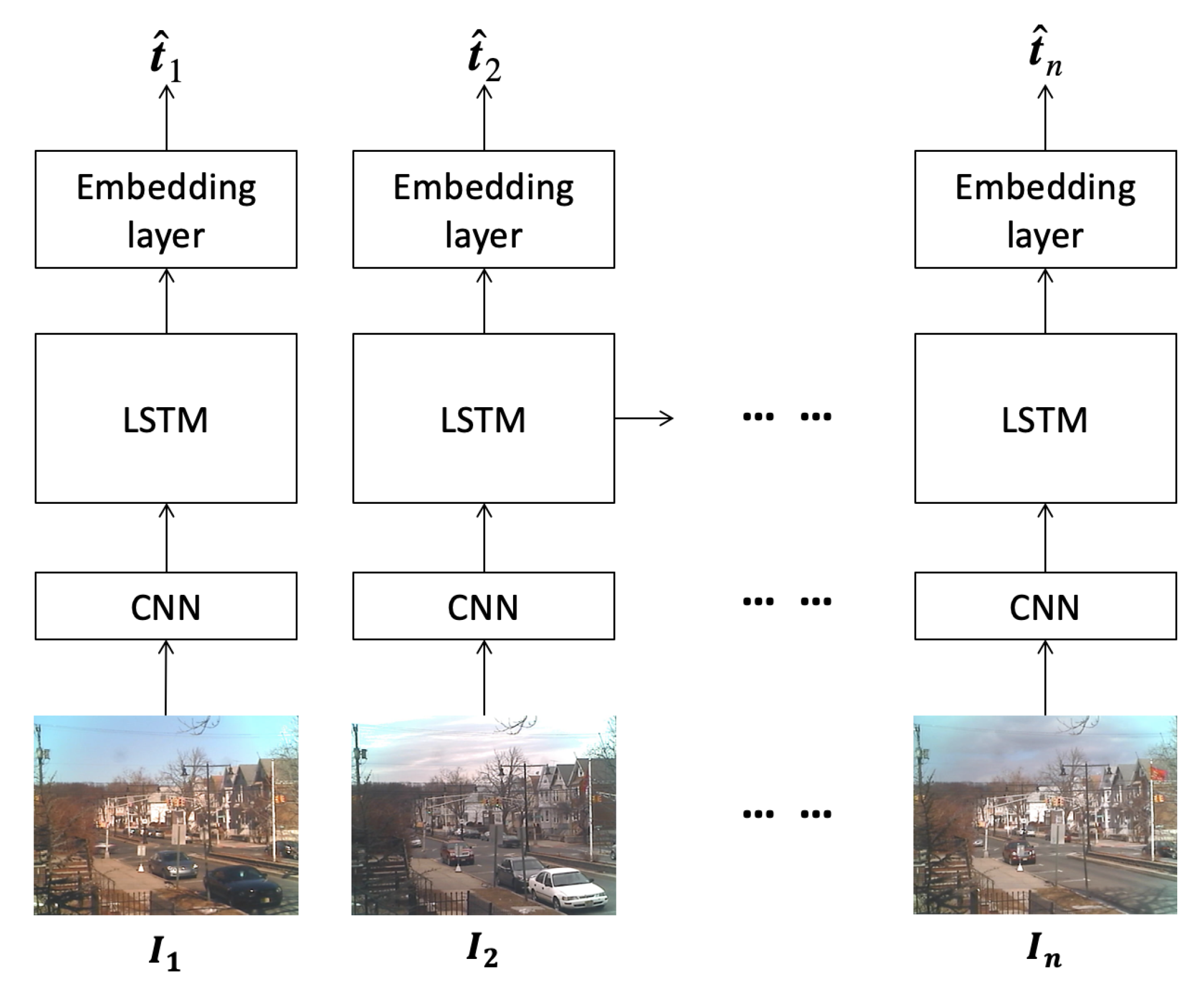
Figure 6 illustrates the network for estimating four weather properties based on multi-task learning. The CNN pre-trained for temperature prediction, as mentioned in Section 4.1, is taken as the baseline feature extractor. Given a sequence of images $I_1,I_2,...,I_n$, visual features are separately extracted from each image by the CNN. These features are then sequentially fed to the LSTM. As illustrated in Figure 6, information from $I_1$ and $I_2$ is processed and propagated, and the last LSTM outputs the predicted weather properties for the image $I_3$. Four LSTM streams are constructed to predict temperature, humidity, visibility, and wind speed, respectively.

Instead of treating four tasks separately, the network shown in Figure 6 was trained in an end-to-end manner. We respectively calculated categorical cross entropies between the predicted temperature (humidity, visibility, and wind speed) and the true temperature (humidity, visibility, and wind speed) as ${\ell }_t$, ${\ell }_h$, ${\ell }_v$, and ${\ell }_w$, respectively. They were then combined as $L={\lambda }_1{\ell }_t+{\lambda }_2{\ell }_h+{\lambda }_3{\ell }_v+{\lambda }_4{\ell }_w$, where ${\lambda }_i$s were empirically set as 0.15, 0.10, 0.90, and 0.25, respectively. Based on this loss, we adopted the Adam optimizer with learning rate 0.001 and mini batch size 128 to find the best network parameters.

6. Two-Dimensional RNN

The temporal evolution considered by previous works such as [8,10] has only day-wise predictions. That is, given day i and day $i+1$, it predicts weather properties on day $i+2$. This idea comes from that weather changes gradually on neighboring days. In this work, we further point out that weather properties usually change gradually on the same day, and we can make hour-wise predictions.

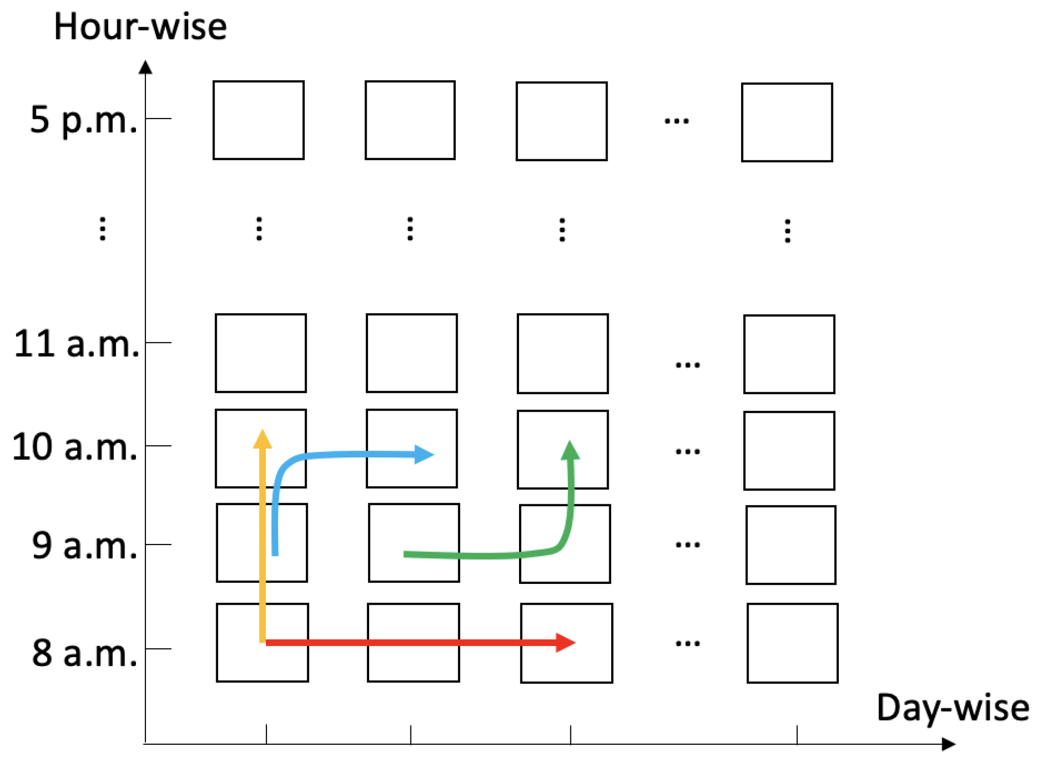
Figure 7 illustrates the idea of predicting weather properties at different temporal scales. The red arrow indicates the common day-wise perspective, and the yellow arrow indicates the hour-wise perspective, which has not been proposed or implemented before. Furthermore, with the designed 2D RNN, we would provide more flexible predictions, such as the ones shown as the green arrow and the blue arrow. As shown by the green arrow, given the images captured at 9 a.m. on day i and day $i+1$, we can predict weather properties of the image captured at 10 a.m. on day $i+1$. On the other hand, given the images captured at 9 a.m. and 10 a.m. on day $i-1$, we can predict weather properties of the image captured at 10 a.m. on day i (the blue arrow).

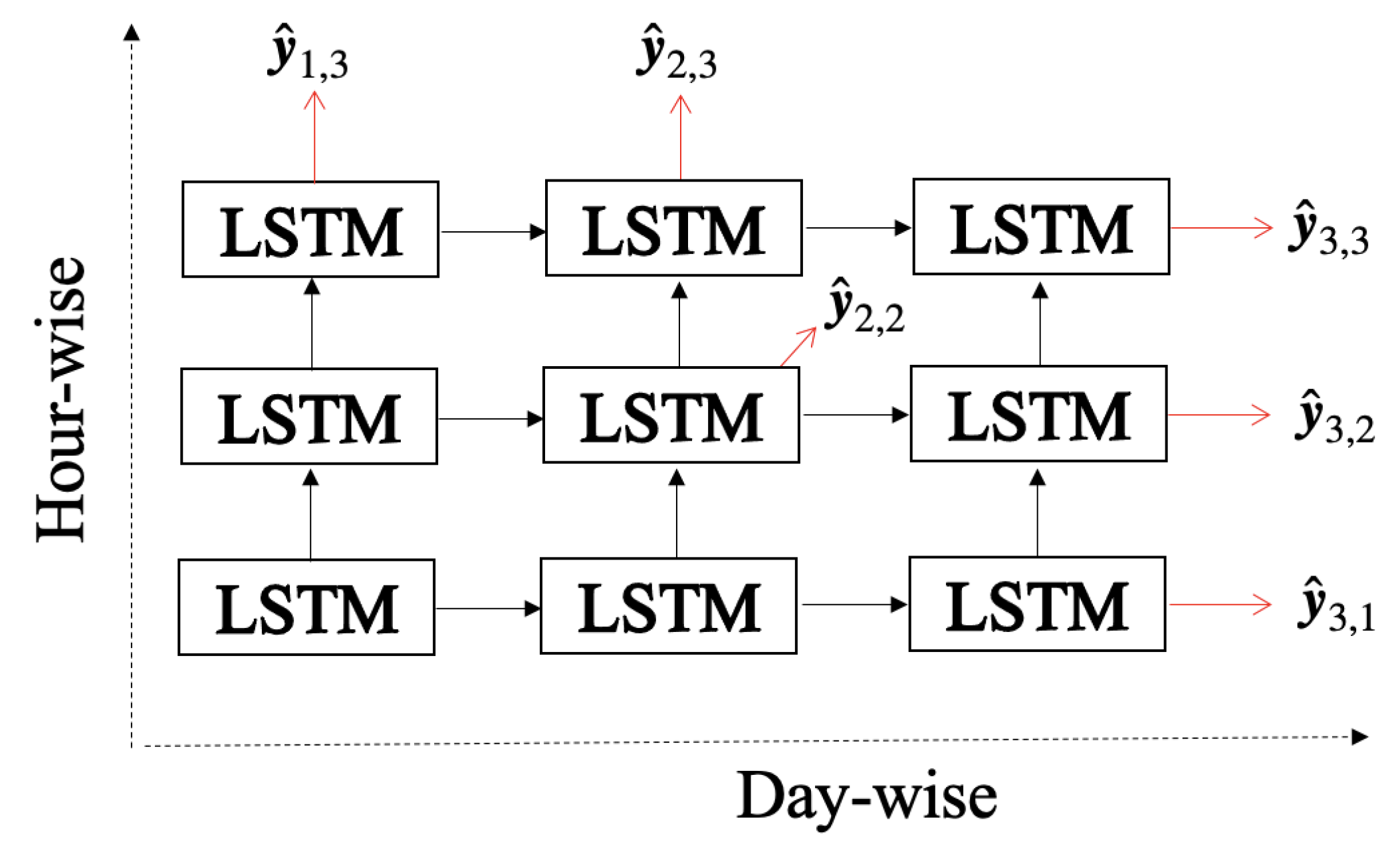
Figure 8 shows the architecture of the proposed two-dimensional RNN, where we take sequences of three images captured at three consecutive time instants as the example. The black arrows in this figure denote information propagation, and the red arrows denote the estimation outputs. Let $I_{i,j}$ denote the image captured at hour j on day i. For day-wise prediction, given the image sequence of $I_{i,j}$, $I_{i+1,j}$, and $I_{i+2,j}$ captured on days i, $i+1$, and $i+2$, the model predicts the weather properties of $I_{i+2,j}$ as ${\widehat{\mathit{y}}}_{i+2,j}$. For hour-wise prediction, given the image sequence of $I_{i,j}$, $I_{i,j+1}$, and $I_{i,j+2}$ captured at hours j, $j+1$, and $j+2$, the model predicts the weather properties of $I_{i,j+2}$ as ${\widehat{\mathit{y}}}_{i,j+2}$. We also propose that day-wise and hour-wise prediction can be mixed together. Given the image sequence of $I_{i,j}$, $I_{i+1,j}$, and $I_{i+1,j+1}$, the model predicts the weather properties of $I_{i+1,j+1}$ as ${\widehat{\mathit{y}}}_{i+1,j+1}$. Notice that, given the image sequence of $I_{i,j}$, $I_{i,j+1}$, and $I_{i+1,j+1}$, the model can also predict the weather properties of $I_{i+1,j+1}$ as ${\widehat{\mathit{y}}}_{i+1,j+1}$. For example, ${\widehat{\mathit{y}}}_{2,2}$ can be predicted by giving the image sequence $I_{1,1}$, $I_{1,2}$, and $I_{2,2}$, or by giving the image sequence $I_{1,1}$, $I_{2,1}$, and $I_{2,2}$. Overall, this model can be trained and tested based on horizontal (day-wise) sequences, vertical (hour-wise) sequences, and L-shaped (mixed) sequences.

Notice that Figure 8 is a simplified representation, where the predicted vectors ${\widehat{\mathit{y}}}_{i,j}$s are shown. In fact, with multi-task learning, we jointly predict temperature, humidity, visibility, and wind speed, and we should denote different types of estimation results as ${\widehat{\mathit{y}}}_{i,j}^{\left(t\right)}$s, ${\widehat{\mathit{y}}}_{i,j}^{\left(h\right)}$s, ${\widehat{\mathit{y}}}_{i,j}^{\left(v\right)}$s, and ${\widehat{\mathit{y}}}_{i,j}^{\left(w\right)}$s, respectively. To simplify notation, we take temperature prediction as the main instance, and just denote ground truth and the corresponding prediction result as ${\mathit{y}}_{i,j}$ and ${\widehat{\mathit{y}}}_{i,j}$, respectively. Please also notice that the numbers of LSTM layers and input/output channels are the same as those mentioned in Section 4.2. The major difference between the model in Section 4.2 and here is the perspective of the training sequences, as described below.

To train this model, we randomly selected horizontal sequences, vertical sequences, and L-shaped sequences from the training data. According to our previous work [10], the length of each image sequence (the number of images) was set as 3, as illustrated in Figure 8. The loss for each prediction is measured by categorical cross entropy. Therefore, taking temperature prediction as the main instance, the loss considering three types of sequences is:

$$L_t=\sum _{N_{1,3}}{\ell }_{1,3}+\sum _{N_{2,3}}{\ell }_{2,3}+\sum _{N_{3,3}}{\ell }_{3,3}+\sum _{N_{3,1}}{\ell }_{3,1}+\sum _{N_{3,2}}{\ell }_{3,2}+\sum _{N_{2,2}}{\ell }_{2,2},$$

(2)

where ${\ell }_{i,j}$ is the categorical cross entropy between the ground truth ${\mathit{y}}_{i,j}$ and the predicted value ${\widehat{\mathit{y}}}_{i,j}$, and $N_{i,j}$ is the number of sequences used in each specific case for training.

Overall, the losses derived from four different weather properties are integrated as $L=L_t+L_h+L_v+L_w$, where $L_h$, $L_v$, and $L_w$ are losses calculated from humidity prediction, visibility prediction, and wind speed prediction, respectively. Similarly to the training settings mentioned in Section 5, based on this loss, we adopted the Adam optimizer with learning rate 0.001 and mini batch size 128 to find the best network parameters.

7. Evaluation

7.1. Experimental Settings

To train the CNN for feature extraction as mentioned in Section 4.1, and the proposed 2D RNN model mentioned in Section 6, 90% of the images in each scene of the Glasner-Exp dataset were taken as the training pool, and the remaining 10% were taken as the testing pool. Based on the training data, we constructed a CNN consisting of six convolutional layers, followed by twp fully-connected layers.

Table 1. Detailed configurations of the convolutional neural network. Read from left to right, top to bottom.

Conv2D (32, 3)	Conv2D (32, 3) MPooling2D (2, 2)	Conv2D (64, 3)	Conv2D (64, 3) MPooling2D (2, 2) Dropout (0.25)	Conv2D (128, 3)	Conv2D (128, 3) MPooling2D (2, 2) Dropout (0.25)
Flatten	Dense (512) Dropout (0.5)	Dense (70) Softmax

shows detailed configurations of the CNN architecture. The term Conv2D(32, 3) denotes that the convolutional kernel is $3\times 3$, and the number of output channels is 32. This CNN’s output is a 70D vector indicating the probabilities of different temperatures (i.e., classes). To train the model, the activation function of each layer is ReLU, the loss function is cross entropy, the optimization algorithm is Adam, and learning rate is 0.001. This CNN was first trained to do temperature prediction specifically, and was the base model for feature extraction. When it was used in the multi-task learning, as illustrated in Figure 6, parameters of this CNN were fine-tuned according to the given training data and loss function.

To train the proposed 2D RNN model, from the training pool, we enumerated all image sequences consisting of three temporally consecutive images as the training data; i.e., these sequences could be day-wise, hour-wise, or L-shaped. A day-wise sequence could contain images $I_{i,j}$, $I_{i+1,j}$, and $I_{i+2,j}$ captured on days i, $i+1$, and $i+2$, respectively. A L-shaped sequence could contain images $I_{i,j}$, $I_{i+1,j}$, and $I_{i+1,j+1}$ captured at j o’clock on day i, at j o’clock on day $i+1$, and at $j+1$ o’clock on day $i+1$, respectively. From the training pool that consisted of images captured from 8 a.m. to 5 p.m. each day in two consecutive years, in nine different places, finally we enumerated 39,546 image sequences in total to be the training data.

Length of the image sequence. We first evaluate prediction performance when different lengths of image sequences were used for training and testing, and show the average root mean square errors (RMSEs) between the estimated values and the ground truth in

Table 2. Root mean square errors when different lengths of image sequences were used, based on the DHL-LSTM model.

	n = 2	n = 3	n = 4	n = 5	n = 6	n = 7
Temperature	2.83	2.65	2.74	2.76	2.78	2.84
Humidity	10.47	10.28	10.83	11.12	11.35	11.63
Visibility	1.42	1.42	1.44	1.47	1.53	1.61
Wind Speed	4.12	3.90	4.27	4.45	4.47	4.83

. These values were all obtained based on the full model, i.e, containing day-wise, hour-wise, and L-shaped predictions. We denote this model as DHL-LSTM in the following. As can be seen, the best estimation performance could be obtained when n was set as 3. That is, we estimated the weather properties of the day $t+2$ based on day $t+1$ and day t, if using the day-wise perspective. This result is not surprising because this setting appropriately considers information of previous days, and prevents blunt updates when too many days are considered. Therefore, we set $n=3$ in the subsequent experiments.

7.2. Single-Task Learning vs. Multi-Task Learning

Table 3. Performance comparison between single-task LSTM and multi-task LSTM for day-wise weather property prediction, in terms of RMSE. *: Our previous work [10] only focused on temperature prediction, and here we trained dedicated models for humidity, visibility, and wind speed prediction.

	Temperature	Humidity	Visibility	Wind Speed
Freq. Decom. [8]	4.47	–	–	–
LSTM (single task, four separate models) [10]	2.80	11.60 *	1.44 *	4.35 *
LSTM (multi-task, one unified model)	2.90	10.45	1.41	3.89

shows a performance comparison between the single-task LSTM [10] and the recently-proposed multi-task LSTM for day-wise weather property prediction, in terms of RMSE. For the row of single-task LSTM, we separately implemented four single-task LSTMs to predict four properties. Our previous work [10] only focused on temperature prediction, and here we trained dedicated models for humidity, visibility, and wind speed prediction to obtain the values with asterisks. As can be seen, the multi-task model obtained better performance in humidity, visibility, and wind speed predictions, and yielded slightly worse performance for temperature prediction. As pointed out by [34,35], the multi-task learning approach did not always guarantee a performance improvement. Even so, overall we see very encouraging results in Table 3. Both the single-task LSTM and the multi-task LSTM significantly outperformed [8].

7.3. Performance of 2D-RNN

Table 4. Performances of different variants of the 2D-RNN models, i.e., the day-wise-only prediction model; the hour-wise-only prediction model; the day-wise plus hour-wise prediction model; and the one containing day-wise, hour-wise, and L-shaped predictions (denoted as DHL-LSTM).

	Temperature	Humidity	Visibility	Wind Speed
Day-wise LSTM	2.90	10.45	1.41	3.89
Hour-wise LSTM	3.10	11.33	1.42	4.01
Day-wise + Hour-wise LSTM	2.78	10.33	1.41	3.89
DHL-LSTM	2.65	10.28	1.42	3.90

shows the performance variations of different 2D-RNN models, i.e., the day-wise-only prediction model; the hour-wise-only prediction model; the day-wise plus hour-wise prediction model; and the one containing day-wise, hour-wise, and L-shaped predictions. By comparing the third row with the first two rows, we can see that temperature prediction and humidity prediction are clearly improved by combining day-wise and hour-wise predictions into a single model. In this approach, a single model is trained both based on day-wise training sequences and hour-wise training sequences. Conceptually the number of training data increases, and this may be one of the reasons for the performance improvement. By comparing DHL-LSTM with the third row, clearly if we further consider L-shaped sequences, temperature prediction and humidity prediction are further improved.

Table 5. RMSEs of temperature prediction for nine different scenes, based on the single-task day-wise model, the multi-task day-wise model, the multi-task hour-wise model, the multi-task day-wise plus hour-wise model, and the DHL-LSTM model.

	(a)	(b)	(c)	(d)	(e)	(f)	(g)	(h)	(i)	Avg.
(single) Day-wise LSTM	2.23	2.28	2.68	1.78	2.75	2.32	3.16	3.51	4.47	2.80
(multi) Day-wise LSTM	2.51	2.87	2.62	3.32	3.74	2.23	2.96	2.84	3.53	2.90
(multi) Hour-wise LSTM	3.01	2.41	2.31	3.03	3.02	3.04	4.10	3.36	1.16	3.10
(multi) Day-wise + Hour-wise LSTM	2.52	2.62	2.27	2.09	2.58	1.73	3.90	3.63	3.57	2.78
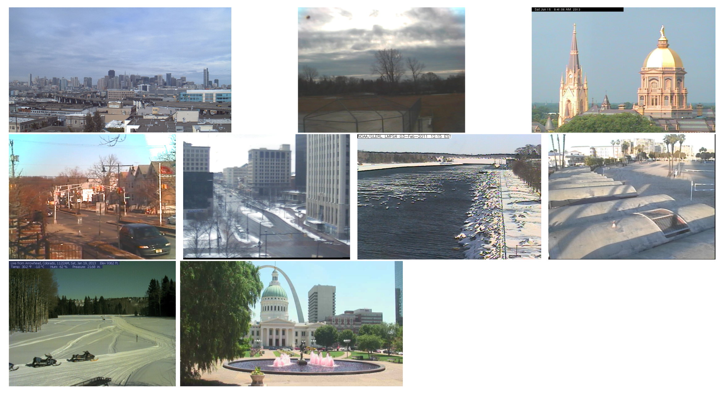
(multi) DHL-LSTM	2.46	2.60	2.32	1.73	2.76	2.18	3.01	3.51	3.27	2.65

shows detailed the performance of temperature prediction for the nine evaluated scenes. The scenes (a) to (i) correspond to the subfigures shown in Figure 2, from left to right, top to bottom. Two observations can be made. First, on average the proposed DHL-LSTM achieved the best performance. Second, performance varied for different scenes. For different scenes, sometimes the day-wise LSTM performed better, and sometimes the hour-wise LSTM performed better. This shows complex changes of weather conditions from the day-wise perspective and the hour-wise perspective. Not single perspective guarantees easier prediction.

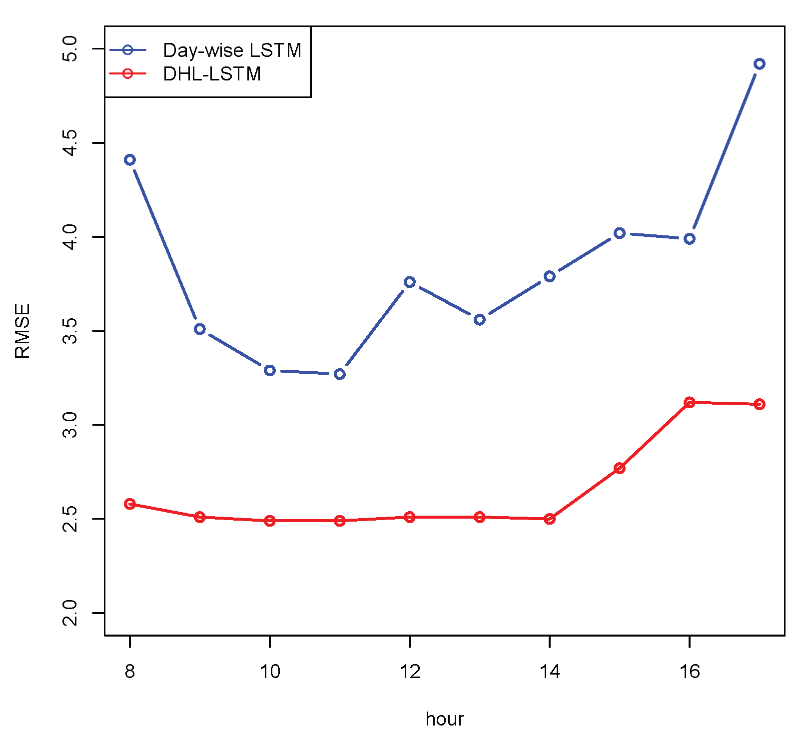
Variations of different daytime hours. During a day, the strength and direction of sunlight vary from dawn to dusk. It would be interesting to know the performance variations for different daytime hours. To show this, we used image sequences at hours h as the testing data, and the remaining for training. The hours h were 8 a.m. to 5 p.m.

Figure 9 shows variations of average RMSEs of temperature prediction for image sequences captured at different daytime hours, based on the day-wise LSTM [10] and the DHL-LSTM. We can clearly make two observations. First, for each model, we see there are clear performance variations for images captured at different daytime hours. The best performance was obtained for images captured at 11 p.m., which conformed to the selection of [8,9]. This may be because the sunlight is maximal around noon, and more robust visual information can be extracted. Second, the DHL-LSTM model significantly outperformed the day-wise LSTM model. For the day-wise LSTM, prediction errors at 8 a.m. and 5 p.m. are much larger than the others, whereas for the DHL-LSTM, the performance gap is relatively smaller, especially for images captured at 8 a.m.

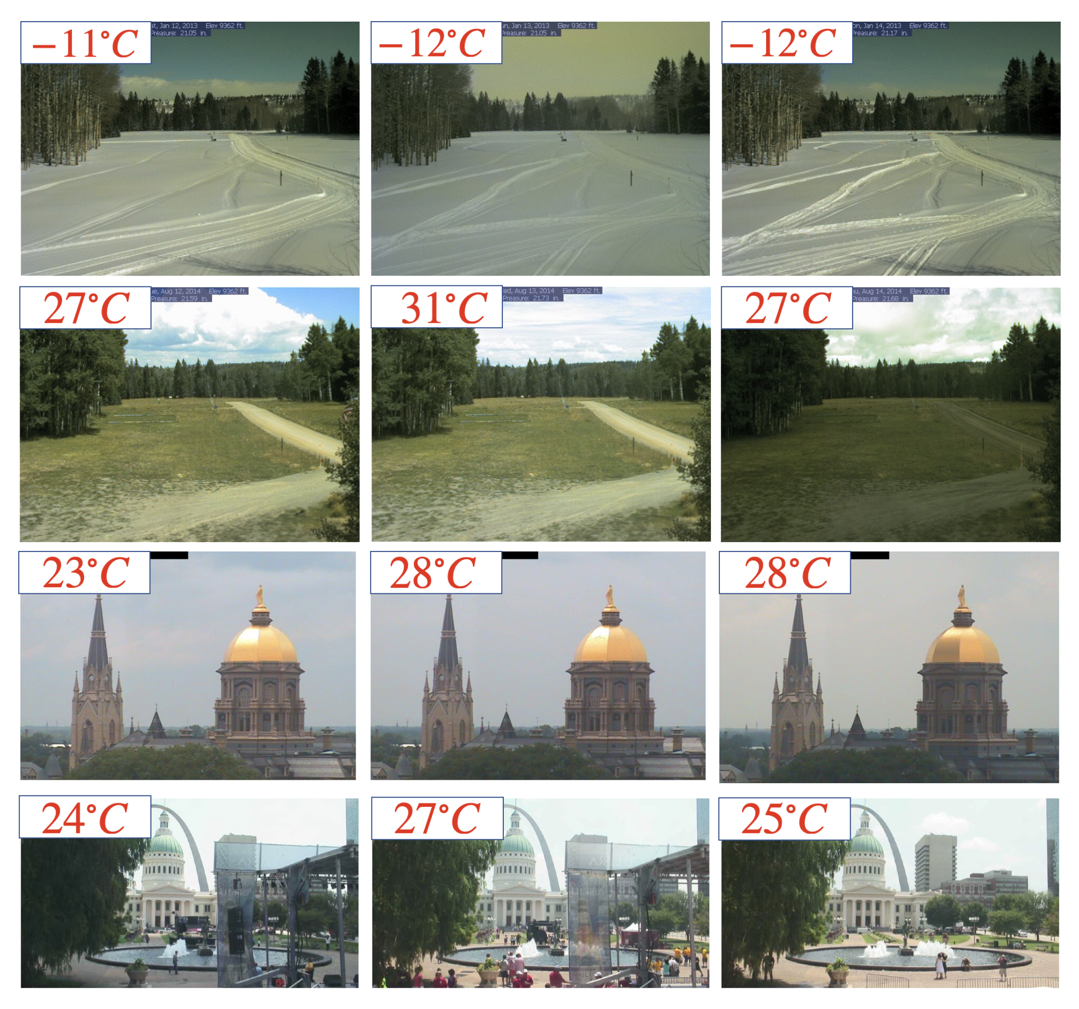
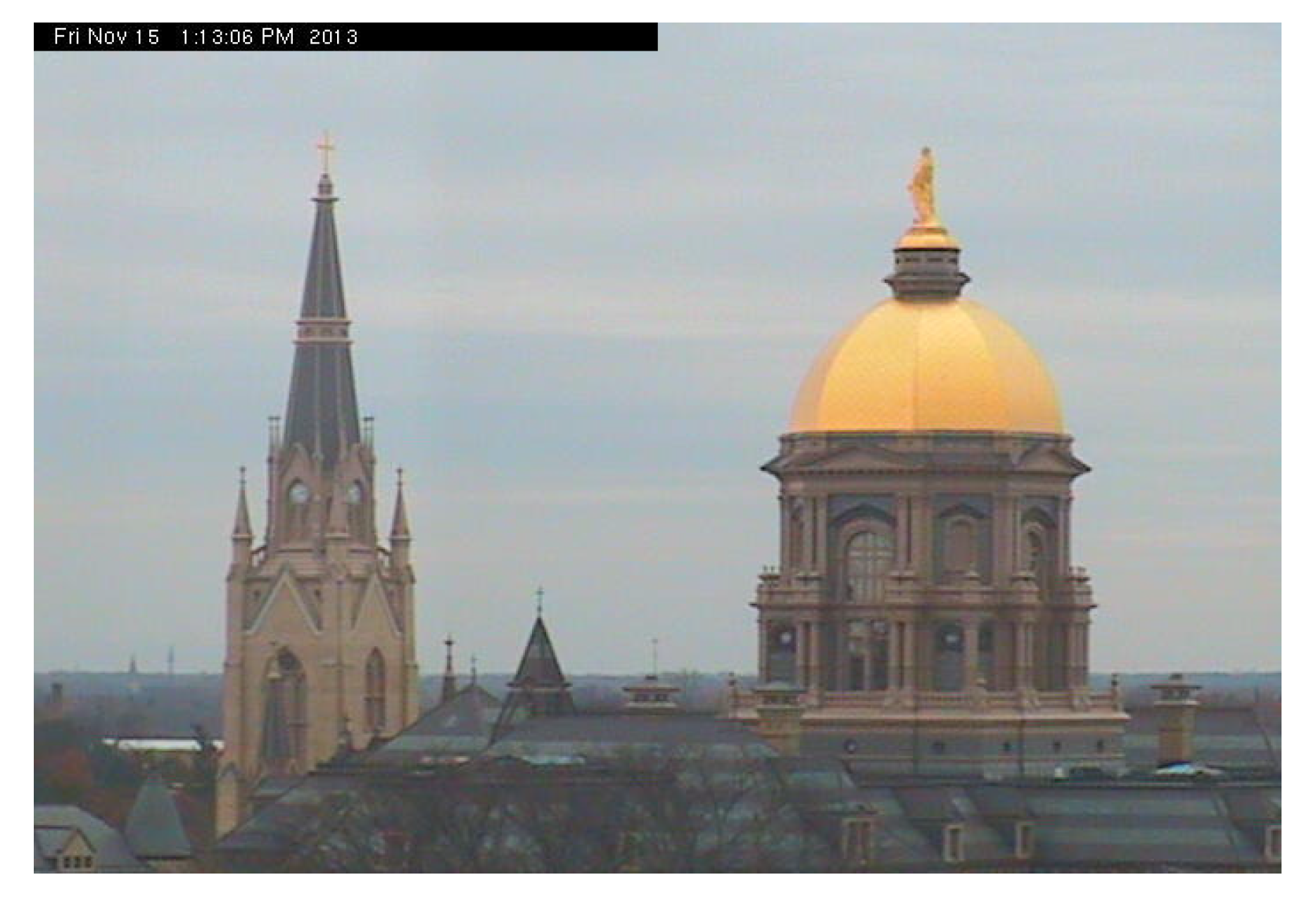
Figure 10 and Figure 11 show two sample images, and the pairs of prediction results and ground truths are shown in the captions. Figure 10 was captured at 2 p.m. on 18 May 2014, around the University of Notre Dame, Indiana, USA. Figure 11 was captured at 1 p.m. on 15 November 2013, in St. Louis, Missouri, USA. These two examples demonstrate the effectiveness of predicting weather properties from visual appearance.

8. Conclusions and Discussion

In this work, we presented deep models to estimate four weather properties of the last image in an image sequence. We jointly considered four weather properties in a unified CNN-RNN model based on the multi-task learning approach. Furthermore, we proposed considering property prediction from different temporal perspectives, i.e., day-wise, hour-wise, and the mixture of two scales. In the evaluation, we showed the effectiveness of multi-task learning and the multi-temporal-scale prediction. This is the first time that a 2D-RNN has been proposed to predict weather properties from visual appearance, and we show that state-of-the-art performance can be obtained.

In the future, we can investigate which region in a scene provides more clues in property estimation, and adopt the currently emerging attention networks to improve performance. We also believe that exploring the relationship between weather properties and vision would be interesting in a wide range of future applications.