Artifact-Free Single Image Defogging

Abstract

In this paper, we present a novel defogging technique, named CurL-Defog, with the aim of minimizing the insertion of artifacts while maintaining good contrast restoration and visibility enhancement. Many learning-based defogging approaches rely on paired data, where fog is artificially added to clear images; this usually provides good results on mildly fogged images but is not effective for difficult cases. On the other hand, the models trained with real data can produce visually impressive results, but unwanted artifacts are often present. We propose a curriculum learning strategy and an enhanced CycleGAN model to reduce the number of produced artifacts, where both synthetic and real data are used in the training procedure. We also introduce a new metric, called HArD (Hazy Artifact Detector), to numerically quantify the number of artifacts in the defogged images, thus avoiding the tedious and subjective manual inspection of the results. HArD is then combined with other defogging indicators to produce a solid metric that is not deceived by the presence of artifacts. The proposed approach compares favorably with state-of-the-art techniques on both real and synthetic datasets.

1. Introduction

Fog, mist, or haze may negatively affect the acquisition of digital photographs. Indeed, images captured under bad weather conditions may suffer from limited visibility, poor contrast, faded colors, and a loss of sharpness. This not only makes the photographs esthetically less pleasant but can greatly decrease the accuracy of computer vision tasks such as object detection, tracking, classification, and segmentation [1], which constitute the basic blocks of challenging applications such as self-driving cars. Defogging (or dehazing) is the task of removing the fog from a given image, with the aim of reconstructing the same scene as if it were taken in good (or at least better) weather conditions.

A robust haze removal technique can be useful in many circumstances, both as a pre-processing step and as a stand-alone procedure. For instance, fog is one of the main causes of road accidents; thus, a strong defogging algorithm can be extremely helpful for drivers—e.g., informing them of hazards that may be hidden behind the mist. Even self-driving cars often become extremely confused in foggy weather, due to the limited visibility and the creation of reflections and glare in the cameras [1]. Defogging can also be used as an independent operation in image enhancement tasks, with the aim of improving the visual quality of images; e.g., in photographs taken with smartphones or digital cameras.

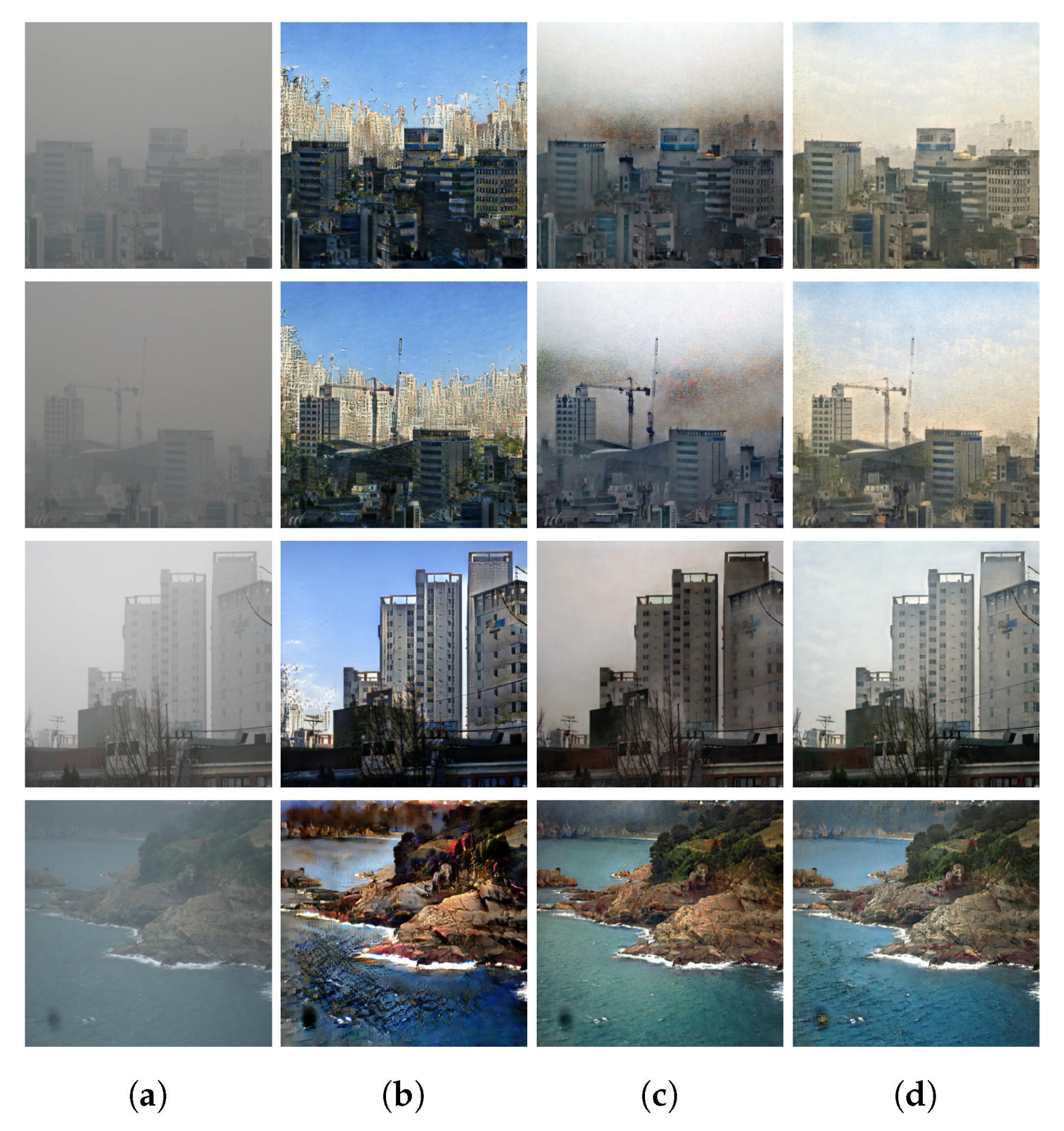
In recent years, a plethora of defogging approaches has been proposed, based on both classical neural networks [2,3,4] and generative adversarial networks [5,6,7,8]. Although these methods often outperform the preexisting state-of-the-art, they usually must be trained with paired data, namely the same scene acquired with and without fog. The impossibility to acquire perfectly paired data, alongside the increased need for big datasets, has pushed researchers to create and use synthetic data, where the fog is automatically inserted according to a physical model (see Equation (1)) [9,10,11]. Moreover, the majority of the existing defogging techniques cannot handle images with severe fog, where the visibility of the scene is highly compromised [12], limiting their practical application in real scenarios. When totally unpaired models (e.g., CycleGAN) are applied to images with severe fog, the results are visually pleasing but often affected by the presence of unwanted artifacts (see Figure 1) added by the “imagination” of the model. Such artifacts can be extremely dangerous in some applications; for example, non-existent pedestrians or obstacles added to a defogged road scene could lead an autonomous car to make incorrect decisions or behave in an unexpected manner.

In this paper, we present a novel defogging technique based on recent developments in generative adversarial networks and style transfer. To reduce the insertion of artifacts, we exploited the concept of curriculum learning [13], where a model is first trained on simpler tasks, and then the complexity of the examples is increased as the training progresses. Although this seems to be a fairly obvious strategy, curriculum learning is not easy to implement, since the curricula must be chosen in an effective manner in order to gain advantages over the traditional learning procedures [14]. We developed our curriculum learning strategy by first training our model on artificial paired data in order to compare the defogged image with the ground-truth of the real scene. This highly penalizes the insertion of artifacts, thus introducing a bias that is not destroyed in successive training phases, when the model is exposed to real unpaired data to learn more difficult transformations.

As shown in Section 5, our model is able to perform defogging more effectively on real foggy images than the majority of models trained only on artificial data. In addition, the presence of artifacts is significantly reduced with respect to the CycleGAN-based approaches. Additional tests with severe fog show that the proposed model performs well even in extreme scenarios, faithfully reconstructing the scene and not inserting unwanted artifacts in clear images.

In order to quantify the number of artifacts introduced by a defogging technique, we propose (in Section 4) a novel referenceless artifact detection method, denoted as HArD. The metric can detect, localize, and quantify the artifacts present in a defogged image without the need for a reference clear image, so it can be particularly useful to evaluate defogging on real images. We also combined the HArD metric with the indicators proposed by Hautiére et al. [15] in order to obtain an adjusted defogging metric that takes into account the amelioration of the contrast (only) outside the artifact regions.

The rest of the paper is organized as follows: Section 2 provides an overview of related work on defogging and defogging metrics. In Section 3, the proposed defogging approach is described, and in Section 4, the new metrics are illustrated. In Section 5, the experimental results are presented and widely discussed, comparing the proposed method with the current state-of-the-art. Finally, in Section 6, conclusions are drawn and future work directions are suggested.

This manuscript is an extended version of the paper Towards Artifacts-Free Image Defogging [16] presented by the same authors at the 2020 International Conference on Pattern Recognition (ICPR).

2. Related Works

2.1. Single Image Defogging

In the presence of fog or haze, the original irradiance of the scene is attenuated in proportion to the distance of the objects. This effect is combined with the scattering of atmospheric light. A simple mathematical model can be formulated as follows [17,18]:

$$I\left(x\right)=J\left(x\right)t\left(x\right)+A(1-t(x\left)\right),$$

(1)

where $I\left(x\right)$ and $J\left(x\right)$ are the hazy and clear images, respectively, A is the global atmospheric light, and $t\left(x\right)$ is the transmission map of the scene, defined as $t\left(x\right)=e^{-\beta d\left(x\right)}$, where $d\left(x\right)$ is the depth map of the scene and $\beta$ is the scattering coefficient of the atmosphere.

In theory, knowing A, $\beta$, and the depth of the scene $d\left(x\right)$, the inversion of Equation (1) can perfectly reconstruct the original clear image. However, the problem is ill-posed, and the estimation of the three parameters from single images is difficult and prone to errors. For these reasons, many defogging techniques based on the physical model directly estimate the transmission map $t\left(x\right)$ supposing A to be constant and typically equal to 1.

One of the first single image dehazing methods was proposed by Narasimhan et al. [19], and it relied on supplied information about the scene structure. An effective method was developed by Fattal [20], who used an Independent Component Analysis-based method to estimate the albedo and transmission map of a scene. He et al. [21] observed an interesting property of outdoor scenes with clear visibility: most objects have at least one color channel that is significantly darker (the pixel value for that channel is near zero) than the others. Using this property, a method based on dark channel prior was used to estimate the transmission map $t\left(x\right)$. Tarel et al. [22] proposed a technique whose complexity is linear with the number of image pixels. Their approach is based on a heuristic estimation of the atmospheric veil, which is then used to recover the haze-free image. Other classical dehazing approaches directly estimate the parameters of the aforementioned physical model from examples or exploit some statistical properties of images [23,24].

The most recent approaches are based on deep learning techniques, which are used to estimate the atmospheric light and the transmission map. An approach based on convolutional neural networks (CNN) was proposed by Ren et al. [3], where a coarse holistic transmission map is first produced using a CNN and then refined using a different fine-scale network. Cai et al. introduced a CNN called DehazeNet [2] with the goal of learning a direct mapping between foggy images and the corresponding transmission maps. None of the approaches described above consider the esthetic quality of the resulting image in the parameter estimation phase. End-to-end models, which directly estimate the clear image, began to emerge with the work by Li et al. [4].

Generative adversarial networks (GANs) [25] have proven to be effective for many image generation tasks, such as super-resolution, data augmentation, and style transfer. The application of GANs to dehazing is quite recent; most notably, the use of adversarial training for the estimation of the transmission map was proposed by Pang et al. in [5]. The use of GANs as end-to-end models to directly produce a haze-free image without estimating the transmission map was first developed by Li et al. [6]; in that model, the discriminator receives a pair of images—the hazy image and the corresponding clear image—and is trained to estimate the probability that the haze-free image is the real k age given the foggy picture.

All the CNN or GAN-based approaches reported above are trained on paired datasets of foggy and clear images. Unfortunately, these datasets are often synthetic and the quality of results may decrease if the model is tested with real photographs. CycleGAN [26], a special GAN approach based on cycle consistency loss, does not require any pairing between the two collections of data. Defogging with unpaired data was explored by Engin et al. [7]: taking inspiration from neural style transfer [27], the inception loss computed by features extracted from a VGG network [28] was used as a regularizer. Moreover, Liu et al. [8] proposed a model similar to CycleGAN used in conjunction with the physical model to apply fog to real images during the inverse mapping.

Curriculum learning was recently explored in the context of foggy scene understanding and semantic segmentation [29,30], surpassing the previous state-of-the-art in these tasks. The curriculum learning approach presented in [29] shows some similarities to our defogging approach, validating our proposal even in a different scenario. The curriculum learning approach proposed in [30] is an improvement of [29], where more than two curriculum steps are used. However, the two approaches present some differences from our proposal: in [29,30], the ground-truth data are generated with self-supervision (from the previous step model), while we do not require the ground truth when working with real foggy images. Moreover, our proposal uses generative models (GANs), while [29,30] used supervised models (CNN). Apart from these differences, we cannot compare our approach with those presented in [29,30] as they operate in a different setting; in fact, while our approach is aimed at removing the fog from images to reconstruct the same scene taken in clear weather conditions, the suggested papers focus on semantic segmentation and scene understanding.

2.2. Defogging Metrics

Assessing the quality of defogging is a particularly difficult task, especially without information about the geometry of the image such as the 3D model of the scene. As of the writing of this work, human judgment is often preferred with regard to automatic evaluation to assess the quality of defogging. However, human evaluations are subjective, onerous, tedious, and impractical for large amounts of data.

The most used automatic evaluation techniques are based on methods originally developed to assess image degradation or noise, such as structural similarity (SSIM) [31] and the peak signal-to-noise ratio (PSNR), both of which well-known in image processing (e.g., being used to estimate the quality of compression or deblurring techniques). The main problem with these metrics is that they need a reference clear image which, as stated before, is nearly impossible to obtain in a real-world scenario. In addition, SSIM and PSNR often do not correlate well with human judgment or with other referenceless metrics [9].

Recently, some referenceless metrics specifically designed for defogging have been proposed. One of these “blind” metrics was introduced by Hautière et al. [15]; it consists of three different indicators: e, $\sigma$ and $\overline{r}$. The value of e is proportional to the number of visible edges in the defogged image relative to the original foggy picture. An edge is considered visible if its local contrast is above 5%, in accordance with the CIE international lighting vocabulary [32]. The value of $\sigma$ represents the percentage of pixels that become saturated (black or white) after defogging. Finally, $\overline{r}$ denotes the geometric mean of the ratios of the gradient at visible edges; in short, it gives an indication of the amelioration of the contrast in the defogged image.

Another referenceless metric used to assess the density of fog within an image was introduced by Choi et al. [33] relying on the natural scene and fog-aware statistical features. The metric, named the Fog Aware Density Evaluator (FADE), gives an estimation of the quantity of fog in an image and seems to correlate well with human evaluation.

However, all the aforementioned metrics do not take into account the presence of artifacts in the defogged image, which is a critical issue especially when unpaired image-to-image translation models are used. Furthermore, the metrics proposed in [15] can be highly deceived by the presence of artifacts (especially the descriptors e and $\overline{r}$), since the addition of nonexistent objects can raise the number of visible edges in the defogged image. As an example, an edge in the defogged image that is located in a region where many edges are also present in the original foggy image is probably the result of a correct visibility enhancement and should be taken into consideration in the metric computation. On the other hand, a new border in the defogged image that lies in a region where no edge is visible in the associated foggy image is probably an artifact inserted by the model and should not be considered, or possibly penalized, in the metric calculation.

3. The CurL-Defog Model

Learning to translate a fogged image into a clear scene is a difficult task, especially without a reference to clear images during training. Indeed, having a reference ground truth, as in the pix2pix model [34], produces better results than a totally unpaired approach, such as the CycleGAN model [26], which inserts almost no artifacts and enhances the contrast more effectively. On the other hand, training a model only with synthetic images produces poorer results when tested with real foggy photographs, limiting its practical application in real scenarios.

In order to train a model with real images and at the same time reduce the artifacts inserted during the defogging, we propose CurL-Defog, an approach inspired by curriculum learning [13], where the model is first guided towards a desirable parameter-space region via pix2pix-like [34] training using a synthetic paired image. The model is then refined by more complex CycleGAN-like training, where real unpaired images are progressively provided. As the model’s parameters already lie in a favorable region at the beginning of the refinement stage, it is unlikely they will be greatly moved to distant configurations leading to the introduction of heavy artifacts.

3.1. The Model

The two training phases of the proposed model are not separated (e.g., first, the model is trained only with artificial images, and then only with real photographs), but there is a gradual transition from the paired training to the unpaired training. Indeed, at each epoch, the model is trained with some synthetic images and some real images. As the epochs go on, the number of artificial images is reduced while the number of real examples grows, progressively increasing the influence of unpaired training.

During the paired training (where the model is trained with artificial data), we use two different pix2pix models: one for defogging fogged images and one for adding fog to clear images. In this phase, the two submodels are trained separately. Conversely, during the unpaired training, the model can be seen as a CycleGAN-based model, where both the fogging and defogging networks are used in combination to enforce the cycle consistency loss.

Overall, CurL-Defog is composed of four networks: a generator $G_{defog}$ used for defogging, a generator $G_{fog}$ used for inserting fog, a discriminator $D_{clear}$ used to discriminate between real and defogged images, and a discriminator $D_{fog}$ used to discriminate between real and generated foggy images. The overall approach is graphically shown in Figure 2, and the training algorithm is summarized in Algorithm 1.

3.2. Networks

Generator networks: The architecture of the generator is the same for both $G_{defog}$ and $G_{fog}$. We have adopted an encoder–decoder network inspired by the work of Johnson et al. [27] due to the impressive results in neural style transfer. The networks contain three convolutional blocks in the encoding module and three convolutional blocks in the decoding module. Every convolutional block is followed by an instance normalization [35] layer and a ReLU activation layer. In the encoder, the first layer has 64 filters with a kernel size of 7 × 7 and stride of 1. The second and third layers have 128 and 256 filters, respectively, with a kernel size of 3 × 3 and stride of 2. Each layer of the decoder module has the same number of filters as its symmetric layer in the encoder module, but the convolutions have a stride of 1/2 (transposed convolution). To perform the translation, we have used nine residual blocks [36], in a similar manner to the original CycleGAN implementation. The detailed architecture of the generator is shown in

Table 1. Architecture of generator networks.

Layer	Activation Size
Input	3 × 256 × 256
32 × 7 × 7 conv, stride 1, reflective padding 3	32 × 256 × 256
64 × 3 × 3 conv, stride 2, padding 1	64 × 128 × 128
128 × 3 × 3 conv, stride 2, padding 1	128 × 64 × 64
Residual block, 128 filters	128 × 64 × 64
…	…
Residual block, 128 filters	128 × 64 × 64
64 × 3 × 3 conv, stride 1/2, padding 1	64 × 128 × 128
32 × 3 × 3 conv, stride 1/2, padding 1	32 × 256 × 256
3 × 7 × 7 conv, stride 1, reflection padding 3	3 × 256 × 256

.

Discriminator networks: Both discriminators $D_{clear}$ and $D_{fog}$ are based on the same architecture: a 70 × 70 patchGAN [37] aimed at classifying 70 × 70 overlapping image patches as real or fake. The model contains fewer parameters than a classical image classification network and can operate on images of any size due to its fully convolutional architecture. The detailed architecture of the discriminator is shown in

Table 2. Architecture of discriminator networks.

Layer	Activation Size
Input	3 × 256 × 256
64 × 4 × 4 conv, stride 2, padding 1	64 × 128 × 128
128 × 4 × 4 conv, stride 2, padding 1	128 × 64 × 64
256 × 4 × 4 conv, stride 2, padding 1	256 × 32 × 32
512 × 4 × 4 conv, stride 1, padding 1	512 × 31 × 31
1 × 4 × 4 conv, stride 1, padding 1	1 × 30 × 30

.

Algorithm 1 CurL-Defog training algorithm. More details are provided in Section 3.3. The number of artificial and real images used in every epoch (lines 2–3) is discussed in Section 5.

1: for number of epochs do

2:     $k=$ nr. of artificial images in the current epoch

3:     $j=$ nr. of real images in the current epoch

4:     for k do                                                                                         ▷ paired training

5:         Draw a pair $(c,f)$ from the paired dataset.

6:         $\widehat{c}\leftarrow G_{defog}\left(f\right)$

7:         $\widehat{f}\leftarrow G_{fog}\left(c\right)$

8:         Calculate ${\mathcal{L}}_{pair}$ using Equation (5).

9:         Back-Propagate ${\mathcal{L}}_{pair}$

10:         Update $G_{defog},G_{fog},D_{clear}$ and $D_{fog}$.

11:     end for

12:     for j do                                                                              ▷ unpaired training

13:         Draw c from the real clear dataset.

14:         Draw f from the real foggy dataset.

15:         $\widehat{c}\leftarrow G_{defog}\left(f\right)$

16:         $\widehat{f}\leftarrow G_{fog}\left(c\right)$

17:         $f_{rec}\leftarrow G_{fog}\left(\widehat{c}\right)$

18:         $c_{rec}\leftarrow G_{defog}\left(\widehat{f}\right)$

19:         Calculate ${\mathcal{L}}_{unpair}$ using Equation (9).

20:         Back-Propagate ${\mathcal{L}}_{unpair}$

21:         Update $G_{defog},G_{fog},D_{clear}$ and $D_{fog}$.

22:     end for

23: end for

3.3. Full Objective

Paired training: During paired training, the losses of the model are based on the original pix2pix implementation [34]. As in [26], we used a squared loss instead of the cross-entropy for the adversarial loss as it improves the stability of the training and produces better results. The adversarial loss for defogging is defined as follows:

$${\mathcal{L}}_{adv}^{defog}={(D_{clear}\left(c\right)-1)}^2+{\left(D_{clear}\left(G_{defog}\left(f\right)\right)\right)}^2,$$

(2)

where $D_{clear}$ is the clear images discriminator, $G_{defog}$ is the defog network, f is the foggy image, and c is the clear image. Similarly, the adversarial loss of the fogging module is defined as follows:

$${\mathcal{L}}_{adv}^{fog}={(D_{fog}\left(f\right)-1)}^2+{\left(D_{fog}\left(G_{fog}\left(c\right)\right)\right)}^2.$$

(3)

As in the pix2pix model, the adversarial loss is joined with the L1 loss, calculated between the translated and the ground-truth images. The L1 loss is defined as follows:

$${\mathcal{L}}_{L1}=\parallel G_{defog}{\left(f\right)-c\parallel }_1+{\parallel G_{fog}\left(c\right)-f\parallel }_1.$$

(4)

The full objective of the paired training phase is obtained by combining the adversarial loss and the L1 loss as follows:

$${\mathcal{L}}_{pair}={\mathcal{L}}_{adv}^{defog}+{\mathcal{L}}_{adv}^{fog}+{\lambda }_{L1}{\mathcal{L}}_{L1},$$

(5)

where ${\lambda }_{L1}$ controls the relative importance of the L1 loss.

Unpaired training: during unpaired training, the model is trained with unpaired foggy and clear images, so the L1 loss cannot be used. Instead, we used the cycle consistency loss derived from the CycleGAN model [26]:

$${\mathcal{L}}_{cyc}=\parallel G_{fog}\left(G_{defog}\left(f\right)\right){-f\parallel }_1+{\parallel G_{defog}\left(G_{fog}\left(c\right)\right)-c\parallel }_1,$$

(6)

where f and c represent the foggy and clear images, respectively.

In order to make the defogging more effective and preserve details in the results, a cycle perceptual loss based on features extracted with a pretrained VGG-16 network [28] was introduced following the work of Engin et al. [7]. The cycle perceptual loss is defined as

$${\mathcal{L}}_{perc}=\parallel \varphi \left(f\right)-\varphi \left(G_{fog}\left(G_{defog}\left(f\right)\right)\right){\parallel }_2^2+{\parallel \varphi \left(c\right)-\varphi \left(G_{defog}\left(G_{fog}\left(c\right)\right)\right)\parallel }_2^2,$$

(7)

where $\varphi (·)$ represents features extracted from the second and fifth pooling layers of the VGG-16 network. Furthermore, similar to the original CycleGAN implementation [26], we also included an identity loss with the aim of preserving the original tint and color of the images. Identity loss is defined as

$${\mathcal{L}}_{idt}=\parallel G_{fog}{\left(f\right)-f\parallel }_1+{\parallel G_{defog}\left(c\right)-c\parallel }_1.$$

(8)

Finally, the overall objective of the model during the unpaired training can be expressed as

$${\mathcal{L}}_{unpair}={\mathcal{L}}_{adv}^{defog}+{\mathcal{L}}_{adv}^{fog}+{\lambda }_{cyc}{\mathcal{L}}_{cyc}+{\lambda }_{perc}{\mathcal{L}}_{perc}+{\lambda }_{idt}{\mathcal{L}}_{idt},$$

(9)

where ${\lambda }_{cyc},{\lambda }_{perc}$ and ${\lambda }_{idt}$ control the relative importance of cycle consistency loss, perceptual loss, and identity loss, respectively.

4. The HArD Artifact Detector

As discussed in Section 2, some ad-hoc metrics to assess the quality of defogging techniques have been proposed, each focusing on a different aspect such as the level of fog [33] or the amelioration of contrast [15].

However, the aforementioned metrics do not take into account the presence of artifacts in the defogged image, which is a critical issue especially when unpaired image-to-image translation models are used. For example, the metrics proposed in [15] can be deceived by the presence of artifacts, since the addition of nonexistent objects can increase the number of visible edges in the defogged image.

Here, we propose HArD (Haze Artifact Detector), a new referenceless artifact detector, to localize and quantify the amount of artifacts in a defogged image, given the corresponding foggy scene. HArD is based on the simple assumption that if a region in the original foggy image does not present any edge (i.e., it is a region of constant intensity), the defogging method should not introduce any object in that region, since there is no information to exploit to reconstruct the scene. In other words, if in the original foggy picture, no object can be found in a region, that region should also not contain any object in the defogged picture. The pseudocode of the HArD artifact detector is illustrated in Algorithm 2.

Algorithm 2 HArD metric calculation.

Require: $f=$ original foggy image in range (0,1)

Require: $d=$ automatically defogged image in range (0,1)

1: procedure HArD(f, d)

2:     $f^{\prime }\leftarrow$Prewitt($f_{gray}$)

3:     $d^{\prime }\leftarrow$Prewitt($d_{gray}$)

4:     $f_{smooth}^{\prime }\leftarrow$GaussianFilter($f^{\prime }$)                                                                  ▷ $\sigma =20$

5:     $d_{smooth}^{\prime }\leftarrow$GaussianFilter($d^{\prime }$)                                                                  ▷ $\sigma =20$

6:     $f_{scaled}^{\prime }\leftarrow$Normalize($f_{smooth}^{\prime }$)

7:     $f_{sat}^{\prime }\leftarrow tanh({\nu }_{fog}·f_{scaled}^{\prime })$                                                              ▷ ${\nu }_{fog}=7.5$

8:     $d_{scaled}^{\prime }\leftarrow$Normalize($d_{smooth}^{\prime }$)

9:     $d_{sat}^{\prime }\leftarrow tanh({\nu }_{defog}·d_{scaled}^{\prime })$                                                       ▷ ${\nu }_{defog}=1.5$

10:     $diff\leftarrow min(0,d_{scaled}^{\prime }-f_{sat}^{\prime })$

11:     return Mean($diff$)

12: end procedure

13:

14: procedure Normalize(im)

15:     return ($im-dat{a}_{min}/(dat{a}_{max}-dat{a}_{min})$▷$dat{a}_{min}$ and $dat{a}_{max}$ are the minimum and maximum value of the smoothed images computed offline on a reference dataset.

16: end procedure

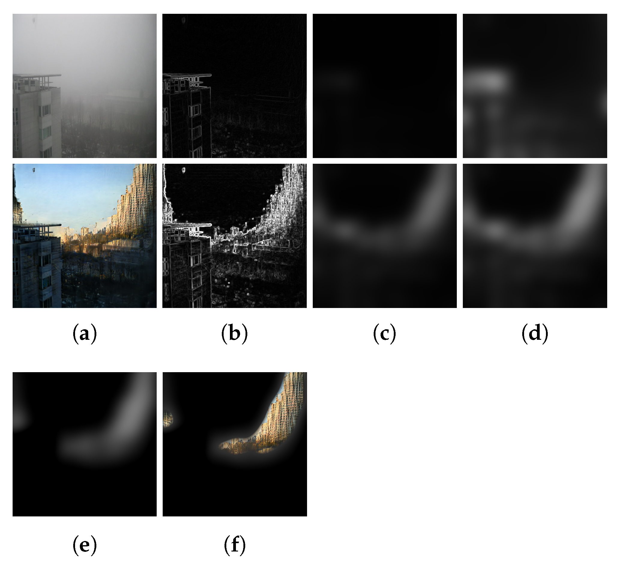
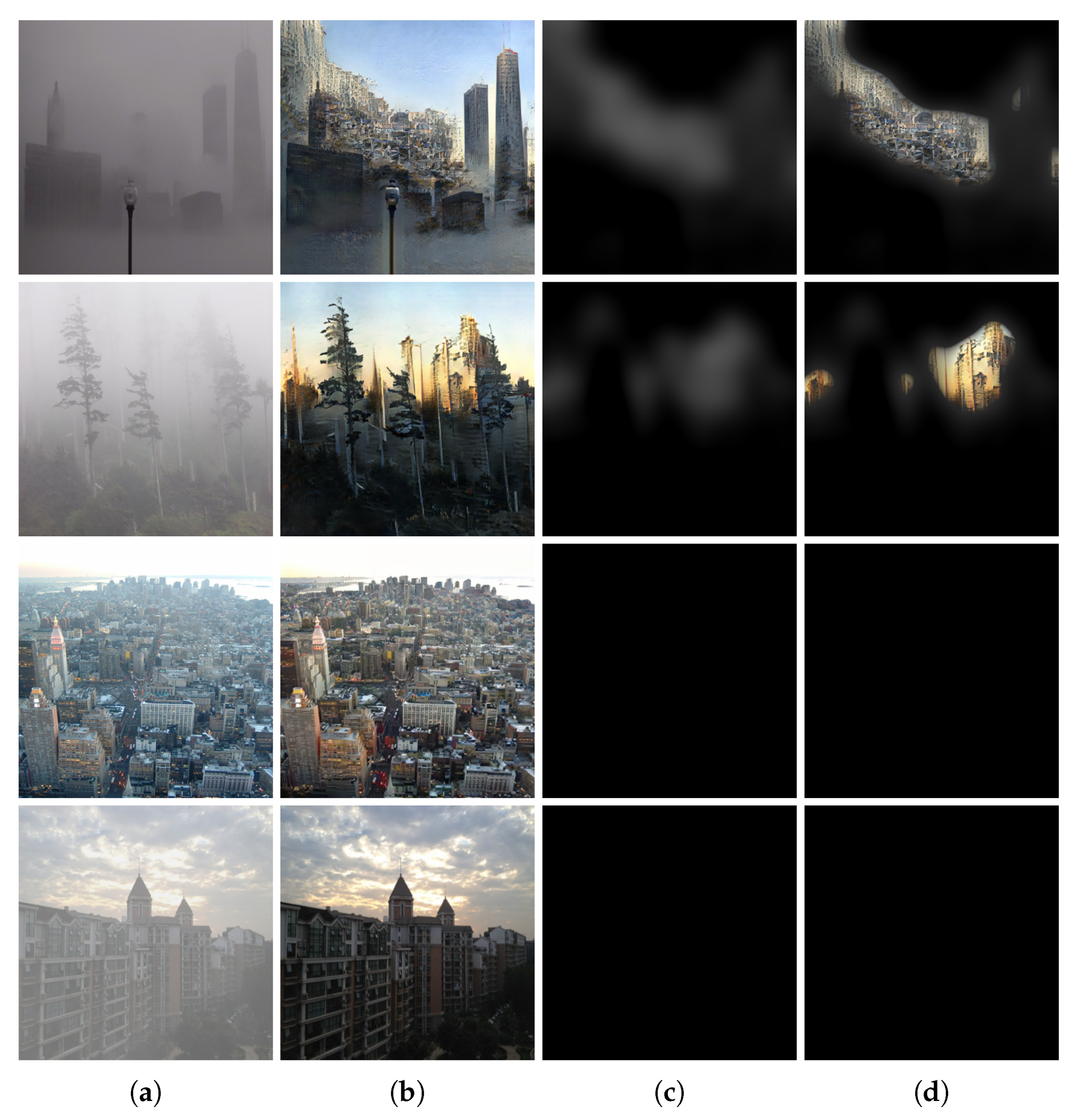
HArD can be implemented through a sequence of image processing steps (see Algorithm 2): first, a map of edges concentration in the foggy and defogged images is estimated by computing the module of the gradient using the Prewitt operator. After the edges are found, they are smoothed by convolution with a Gaussian filter. The dimension of the sigma of the Gaussian filter is set to the square root of the image dimension in order to obtain a coarse map of the gradients. The maps are then normalized in the range [0,1] using the maximum and minimum values of smoothed images extracted from a reference dataset. This is required as fog images show an especially wide range of gradient magnitudes (due to the different levels of fog). Then, both the maps are saturated by multiplying them by two constants and applying the hyperbolic tangent function; this step is performed with the aim of making the edge regions in the two images comparable, even if the defogged image is usually much more contrasted. Finally, the artifact regions in the defogged images are determined by subtracting the saturated foggy edge density map from the defogged edge density map. The obtained difference map has high values in regions denoted by the presence of edges in the defogged image but not in the fogged image. An example is shown in Figure 3. To numerically quantify the amount of artifacts inserted, we propose to use the mean of the resulting map as the indicator. This allows HArD to be receptive to both the quantity and the magnitude of artifacts. A defogging method that produces few but very clear artifacts should be penalized in the same manner as different methods that produce less evident artifacts but spread them across all the resulting images. However, the mean is often very small, so we multiply it by 100. More examples of the artifacts regions detected by our metrics are shown in Figure 4.

It is worth noting that classical image gradients based on 3 × 3 masks (such as the Prewitt operator) are theoretically poorly justified. However, in our HArD detector, the Prewitt operator is used only for coarse edge detection, and alternative gradient or contrast operators can be used in this step, such as the Michelson contrast [38] or the LIP additive contrast [39], which correlate well with the human visual system. Finally, we would like to remark that the HArD artifact detector should not be used in isolation to evaluate the quality of the defogging, since it only quantifies the presence of artifacts in the results. We recommend the use of HArD in conjunction with more traditional defogging metrics in order to give broader insights about the quality of the analyzed defogging method. A possible use of HArD in conjunction with a defogging metric is detailed in below.

The HArD + e and HArD + $\overline{r}$ Metrics

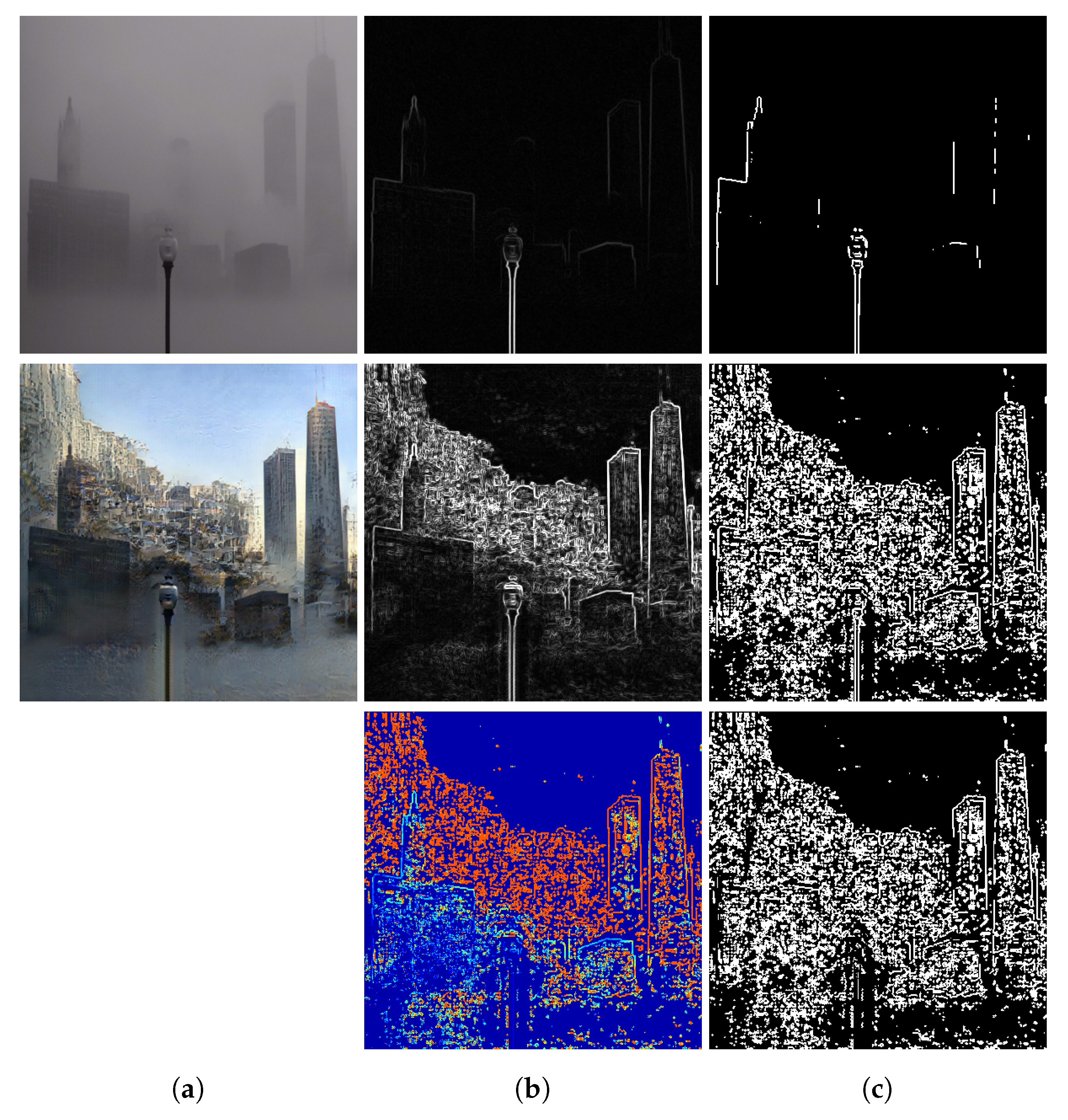
As discussed in Section 4, most of the existing metrics used to assess the quality of defogging were not conceived to deal with the insertion of artifacts, which are typical of recent deep-learning-based generative models. On the other hand, carefully designed metrics, such as the one proposed by Hautiére et al. [15], provide very useful information about quality enhancement. As examined in Section 2, the metric is composed of three indicators—e, $\sigma$ and $\overline{r}$—but here we focus only on e and $\overline{r}$. Both the indicators are based on the number of visible edges in the foggy and defogged images. The more edges are present after the defogging, the higher the value of the indicators will be. In particular, e is calculated as the number of edge pixels in the defogged image that are not detectable in the foggy image but visible after the defogging divided by the number of edge pixels that belong to visible edges in the foggy image. It is simple to understand that having a large number of artifacts, with associated edges, in the defogged image can easily increase e in an unfair manner. Similar considerations apply to $\overline{r}$. In fact, $\overline{r}$ represents the geometric mean of the ratio of the gradients of the defogged and foggy images, calculated in every visible edge pixel. Even in this case, it is simple to understand how the indicator can be deceived as an artifact could produce a visible edge in the defogged image that does not exist in the real foggy picture. Calculating the ratio of the gradients at those particular locations may produce very high values, or even infinite values if there are no edges at all in the examined location of the foggy image. An example of how the indicators e and $\overline{r}$ could be deceived by artifacts is shown in Figure 5.

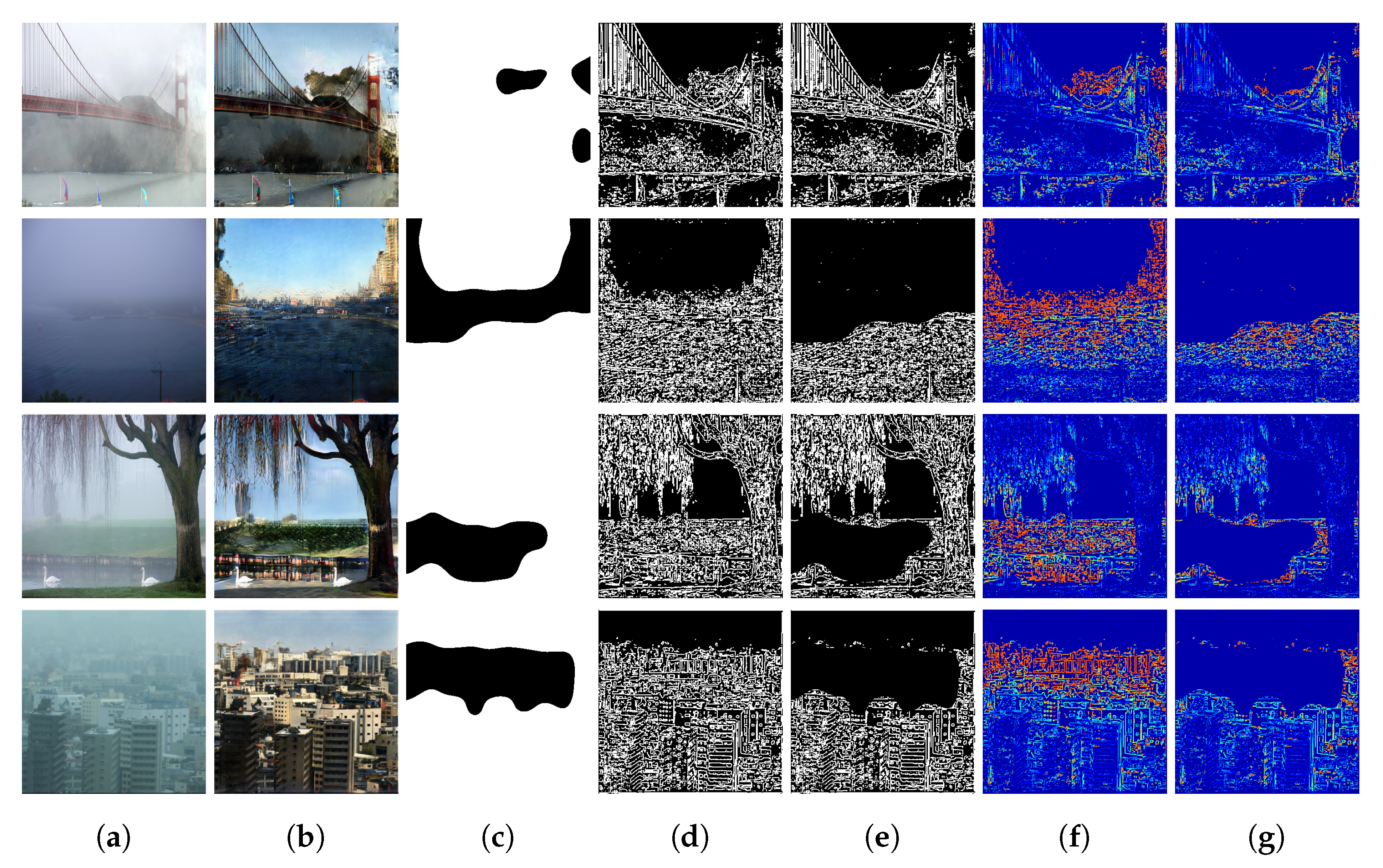
To make the indicators proposed by Hautiére et al. [15] robust against artifacts, we propose to mask out the visible edges that lie in regions where the HArD detector finds artifacts. This simple procedure allows the calculation of the effective contrast enhancement of the analyzed defogging approach, discarding regions where artifacts may deceive the metrics. To this end, we binarized (by global thresholding) the continuous artifact maps returned by HArD. After some tests, we chose a threshold equal to 0.1, since this is high enough to tolerate the noise present on the map but still includes all the regions with artifacts in the resulting binarized mask.

The mask is then inverted and multiplied by the map of the visible edges of the defogged image. Finally, since only pixels outside the mask are taken into consideration, the values need to be normalized by multiplying them by the ratio between the number of pixels in the image and the number of pixels not belonging to the mask. The indicators obtained in this manner are named HArD + e and HArD + $\overline{r}$. A visual demonstration of the benefit of the combination of the two metrics is shown in Figure 6, and detailed numerical data are reported in

Table 3. Values for the indicators e and $\overline{r}$ [15] and the proposed HArD + e and HArD + $\overline{r}$ metrics for the images in Figure 6.

	e	HArD + e	$\overline{\mathit{r}}$	HArD + $\overline{\mathit{r}}$
Row 1	1.231	1.129	3.283	3.082
Row 2	9.174	7.425	6.980	5.120
Row 3	0.475	0.160	2.925	2.538
Row 4	1.477	0.880	6.653	4.106

.

5. Experimental Results

In this section, the proposed CurL-Defog approach is evaluated and compared with some state-of-the-art defogging methods. We report experiments both on artificial and real foggy images, with a particular emphasis on scenes with severe fog and reduced visibility.

5.1. Training Details

The images used in all the experiments have different sizes and resolutions. Thus, during training, all the images were scaled to 286 × 286 pixels using bicubic interpolation, and then a random crop of size 256 × 256 was taken and used as an input to the networks. This last pre-processing step served as a sort of data augmentation procedure since the datasets were not composed of a high number of images. To reduce oscillations when the model was trained in the unpaired training phase, we followed the strategy proposed by Shrivastava et al. [40], where the discriminators were updated by using a history of generated images instead of those produced by the generators. We kept an image pool of the last 50 generated images and randomly chose one of them to train the discriminators. For all the experiments, we maintained the same parameters:

$${\lambda }_{L1}=100{\lambda }_{cyc}=10{\lambda }_{perc}=0.1{\lambda }_{idt}=0.5·{\lambda }_{cyc}.$$

These parameter values were empirically selected without performing any systematic grid search; thus, we believe that accuracy can be further improved if hyperparameter fine-tuning is adopted. In all the experiments, the CurL-Defog model was trained for 200 epochs. The learning rate was initially set to $2\times {10}^{-4}$, kept unaltered for the first 100 epochs, and then linearly reduced to zero in the last 100 epochs.

5.2. Curriculum Learning Strategy

The precise curriculum learning strategy is not explicitly specified in the CurL-Defog algorithm, so many different approaches could be used. The simplest strategy, denoted as linear, works as follows: during the first epoch, the model is trained only with artificial data; as the epochs progress, the number of artificial images is linearly decreased, reaching zero at the last epoch; conversely, the number of real images is linearly increased, reaching the maximum in the last epoch. Thus, in every epoch, a different number of real and synthetic images is present, and our model is trained both in a paired and in an unpaired manner in each training iteration.

We experimented with other possible strategies; in particular, the other two approaches denominated as linear–saturate and step. In the step strategy, only artificial images were used for the first half of the epochs, and only real images for the remaining half. This is similar to classical curriculum learning strategies, where there is no mixing of the data between different curricula. The linear–saturate strategy is similar to the linear strategy, but the model was trained only with real data for the last k epochs. These two alternatives did not show any advantage over the simple linear strategy, which also produced a smaller number of artifacts; thus, the linear strategy was used for all the following experiments.

5.3. Experiments on Synthetic Data

To assess the performance of CurL-Defog on synthetic data, we used the classical SSIM and PSNR metrics. In fact, even if improved versions of such metrics have been introduced (such as MS-SSIM [41]), SSIM and PSNR have been used by most of the methods we considered for comparison, and they remain two of the most used metrics in the defogging literature. In the synthetic data experiment, we compared our approach with both classical methods [21,23,24] and machine learning techniques [2,3,4]. We also included the pix2pix model [34] as a baseline for GAN-based methods, as the inclusion of paired data was exactly the scenario in which pix2pix was introduced. The datasets used in this experiment were as follows:

• Synthetic paired dataset (training): The Outdoor Training Set (OTS), included in the RESIDE dataset [9]. The dataset is composed of 2061 clear images where, for each image, 35 different levels of haze are applied (varying the parameters A and $\beta$ of Equation (1)), for a total of 72,135 training images. This dataset was used to train all the compared learning-based approaches;
• Real unpaired dataset (training): LIVE image defogging [42], composed of 500 clear and 500 foggy real photographs. The major issues with the LIVE dataset are the low number of images and the marked difference between foggy and clear photographs. Thus, we substituted the 500 clear images with 2.651 clear photographs taken from the RESIDE dataset [9] (with no intersection between the images used for the synthetic dataset experiments). The clear images were manually selected in order to include only daytime photographs with clear skies and good lighting. This was used for CurL-Defog training;
• Test dataset: The Hybrid Subjective Testing Set (HSTS), included in the RESIDE dataset and used as a test dataset in the benchmark by Li et al. [9].

The results are reported in

Table 4. Average SSIM and PSNR scores of the dehazing on the HSTS testing set (synthetic images). ↑ indicates that a higher value is better.

	DCP [21]	CAP [23]	NLD [24]	DehazeNet [2]	MSCNN [3]	AOD-Net [4]	Pix2Pix [34]	CurL-Defog
PSNR (↑)	14.84	21.53	18.92	24.48	18.64	20.55	24.22	24.83
SSIM (↑)	0.7609	0.8727	0.7411	0.9183	0.8168	0.8973	0.8991	0.9037

. It is worth noting that our approach is in line with state-of-the-art models, reaching the first score for PSNR and the second for SSIM, even if CurL-Defog was not designed to rival existing state-of-the-art approaches on synthetic data. A visual comparison between the different methods is shown in Figure 7.

5.4. Experiments on Real Images

Real foggy images are intrinsically unpaired, so SSIM and PSNR cannot be used to assess the effectiveness of defogging. Therefore, the referenceless metric proposed by Hautière et al. [15] was used to evaluate the results alongside the proposed HArD metric to detect the presence of artifacts and the adjusted indicators HArD + e and HArD + $\overline{r}$. CurL-Defog was here compared against the Cycle–Dehaze unsupervised approach [7], and the pix2pix model [34] was used as a baseline. The datasets used in this experiment were as follows:

• Synthetic paired dataset (training): The Outdoor Training Set (OTS), included in the RESIDE dataset [9], which was used to train pix2pix and CurL-Defog;
• Real unpaired dataset (training): LIVE image defogging [42], enhanced with more images as described in the experiment on synthetic data. Used for Cycle-Dehaze and CurL-Defog training;
• Test dataset: Test set of the LIVE image defogging dataset (100 images) [42].

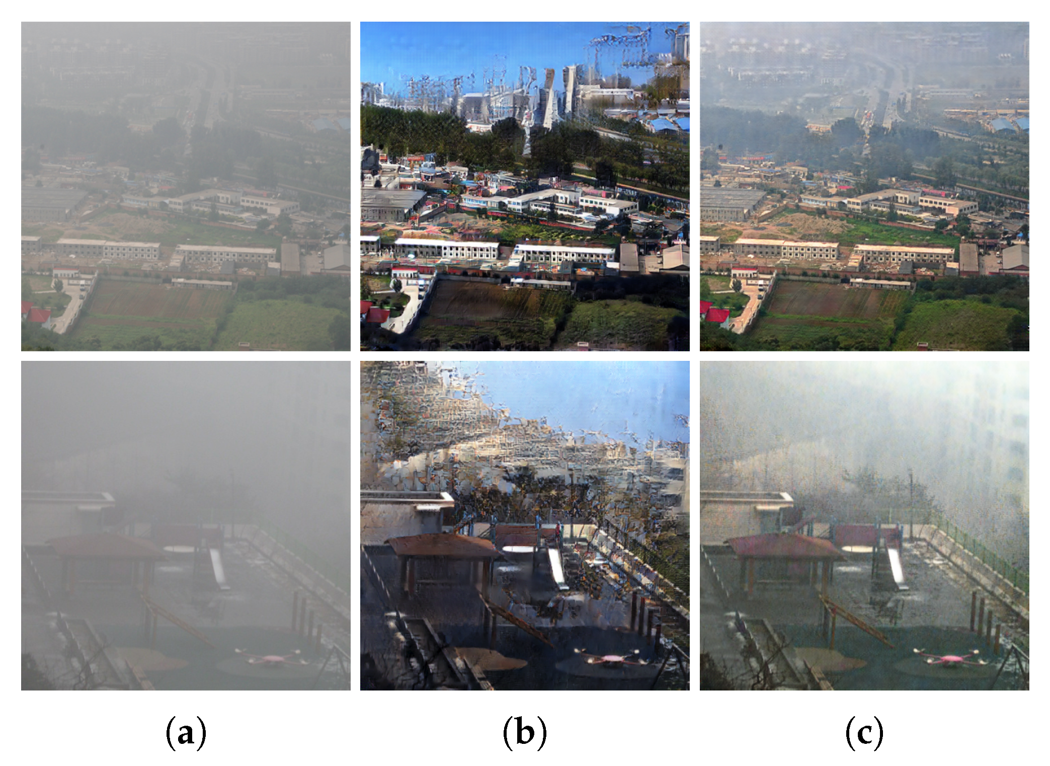
The results are reported in

Table 5. Indicators e and $\overline{r}$ from [15], the proposed HArD metric and the indicators HArD + e and HArD + $\overline{r}$ calculated on the LIVE test set. ↑ indicates that a higher value is better, ↓ indicates that a lower value is better.

	Cycle-Dehaze [7]	Pix2Pix [34]	CurL-Defog
HArD (↓)	2.535	0.3786	1.374
e (↑)	32.70	25.74	28.41
HArD+e (↑)	30.58	25.73	26.76
$\overline{r}$ (↑)	3.290	2.135	2.636
HArD+$\overline{r}$ (↑)	2.998	2.131	2.537

, and some examples are shown in Figure 8. As we can see from Figure 8, CurL-Defog often produces more realistic results compared to Cycle–Dehaze [7], with almost no artifacts inserted into the defogged image. On the other hand, Cycle–Dehaze produces slightly more contrasted and sharper results, at the cost of a greater introduction of unwanted objects in the scene. At the same time, the amount of details produced by CurL-Defog, especially on very foggy regions, was better than pix2pix. The HArD values in Table 5 support these observations. As stated before, the indicators e and $\overline{r}$ are affected by the insertion of artifacts; therefore, they cannot be considered in isolation, especially when they are used to evaluate unpaired defogging approaches. The proposed indicators HArD + e and HArD + $\overline{r}$ should give a more valid indication of the quality of the defogging procedure since the effect of artifacts was discounted. We observe that, excluding the artifact regions, the values of e and $\overline{r}$ were reduced (except for pix2pix, which was almost artifact-free). The reduction was more marked for Cycle–Dehaze than for CurL-Defog; in particular, for the value of $\overline{r}$, the reductions were 9.7% and 3.9%, respectively. However, the adjusted metrics still showed that the contrast improvement was larger for Cycle–Dehaze. The performance of CurL-Defog was in the middle of this range, enhancing the contrast better than the pix2pix model while producing a low number of artifacts.

Overall, as discussed in Section 4, these results show that a single defogging metric that takes into account every aspect is still lacking; thus, using complementary metrics that focus on different aspects is the best choice to properly evaluate and compare different approaches. When ground-truth data are available, reference-based metrics remain the most obvious choice, but unfortunately in challenging cases with real severe fog, reliable reference images are very difficult to obtain (if the fog is not artificial, the two images need to be taken at different times (maybe one or more days later) and to avoid unwanted changes at pixel level: (i) the camera must be firmly fixed to avoid any image misalignment; (ii) the lighting conditions must be similar (e.g., shadows); (iii) moving objects should be absent (clouds, cars, pedestrians, tree leaves, etc.); and (iv) wind (even light wind) should be avoided, as it could bend trees or move other objects).

5.5. Experiments on Severe Fog

To further assess the quality of the proposed CurL-Defog approach in the presence of severe fog, we tested our model using the Dense-Haze dataset [12], which is composed of 55 images in which fog is artificially inserted with fog-machines in controlled conditions. This makes a direct comparison (in terms of classical PSNR and SSIM) with clear images of the same scene possible. We also used CIEDE2000 [43] to assess the fidelity of color appearance. CIEDE2000 measures the color difference between two images and generates smaller values for better color preservation. The level of the fog of the images is significant, and the visibility is almost zero in all the photographs. We compared our method with several state-of-the-art learning-based defogging techniques [2,3,7,34]. The datasets used in this experiment were as follows:

• Synthetic paired dataset (training): The Outdoor Training Set (OTS), included in the RESIDE dataset [9], which was used to train pix2pix and the paired part of CurL-Defog;
• Real unpaired dataset (training): The O-Haze dataset [44], which is composed of 45 high-resolution pairs of fog and real images. The fog is inserted with fog machines and it is very similar to real fog. However, the level of fog is much less than in the Dense-Haze dataset. We randomly cropped each of the 45 images 45 times, producing an unpaired dataset of 2025 images. We used this training set during the training of Cycle-Dehaze and CurL-Defog;
• Test dataset: The Dense-Haze dataset (55 images with severe fog) [12].

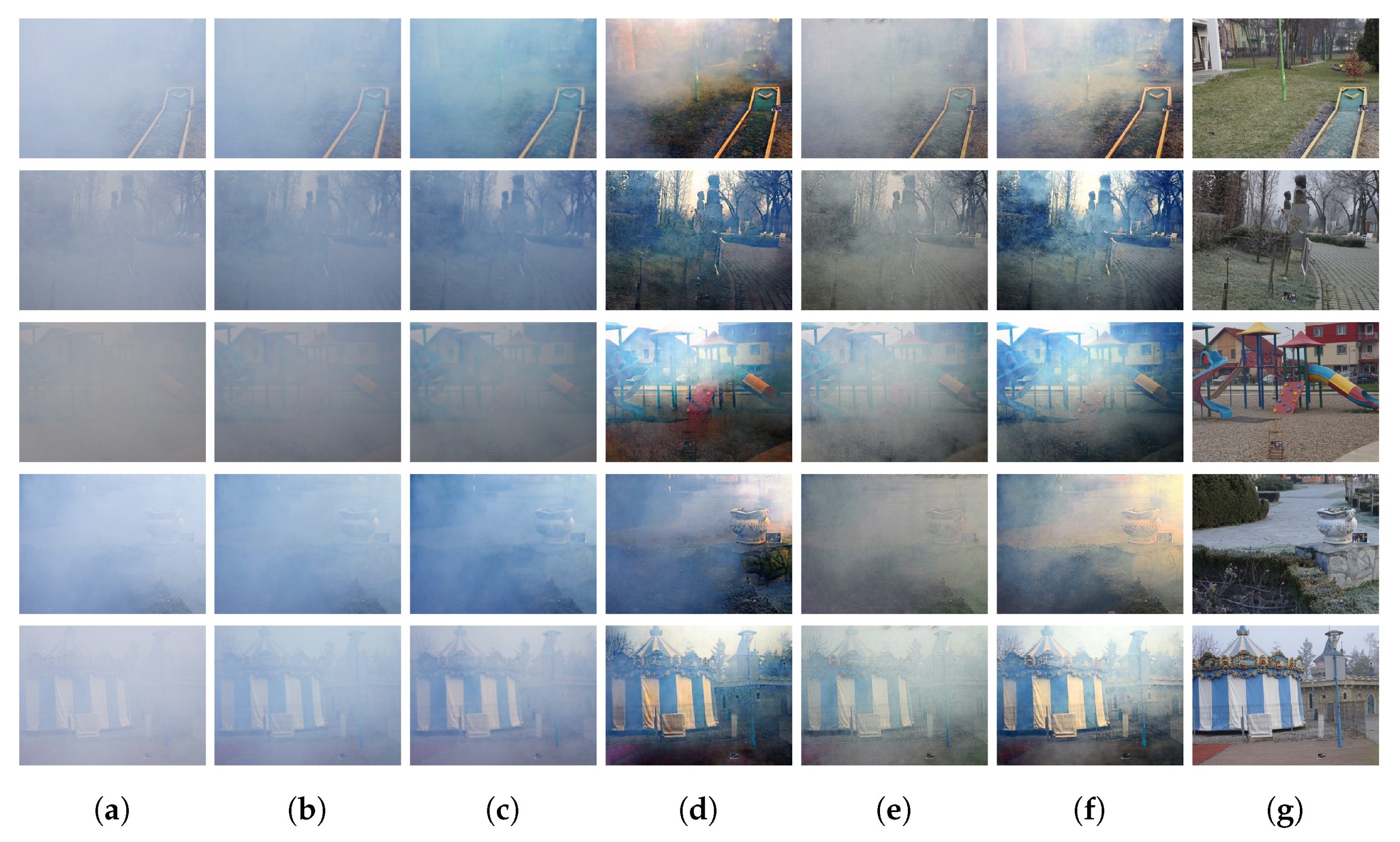
The results are reported in

Table 6. Average SSIM, PSNR, and CIEDE2000 scores of the dehazing on the Dense-Haze dataset.

	PSNR (↑)	SSIM (↑)	CIEDE2000 (↓)
MSCNN [3]	12.52	0.369	24.69
DehazeNet [2]	11.36	0.374	26.88
CycleDehaze [7]	10.54	0.261	25.12
Pix2Pix [34]	10.55	0.311	25.22
CurL-Defog	12.24	0.469	24.86

. Note that our method was not trained with images of the Dense-Haze dataset, nor with images with a comparable high level of fog. The results in Table 6 demonstrate the effectiveness of CurL-Defog: our approach showed similar performance on the PSNR and CIEDE2000 metrics with regard to the best baseline, but greatly outperformed all the methods on the SSIM metric. This means that the original colors were correctly maintained after the defogging, and both absolute and perception errors were minimized compared to the direct competitors pix2pix [34] and Cycle–Dehaze [26]. Some examples of the result on the Dense-Haze dataset are shown in Figure 9. As we can see from the figure, our method produced better defogged results in comparison with the other baselines and did not insert artifacts even in this extreme scenario. Pix2pix yielded very appealing results that were similar to those generated by CurL-Defog. However, the CIEDE2000 metric showed a slightly better color preservation for CurL-Defog (Table 6, third row). This can be partially appreciated by comparing the images in columns (d), (e) and (g) in Figure 9.

5.6. Inference Time Calculation

In order to assess the practical applicability of CurL-Defog, we calculated the inference time of the proposed approach using a CPU and GPU. A possible application for CurL-Defog could be self-driving cars, where it could be used to enhance the images acquired by the cameras under poor weather conditions. We argue that in future cars, where Advanced Driver Assistance Systems (ADAS) will be pervasive, the presence of a GPU (or some dedicated hardware for image and signal processing) will be standard. We tested CurL-Defog using $512\times 512$ and high-resolution $1024\times 1024$ images. The CPU used was an Intel Xeon E5-2650; the GPU used was an NVIDIA GeForce GTX 1080Ti. The inference times are reported in

Table 7. Average inference time and frames per second of CurL-Defog. All the tests were performed using 100 images from the LIVE image defogging test set [42].

Device	CPU	GPU
Image Size	$512\times 512$	$512\times 512$	$1024\times 1024$
Mean inference time (1 image)	1.8821 s	0.0248 s	0.0337 s
FPS	∼0.5	∼40	∼30

. The results showed that Curl-Defog can run in real-time on a mid-range GPU.

6. Conclusions

In this paper, we proposed CurL-Defog, a defogging approach based on curriculum learning and generative adversarial networks, with the aim of reducing the number of artifacts in the output images. CurL-Defog exploits both paired and unpaired data to effectively defog images, even in the presence of severe fog. Paired synthetic images force the model not to introduce artifacts in the results, while using real images ensures a satisfactory defogging of real data. Moreover, to automatically localize and numerically estimate the amount of artifacts produced after the defogging, we proposed HArD, a new, referenceless artifact detection technique. We also combined HArD with pre-existent defogging metrics, producing the indicators HArD + e and HArD + $\overline{r}$. The experiments on CurL-Defog demonstrate the quality of our approach, with the method matching or improving on state-of-the-art methods on both synthetic and real data. Our study confirmed that the information provided by paired data is useful to guide the model towards regions of the parameter space that minimize the insertion of artifacts, especially in the case of severe fog. We also tested our model in extreme conditions using severely fogged images, and even in this case, CurL-Defog proved to be reliable and in line with the current state-of-the-art approaches.

Some aspects that we did not consider in this work are foggy night photographs and videos. Night photos are complex to handle due to the low ambient illumination and light reflections. On the other hand, videos could be exploited to detect and remove artifacts, since temporal coherence can be exploited to discriminate between real objects (appearing at close locations across consecutive frames) and artifacts whose generation is more random. Moreover, we would like to investigate the advantages of replacing the gradient operator in HArD with alternative operators that better correlate with the human visual system [38,39].

References

1. Li, Y.; You, S.; Brown, M.S.; Tan, R.T. Haze Visibility Enhancement: A Survey and Quantitative Benchmarking. Comput. Vis. Image Underst. 2017, 165, 1–16. [Google Scholar] [CrossRef] [Green Version]
2. Cai, B.; Xu, X.; Jia, K.; Qing, C.; Tao, D. Dehazenet: An End-to-End System for Single Image Haze Removal. IEEE Trans. Image Process. 2016, 25, 5187–5198. [Google Scholar] [CrossRef] [PubMed] [Green Version]
3. Ren, W.; Liu, S.; Zhang, H.; Pan, J.; Cao, X.; Yang, M.H. Single Image Dehazing via Multi-Scale Convolutional Neural Networks. In European Conference on Computer Vision; Springer: Berlin, Germany, 2016; pp. 154–169. [Google Scholar]
4. Li, B.; Peng, X.; Wang, Z.; Xu, J.; Feng, D. Aod-net: All-in-One Dehazing Network. In Proceedings of the IEEE International Conference on Computer Vision, Venice, Italy, 27–29 October 2017; pp. 4770–4778. [Google Scholar]
5. Pang, Y.; Xie, J.; Li, X. Visual Haze Removal by a Unified Generative Adversarial Network. IEEE Trans. Circuits Syst. Video Technol. 2018, 29, 3211–3221. [Google Scholar] [CrossRef]
6. Li, R.; Pan, J.; Li, Z.; Tang, J. Single Image Dehazing via Conditional Generative Adversarial Network. In Proceedings of the 2018 IEEE/CVF Conference on Computer Vision and Pattern Recognition, Salt Lake City, UT, USA, 18–22 June 2018; pp. 8202–8211. [Google Scholar]
7. Engin, D.; Genç, A.; Ekenel, H.K. Cycle-Dehaze: Enhanced CycleGAN for Single Image Dehazing. In Proceedings of the IEEE Conference on Computer Vision and Pattern Recognition (CVPR) Workshops, Salt Lake City, UT, USA, 18–22 June 2018. [Google Scholar]
8. Liu, W.; Hou, X.; Duan, J.; Qiu, G. End-to-End Single Image Fog Removal Using Enhanced Cycle Consistent Adversarial Networks. arXiv 2019. Available online: https://www.researchgate.net/publication/330870807_End-to-End_Single_Image_Fog_Removal_using_Enhanced_Cycle_Consistent_Adversarial_Networks (accessed on 27 April 2020).
9. Li, B.; Ren, W.; Fu, D.; Tao, D.; Feng, D.; Zeng, W.; Wang, Z. Benchmarking Single-Image Dehazing and Beyond. IEEE Trans. Image Process. 2019, 28, 492–505. [Google Scholar] [CrossRef] [PubMed] [Green Version]
10. Tarel, J.P.; Hautiere, N.; Caraffa, L.; Cord, A.; Halmaoui, H.; Gruyer, D. Vision Enhancement in Homogeneous and Heterogeneous Fog. IEEE Intell. Trans. Syst. Mag. 2012, 4, 6–20. [Google Scholar] [CrossRef] [Green Version]
11. Cosmin, A.; Codruta, O.; Ancuti, C.D.V. D-Hazy: A Dataset to Evaluate Quantitatively Dehazing Algorithms. In Proceedings of the IEEE International Conference on Image Processing (ICIP), Phoenix, AZ, USA, 25–28 September 2016. [Google Scholar]
12. Ancuti, C.O.; Ancuti, C.; Sbert, M.; Timofte, R. Dense Haze: A Benchmark for Image Dehazing with Dense-Haze and Haze-Free Images. In Proceedings of the IEEE International Conference on Image Processing (ICIP), Taipei, Taiwan, 22–25 September 2019. [Google Scholar]
13. Bengio, Y.; Louradour, J.; Collobert, R.; Weston, J. Curriculum Learning. In Proceedings of the 26th International Conference on Machine Learning, Montreal, QC, Canada, 14–18 June 2009; pp. 41–48. [Google Scholar]
14. Hacohen, G.; Weinshall, D. On the power of curriculum learning in training deep networks. arXiv 2019, arXiv:1904.03626. [Google Scholar]
15. Hautiere, N.; Tarel, J.P.; Aubert, D.; Dumont, E. Blind Contrast Enhancement Assessment by Gradient Ratioing at Visible Edges. Image Anal. Stereol. 2011, 27, 87–95. [Google Scholar] [CrossRef]
16. Graffieti, G.; Maltoni, D. Towards Artifacts-Free Image Defogging. In Proceedings of the 25th International Conference on Pattern Recognition (ICPR), Milano, Italy, 15 January 2021; pp. 5060–5067. [Google Scholar]
17. Koschmieder, H. Theorie der horizontalen Sichtweite. Beitrage Physik Freien Atmos. 1924, 12, 33–53. [Google Scholar]
18. McCartney, E.J. Optics of the Atmosphere: Scattering by Molecules and Particles; John Wiley and Sons, Inc.: New York, NY, USA, 1976; 421p. [Google Scholar]
19. Narasimhan, S.G.; Nayar, S.K. Interactive (de) Weathering of an Image Using Physical Models. In Proceedings of the IEEE Workshop on Color and Photometric Methods in Computer Vision, Nice, France, 13–16 October 2003; Volume 6, p. 1. [Google Scholar]
20. Fattal, R. Single Image Dehazing. ACM Trans. Graph. (TOG) 2008, 27, 1–9. [Google Scholar] [CrossRef]
21. He, K.; Sun, J.; Tang, X. Single Image Haze Removal using Dark Channel Prior. IEEE Trans. Pattern Anal. Mach. Intell. 2010, 33, 2341–2353. [Google Scholar] [PubMed]
22. Tarel, J.P.; Hautiere, N. Fast Visibility Restoration from a Single Color or Gray Level Image. In Proceedings of the 2009 IEEE 12th International Conference on Computer Vision, Kyoto, Japan, 29 September–2 October 2009; pp. 2201–2208. [Google Scholar]
23. Zhu, Q.; Mai, J.; Shao, L. A Fast Single Image Haze Removal Algorithm Using Color Attenuation Prior. IEEE Trans. Image Process. 2015, 24, 3522–3533. [Google Scholar] [PubMed] [Green Version]
24. Berman, D.; Avidan, S. Non-Local Image Dehazing. In Proceedings of the IEEE Conference on Computer Vision and Pattern Recognition, Las Vegas, NV, USA, 27–30 June 2016; pp. 1674–1682. [Google Scholar]
25. Goodfellow, I.J.; Pouget-Abadie, J.; Mirza, M.; Xu, B.; Warde-Farley, D.; Ozair, S.; Courville, A.; Bengio, Y. Generative Adversarial Nets. In Proceedings of the 27th International Conference on Neural Information Processing Systems; MIT Press: Cambridge, MA, USA, 2014; Volume 2, pp. 2672–2680. [Google Scholar]
26. Zhu, J.Y.; Park, T.; Isola, P.; Efros, A.A. Unpaired Image-to-Image Translation using Cycle-Consistent Adversarial Networks. In Proceedings of the 2017 IEEE International Conference on Computer Vision, Venice, Italy, 22–29 October 2017. [Google Scholar]
27. Johnson, J.; Alahi, A.; Fei-Fei, L. Perceptual Losses for Real-Time Style Transfer and Super-Resolution. In European Conference on Computer Vision ECCV; Springer: Cham, Switzerland, 2016. [Google Scholar]
28. Simonyan, K.; Zisserman, A. Very Deep Convolutional Networks for Large-Scale Image Recognition. arXiv 2014, arXiv:1409.1556. [Google Scholar]
29. Sakaridis, C.; Dai, D.; Hecker, S.; Van Gool, L. Model Adaptation with Synthetic and Real Data for Semantic Dense Foggy Scene Understanding. In European Conference on Computer Vision (ECCV); Springer: Cham, Switzerland, 2018; pp. 707–724. [Google Scholar]
30. Dai, D.; Sakaridis, C.; Hecker, S.; Van Gool, L. Curriculum Model Adaptation with Synthetic and Real Data for Semantic Foggy Scene Understanding. Int. J. Comput. Vis. 2020, 128, 1182–1204. [Google Scholar] [CrossRef] [Green Version]
31. Wang, Z.; Bovik, A.C.; Sheikh, H.R.; Simoncelli, E.P. Image Quality Assessment: From Error Visibility to Structural Similarity. IEEE Trans. Image Process. 2004, 13, 600–612. [Google Scholar] [CrossRef] [PubMed] [Green Version]
32. CIE. International Lighting Vocabulary. CIE 17.4-1987. 1987. Available online: https://cie.co.at/publications/international-lighting-vocabulary (accessed on 27 April 2021).
33. Choi, L.K.; You, J.; Bovik, A.C. Referenceless Prediction of Perceptual Fog Density and Perceptual Image Defogging. IEEE Trans. Image Process. 2015, 24, 3888–3901. [Google Scholar] [CrossRef] [PubMed]
34. Isola, P.; Zhu, J.Y.; Zhou, T.; Efros, A.A. Image-to-Image Translation with Conditional Adversarial Networks. arXiv 2016, arXiv:1611.07004. [Google Scholar]
35. Ulyanov, D.; Vedaldi, A.; Lempitsky, V.S. Instance Normalization: The Missing Ingredient for Fast Stylization. arXiv 2016, arXiv:1607.08022. [Google Scholar]
36. He, K.; Zhang, X.; Ren, S.; Sun, J. Deep Residual Learning for Image Recognition. In Proceedings of the 2016 IEEE Conference on Computer Vision and Pattern Recognition (CVPR), Las Vegas, NA, USA, 27–30 June 2016; pp. 770–778. [Google Scholar]
37. Ledig, C.; Theis, L.; Huszár, F.; Caballero, J.; Cunningham, A.; Acosta, A.; Aitken, A.; Tejani, A.; Totz, J.; Wang, Z. Photo-Realistic Single Image Super-Resolution using a Generative Adversarial Network. In Proceedings of the IEEE Conference on Computer Vision and Pattern Recognition, Honolulu, HI, USA, 21–26 June 2017; pp. 4681–4690. [Google Scholar]
38. Michelson, A.A. Studies in Optics; The University of Chicago Press: Chicago, IL, USA, 1927. [Google Scholar]
39. Jourlin, M.; Pinoli, J.C.; Zeboudj, R. Contrast definition and contour detection for logarithmic images. J. Microsc. 1989, 156, 33–40. [Google Scholar] [CrossRef] [PubMed]
40. Shrivastava, A.; Pfister, T.; Tuzel, O.; Susskind, J.; Wang, W.; Webb, R. Learning from Simulated and Unsupervised Images through Adversarial Training. In Proceedings of the IEEE Conference on Computer Vision and Pattern Recognition, Honolulu, HI, USA, 21–26 June 2017; pp. 2107–2116. [Google Scholar]
41. Wang, Z.; Simoncelli, E.P.; Bovik, A.C. Multiscale Structural Similarity for Image Quality Assessment. In Proceedings of the Thrity-Seventh Asilomar Conference on Signals, Systems Computers, Pacific Grove, CA, USA, 9–12 November 2003; Volume 2, pp. 1398–1402. [Google Scholar]
42. Choi, L.K.; You, J.; Bovik, A.C. LIVE Image Defogging Database. Available online: http://live.ece.utexas.edu/research/fog/fade_defade.html (accessed on 30 May 2019).
43. Sharma, G.; Wu, W.; Dalal, E.N. The CIEDE2000 color-difference formula: Implementation notes, supplementary test data, and mathematical observations. Color Res. Appl. 2005, 30, 21–30. [Google Scholar] [CrossRef]
44. Ancuti, C.O.; Ancuti, C.; Timofte, R.; De Vleeschouwer, C. O-HAZE: A Dehazing Benchmark with Real Hazy and Haze-Free Outdoor Images. In Proceedings of the IEEE Conference on Computer Vision and Pattern Recognition Workshops, Salt Lake City, UT, USA, 18–22 June 2018; pp. 754–762. [Google Scholar]
Figure 1. (a) Real severely fogged images; (b) defogging with a state-of-the-art unpaired approach [7]. Note the clear artifacts in the sky; (c) the results produced by the proposed CurL-Defog, denoting a good compromise between image enhancement and fidelity to the original scene. Images are better viewed if enlarged on a computer monitor.
Atmosphere 12 00577 g001
Figure 2. CurL-Defog architecture. (a) During the paired training, two separate pix2pix models are used: one for defogging and one for fogging images. (b) During the unpaired training, the two generators are used in combination to enforce the cycle consistency loss and the cycle perceptual loss; to keep the notation simple, the discriminators are depicted as rectangles, and in (b), only the defogging cycle is displayed, since the foggy cycle (starting from the clear image) is symmetrical and can be easily derived. For each training epoch, the model behaves as in (a) for a subset of the training iterations, and as in (b) for the rest of the iterations.
Atmosphere 12 00577 g002
Figure 3. Overall sequence of steps in HArD metric calculation. (a) Input images: the top row is the real fogged image, the second row is the same image defogged by a pure unpaired approach [26]. (b) Gradient computation by the Prewitt operator. (c) Smoothing with a Gaussian filter and scaling in the interval [0,1]. (d) Saturation of the maps through the hyperbolic tangent. (e) Difference between the two maps in (d). (f) The regions where the metrics detected the presence of artifacts superimposed over the defogged image. Images are better viewed if enlarged on a computer monitor.
Atmosphere 12 00577 g003
Figure 4. Some examples of the region detected by the HArD metric using real and synthetic images with different levels of inserted artifacts. The first two lines refer to real images with a heavy introduction of artifacts. The third row shows a real image with a very low insertion of artifacts. The last row includes a synthetic foggy image and the corresponding ground truth. (a) Foggy images (b) Defogged images (c) The regions where the HArD metrics detected the presence of artifacts, and (d) the regions of detected artifacts superimposed on the defogged image. Images are better viewed if enlarged on a computer monitor.
Atmosphere 12 00577 g004
Figure 5. An example showing how the indicators e and r ¯ proposed by Hautiére et al. [15] could be deceived by the presence of artifacts. (a) Foggy image and the corresponding defogging with a massive presence of artifacts, (b) the gradients of the two images and the corresponding ratio (third row). Note that where artifacts are present, the ratio is very high. Bright red denotes a ratio larger than 10. (c) Visible edges in the two images and the visible edges only present in the defogging. Note that the majority of visible edges in the defogged image are in regions where artifacts are clearly present. Images are better viewed if enlarged on a computer monitor.
Atmosphere 12 00577 g005
Figure 6. Benefits of HArD + e and HArD + r ¯ over the simple indicators e and r ¯ . (a) Real foggy images, (b) defogged images with various level of artifacts, (c) the binarized mask obtained from the HArD metric, (d) the visible edges in the defogged image. Note the high number of edges in regions where artifacts are present. (e) Visible edges used to compute HArD + e and HArD + r ¯ ; note that edges belonging to artifacts are not considered. (f) The ratio of the gradients between the defogged and the foggy images. Note the high value in regions where artifacts are massively present (bright red indicates a ratio greater than 10). (g) The ratio used to calculate HArD+ r ¯ . Note the near-absence of regions with a saturated gradient. Images are better viewed if enlarged on a computer monitor.
Atmosphere 12 00577 g006
Figure 7. Qualitative comparison of defogging on two sample images extracted from the HSTS synthetic test set [9]. (a) Foggy images, (b) defogging by CAP [23], (c) defogging by DehazeNet [2], (d) defogging by AOD-Net [4], (e) pix2pix [34], (f) CurL-Defog (our method), and (g) ground-truth images. Images are better viewed if enlarged on a computer monitor.
Atmosphere 12 00577 g007
Figure 8. Qualitative comparison of defogging on real images with severe fog. (a) Foggy images, (b) unpaired approach [7] (note the heavy insertion of artifacts), (c) paired approach [34], (d) CurL-Defog. Images are better viewed if enlarged on a computer monitor.
Atmosphere 12 00577 g008
Figure 9. Qualitative comparison of defogging on the Denze-Haze dataset [12]. (a) Foggy images, (b) defogging by [2], (c) defogging by [3], (d) pix2pix [34], (e) Cycle–Dehaze [7], (f) CurL-Defog (our approach), (g) ground-truth image. Images are better viewed if enlarged on a computer monitor.
Atmosphere 12 00577 g009